Research Division
Federal Reserve Bank of St. Louis
Working Paper Series
Inter-temporal Differences in the Income Elasticity of Demand
for Lottery Tickets
Thomas A. Garrett
and
Cletus C. Coughlin
Working Paper 2007-042C http://research.stlouisfed.org/wp/2007/2007-042.pdf October 2007 Revised August 2008FEDERAL RESERVE BANK OF ST. LOUIS Research Division
P.O. Box 442 St. Louis, MO 63166
______________________________________________________________________________________ The views expressed are those of the individual authors and do not necessarily reflect official positions of the Federal Reserve Bank of St. Louis, the Federal Reserve System, or the Board of Governors.
Federal Reserve Bank of St. Louis Working Papers are preliminary materials circulated to stimulate discussion and critical comment. References in publications to Federal Reserve Bank of St. Louis Working Papers (other than an acknowledgment that the writer has had access to unpublished material) should be cleared with the author or authors.
Inter-temporal Differences in the Income Elasticity of Demand for Lottery Tickets
Thomas A. Garrett
Federal Reserve Bank of St. Louis P.O. Box 442
St. Louis, Missouri 63166 (314) 444-8601 garrett@stls.frb.org
Cletus C. Coughlin
Federal Reserve Bank of St. Louis P.O. Box 442
St. Louis, Missouri 63166 (314) 444-8585 coughlin@stls.frb.org
Abstract
We estimate annual income elasticities of demand for lottery tickets using county-level panel data for three states and find that the income elasticity of demand (and thus the tax burden) for lottery tickets has changed over time. This is due to changes in a state’s lottery game portfolio and the growth in consumer income more so than competition from alternative gambling opportunities. Trends in the income elasticity for instant and online lottery games appear to be different. Our results raise doubts about the long-term growth potential of lottery revenue and have policy implications for state governments and those concerned about regressivity.
JEL Codes: H71, H22
Keywords: state lotteries, tax incidence, regressivity, income elasticity ________________
We thank the Florida Lottery, the Iowa Lottery, and the West Virginia Lottery for providing lottery sales data. The views expressed are those of the authors and do not necessarily reflect the views of the Federal Reserve Bank of St. Louis or the Federal Reserve System. Lesli Ott provided research assistance.
Inter-temporal Differences in the Income Elasticity of Demand for Lottery Tickets
Introduction
Beginning with New Hampshire in 1964, forty-two states and the District of Columbia have legalized state-sponsored lotteries. Lottery sales in the United States topped $48 billion in fiscal year 2006 (roughly $160 per capita), of which state governments retained nearly $17 billion (about 1 percent of total state government revenue) for spending on education, infrastructure, and other social programs. The preceding sales and tax revenues suggest an average tax rate of 35 percent, an average rate much higher than that of other state excise taxes (Clotfelter and Cook, 1987). The growth in lottery sales over the past several decades is not only a result of more state lotteries, but by an ever evolving product line that is designed to attract and retain customers through higher jackpots, some reaching several hundred million dollars.
The growth of the lottery industry has sparked much research. Numerous studies, including Filer et al. (1988), Davis et al. (1992), and Alm et al. (1993), have explored the determinants of a state’s decision to adopt a lottery.1 The optimal design of lottery games in terms of maximizing sales was studied by Quiggin (1991), Cook and Clotfelter (1993), and Garrett and Sobel (1999). Whether lottery ticket purchases are substit
complements for other consumer goods has been explored by Borg et al. (1993) and Kearney (2005). The revenue impact of cross-border lottery shopping has been studied by Garrett and Marsh (2002) and Tosun and Skidmore (2004). Similarly, Brown and Rork (2005) examined the strategic interaction between state lotteries using a model of tax competition. Finally, because states earmark net lottery revenues for programs such
utes or
1
as education, several studies have explored whether lottery revenues increase spending on the target program (Borg and Mason, 1990; Spindler, 1995; Novarro, 2005).
The issue that has received the greatest attention is the tax incidence of lottery ticket expenditures for different income groups (Clotfelter and Cook, 1987, 1989; Scott and Garen, 1994; Hansen, 1995; Farrell et al. 1999; Price and Novak, 1999; and Forrest et al., 2000).2 Studies have used data of various levels of aggregation, such as individual survey data as well as aggregate data for zip codes, cities, counties, and states. The majority of research has shown that state lotteries can be characterized as regressive taxation, implying a decreasing tax burden in relative terms as incomes rises.3 Not surprisingly, this tax regressivity is raised as an objection to state lotteries, especially in light of the revenue maximization objective of state lottery agencies.
In most lottery demand studies a single income elasticity of demand is estimated from the sample of data, thus providing a static look at the tax incidence of lottery tickets. The results from previous research allow a comparison of a single income elasticity estimate from one study (state, county, city, or zip code at a point in time) with another study (another state, county, city, or zip code at a point in time), but little evidence exists on how the income elasticity of demand for a specific state’s lottery product has changed over time. As discussed in the next section, rising consumer income, the introduction of new games, and other changes in the gambling landscape suggest that the tax incidence of lottery expenditures has not remained constant over time.
This paper provides evidence on the dynamic nature of the income elasticity of demand for lottery tickets. Using a panel of annual county-level data for three states that
2
This is not a complete list of all lottery demand studies. See the above studies for additional research.
3
For example, Miyazaki et al. (1998) found 19 of 27 cases in which the specific lottery was regressive. Cases of proportionality and progressivity were also found.
have had a lottery for seventeen or more years, we estimate annual income elasticities of demand for each state. This provides a sufficient time series to track how the income elasticity of demand for lottery tickets, and thus the lottery tax burden, in each state has changed over the past several years.4 We link the trends in the income elasticity of demand over time to possible business cycle effects, the introduction of new lottery products, and changes in consumer income. Our framework also allows us to explore whether growing competition for lottery products from casino gambling and neighboring state lottery games has changed the income elasticity of demand for lottery tickets.
Our results shed new light on the dynamic nature of lottery tax burdens and suggest that income elasticities estimated from a single year of data, as has been done in much of the past research, may accurately reflect the income elasticity of demand only for a specific year. The degree of lottery regressivity or progressivity is time dependent. Our annual estimates also provide a picture of the long term revenue prospects of the state lotteries studied here, an important issue for all lottery states and programs funded by lottery revenue. Our evidence suggests that the long-term revenue prospects of state lotteries are unfavorable compared to other sources of state tax revenue.
Income Elasticities over Time: Theory
There are several reasons to expect the income elasticity of demand for lottery tickets to change over time. The most general is that consumer income has generally increased over time. A consistent empirical finding is that as income rises, individuals
4
Changing income elasticities provide evidence on the changing tax regressivity or progressivity of the lottery. An income elasticity exceeding one indicates that the lottery tax is progressive, an income elasticity equal to one indicates the lottery tax is proportional, and an income elasticity less than one (including negative values) indicates that the lottery tax is regressive. If the income elasticity is less than one and is declining (increasing) over time, then the lottery tax is becoming more (less) regressive.
spend a smaller share of their budgets on lottery tickets (i.e., the income elasticity is less than one). Thus, as incomes tend to rise over time, the income elasticity of demand for lottery tickets should decline.5
In addition to changes in income, the competitive environment in which state lotteries operate has changed over time. For example, relative to the mid 1980s, today’s environment includes different advertising campaigns, new lottery games, more gaming alternatives (e.g., casino gaming and lotteries in neighboring states), and increased information about games. Attitudes about gaming may have also changed. In theory, however, how a specific change may affect the income elasticity of demand is often uncertain. The reason for this uncertainty is that a specific change must affect spending (in percentage terms) by individuals with different incomes differentially.6
Consider how advertising expenditures might affect the income elasticity of lottery demand. Increased lottery-related advertising should lead to increased spending on lottery tickets; however, the effect of increased advertising expenditures on the income elasticity of lottery demand depends on how the spending patterns of individuals change. The income elasticity could increase, decrease, or remain unchanged.7 Many advertising campaigns are targeted to certain groups, so specific advertising campaigns
5
This reasoning applies to many goods. For example, decades ago foreign travel was a luxury (i.e., the income elasticity of demand for foreign travel exceeded one). Today, with higher incomes, foreign travel has become much less of a luxury for most and a necessity for some.
6
Because our empirical analysis uses counties rather than individuals as our unit of observation, the specific change must cause different percentage changes in lottery spending across counties. Such a difference does not invalidate the argument.
7
To illustrate, assume two individuals whose spending on lottery tickets and incomes are as follows: player #1 - $100 spending with $10,000 income and player #2 - $150 spending with $20,000 income. In this case, the income elasticity is 0.5. Assume an advertising campaign that causes both players to spend an
additional ten percent on lottery tickets. With player #1 spending $110 and player #2 spending $165, the income elasticity remains at 0.5. If, however, the percentage change in spending differs between the two players, then the income elasticity will change. If spending by player #1 increased from $100 to $105 and spending by player #2 increased from $150 to $165, then the income elasticity would be greater than 0.5. On the other hand, if spending by player #1 increased from $100 to $115 and spending by player #2 increased from $150 to $165, then the income elasticity would be less than 0.5.
are undertaken with an expectation of affecting groups differentially.8 An effective promotional campaign targeting low-income players should tend to reduce the income elasticity of lottery demand, while an effective promotional campaign targeting high-income players should tend to increase the high-income elasticity of lottery demand. A final observation is that an advertising campaign is often tied to the introduction of a new game, which itself might be targeted to appeal to a certain audience.
New lottery game introduction within a state may also result in changing income elasticities of demand over time. State lotteries have attempted to maintain player excitement about the lottery by adding instant and online games that offer higher jackpots. For example, many states participate in multi-state online lottery games that generate much larger jackpots than could be offered from relying on lottery sales in a single state. The odds of winning the jackpot in the multi-state game PowerBall have been decreased several times to generate jackpots totaling hundreds of millions of dollars. In addition, starting in the 1990s many states began to offer $2, $5, or even $10 and $20 instant lottery games that offer much higher jackpots ($1 or $2 million) and payout rates (above 60 percent) than the traditional $1 instant game (payout rates averaging 50 percent).9 Research by Mikesell (1989) and Oster (2004) suggests that large jackpot online lottery games may attract a wealthier player than lower jackpot instant games and thus may increase the income elasticity of demand.10
8
The Massachusetts lottery has placed Spanish-language ads in Hispanic newspapers, radio stations, and
websites. See “Marketing is the Ticket for Massachusetts State Lottery.” Boston Globe, April 2, 2008, A.1.
9
Contacts at state lottery agencies confirm that higher priced instant games have, on average, higher payout rates than traditional $1 instant lottery games.
10
Because we have aggregated game data (online and instant), it is difficult for us to examine how changes in payout rates affect the distribution of lottery players for two reasons. First, payout rates are only changed for online pari-mutuel games on an infrequent basis, usually by worsening the odds of winning by adding more combinations. Second, the expected return to players can change drawing to drawing for pari-mutuel online games when roll-overs occur and the jackpot grows. These high frequency events cannot be
Furthermore, the magnitude of the change in the income elasticity of lottery demand likely differs for instant lottery games and online lottery games. Instant lottery games typically offer prizes ranging from about $100,000 to $250,000, with some offering a top prize of $1 or $2 million.11 Although these amounts have increased over time, the top prize amounts for online lotto games have increased much more – top prizes in the 1980s and early 1990s were typically several million dollars, whereas today top prizes reach hundreds of millions of dollars.
Income elasticities of lottery demand may also change over time due to the introduction of lotteries in neighboring states and by the introduction of casino gaming that has occurred in many states since the early to mid 1990s. The start of a lottery in a neighboring state is likely to have larger effects on counties that border the state than on counties that do not border the state. Later, we explore empirically how the income elasticity of demand for lottery tickets has changed as a result of lottery game
introduction in a border state as well as the introduction of casino gambling. The key to any change in the income elasticity of lottery demand is whether the specific border counties are affected differently. If lottery spending in each border county is affected identically in percentage terms from the introduction of a lottery in a border state, then the income elasticity of lottery demand will be unchanged for both the border counties and the entire state. However, it is possible that the border counties and the casino counties will each be affected differently relative to other counties, but exactly how is uncertain. Moreover, even if the income elasticity of the border counties and casino
captured with our annual level data. However, the effect that the introduction of an online game that has different payout rates over time (e.g., PowerBall) has on the distribution of lottery players can be captured by our annual income elasticity estimates.
11
counties change, it is uncertain how the income elasticity for the entire state will change.12
In sum, changes in the income elasticity of demand for lottery tickets likely depends upon various factors, such as income growth, lottery advertising, the
introduction of new games, whether a neighboring state has a lottery or has introduced a lottery, and the extent of casino gaming. Because these factors differ across states, it seems reasonable to assume that the levels and trends of the income elasticity of lottery demand also differ across states.
Income Elasticities over Time: Previous Evidence
Few studies have explored how the income elasticity and tax regressivity of lottery sales have changed over time. For those few studies, the time period covered has been too short to allow definitive conclusions about changes over time.13
Mikesell (1989) used annual data for a subset of counties in Illinois from 1985-1987.14 Three major findings emerged. First, the income elasticity for instant lottery games tended to be less than for online games. Second, all income elasticities did not differ statistically from one, so there was no evidence of tax regressivity. Third, the
12
This can be demonstrated as follows: Assume a simple regression of lottery sales on income (both in logs) for a cross section of counties. The OLS estimate of the income elasticity of demand is ∑xiyi/∑xi2,
where xi = (Xi –X) and yi = (Yi –Y). Assuming no change in county income (Xi), an exogenous increase
in lottery sales for a set of border counties would increase the respective Yi as well asY. For those
counties in which income increased, the difference (Yi –Y) could be positive or negative depending upon
the relative changes in Yi andY. Thus, the effect on the income elasticity estimate is ambiguous. 13
Similar to our study, each of these studies include additional control variables. Each study includes a measure of educational attainment and a measure of racial composition. Jackson (1994) and Hansen et al. (2000) also include the percentage of county population that is greater than 65 years old. Each study also includes a control variable not used in the other studies: Mikesell (1989) – percentage living in urban areas; Jackson (1994) – city population; and Hansen et al. (2000) – a linear time trend.
14
Mikesell (1989) removed counties that either bordered another state or had an employment-to-residents ratio exceeding 1.1. As a result, 58 of the 102 counties in Illinois were used.
income elasticity for total lottery sales always exceeded one and increased from 1985 through 1987.
Jackson (1994) examined lottery sales, in total and for three separate games, for 1983 and 1990 in cities with 15,000 or more residents in Massachusetts. He found that the estimated income elasticities declined significantly for total sales and for each of the three games. The declines in each case were so large that the lottery changed from being a highly progressive tax in 1983 to a regressive tax in 1990. In addition, the income elasticities for instant games were less than those for online games.
A final study using multiple years and county-level data for five states was conducted by Hansen et al. (2000). They found that the lottery tax for the five states tended to be regressive, but no consistent finding emerged with respect to changes in the income elasticity of lottery demand. The income elasticity of lottery demand decreased in three states – Indiana, California, and Minnesota – and increased in two states – Oregon and Florida. It is possible that differences in product mix contributed to the varied results across states; however, these possibilities, along with the possibility of income differences, were neither discussed nor controlled for econometrically.
Collectively, the results of Mikesell (1989), Jackson (1994) and Hansen et al. (2000) illustrate that the income elasticity can take on a range of values and that there is no consistent trend over time. However, when no time series exceeding ten years has been examined for a specific state, any attempt to make meaningful comparisons over time is problematic. Our data and empirical methodology allow us to address this shortcoming.
Data and Empirical Methodology
We require an adequate time series of lottery sales and personal income data to capture meaningful trends in the income elasticity of demand for lottery tickets. We use county-level lottery sales because county-level data is the most disaggregated unit of observation for which annual data are available, unlike data at the zip code or census tract level. The desired minimum length for our time series is fifteen to twenty years prior to 2005 because this period of time includes two recessions, a rapid economic expansion, the introduction of many multi-state online lottery games such as PowerBall and the Big Game (now Mega Millions), and the introduction of higher prize instant lottery games.15
We contacted the seventeen states that have had a lottery since at least 1990 and have a minimum of 30 counties (to ensure an adequate number of cross-sectional units on which to estimate annual income elasticities).16 Many states do not maintain records of county-level lottery sales (instant and online) for years prior to the late 1990s or early 2000s. Only West Virginia, Iowa, and Florida were able to provide us with county-level lottery sales (instant and online) for each year beginning in the late 1980s. We use county-level data for these three states with each sample starting with the first complete year of lottery operations. Specifically, the analysis for West Virginia uses county-level data (55 counties) for the period 1987 to 2005, the analysis for Iowa uses county-level data (98 counties) for the period 1987 to 2005, and the analysis for Florida uses county-level data (67 counties) for the period 1989 to 2005.17
15
PowerBall began in 1992 and was formerly called Lotto America (started in 1988). The Big Game started in 1996 and became Mega Millions in 2002.
16
Lottery agencies in New York, Pennsylvania, Michigan, Illinois, Ohio, Colorado, Washington, California, Iowa, Missouri, West Virginia, Montana, Florida, Kansas, South Dakota, Virginia, and Wisconsin were contacted.
17
Start dates for the three state lotteries are: West Virginia – January 9, 1986; Iowa – August 22, 1985; Florida – January 12, 1988. Our sample period ends in 2005 because county-level demographic data,
Because we wish to explore how the income elasticity of demand has changed over time, our empirical model is structured to provide estimates of the difference in the income elasticity in any year t relative to a base year. We chose 2005, the latest year in our three samples, as our base year.18 We estimate the following model for each of the three lottery states and for total lottery sales, instant lottery sales, and online lottery sales:
1 1 T
Sales Income Income
it i t it t it t it t α γ δ η − η δ ε = + + + + ⋅ + ∑ ⋅ ⋅ + = Xβ (1)
where Salesit is the natural logarithm of real per capita instant lottery sales, online lottery
sales, or total lottery sales in county i in year t, Incomeit is the natural logarithm of real
per capita income in county i in year t, γi and δt denote county dummy variables and year
dummy variables, respectively, and εit is the error term.19
We follow past literature and include economic and demographic control variables in matrix X, such as the percent of the county population that is white and the county unemployment rate.20, 21 Variables that capture the age and educational
attainment of each county’s population, such as the percent of the population over age 65
including income, was not available for later years at the time of this writing. Lyon County, Iowa was omitted due to extreme outlier problems and questionable data reliability.
18
The computed income elasticities will be the same regardless of the base year.
19
We considered several different covariance matrices to account for possible heteroscedasticity and autocorrelation. All models were estimated using White’s heteroscedastic standard errors, Beck and Katz panel-corrected standard errors (to account for groupwise heteroscedasticity), and Prais-Winsten adjusted standard errors to account for autocorrelation. The empirical estimates and conclusions drawn from the estimates were not qualitatively different across covariance matrices. We present the results that have White’s heteroscedasticity-corrected standard errors.
20
County population was obtained from the Bureau of Economic Analysis and the unemployment rate was obtained from the Bureau of Labor Statistics. The percent of county population that is white was obtained
from the U.S Census, Intercensal County Population Estimates by Age, Sex, and Race (1980-1989,
1990-1999, and 2000-2005).
21
Mikesell (1994) also included the unemployment rate as a control variable. He argued that personal income might not be sufficient to capture the cyclical condition of a state economy because personal income included transfer payments to soften the cyclical decline. He found a positive relationship between unemployment and lottery spending.
and the percent of the population with a high school diploma, are not included because they are only available for each decennial census and intercensal estimates at the county level vary too little year to year to allow meaningful estimation. The county dummy variables are likely to pick up some of the variation in lottery sales related to differences in age and educational attainment. The county dummy variables will also capture the effects of cross-border shopping (Garrett and Marsh, 2002; Tosun and Skidmore, 2004) and of casino gaming facilities and pari-mutuel racetracks (Elliot and Navin, 2002).22
The year and county dummy variables are included to capture the effect of changes in lottery product mix, marketing, and lottery game payout structure (i.e., price changes) on state lottery sales. The year dummy variables will capture the effect of these changes on lottery sales because these changes occur at the state-level and would thus be expected to affect all counties in the state. Any differential effect across counties
resulting from these changes will be captured in the county dummy variables.
The per capita income variable is multiplied by each of the year dummy variables except the 2005 dummy variable to generate T-1 variables such that each contains per capita income for a specific year t and zero for all other years.23 The coefficients on these year-specific income variables, each denoted as ηt, reflect the difference in the
income elasticity of demand in year t compared to the estimated income elasticity of demand for 2005 (η=η2005). The t-statistic on each year-specific elasticity estimate
reveal whether the income elasticity of demand in any year t is significantly different tha the income elasticity of demand in 2005, thereby providing direct evidence of changi
will n ng
22
Casino gambling is available in Iowa and Florida. Racetrack casinos are available in Iowa, Florida, and West Virginia. See www.americangaming.org.
23
income elasticities over time. Obtaining the actual income elasticities for each year t is done by calculating η2005 + ηt.24
Results and Discussion
Equation (1) is estimated separately for West Virginia, Iowa, and Florida. For each state and game type (total sales, instant sales, and online sales), we also estimate a single income elasticity of demand for the entire sample period to allow for a comparison of this average elasticity for the sample with the annual income elasticity estimates.
As a reference, a history of online games in each of the three states is provided in Table 1 since we wish to see how the estimated income elasticities may differ in response to changes in the lottery product line.25 We did not obtain a history of instant games since at least a dozen different instant games are offered simultaneously with each having different and relatively short life spans (about 6 months). However, we did obtain the start-dates for various higher-priced ($2, $5, $10, and $20) instant lottery games and will refer to these start dates when discussing the results for instant lottery games.
[Table 1] The West Virginia Lottery
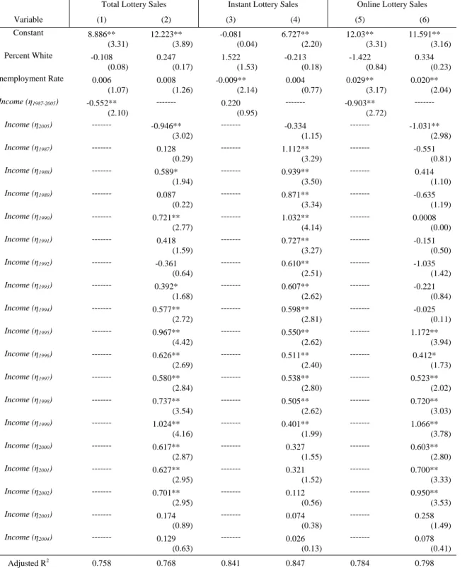
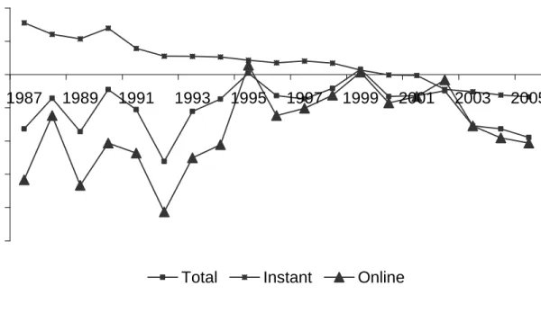
The empirical results for the West Virginia lottery are shown in Table 2.26,27 The calculated annual income elasticities are plotted in Figure 1. The estimated income
24
An income elasticity less than one suggests that the lottery is a normal good and that the lottery tax is regressive, a negative income elasticity suggests an inferior good and a tax that is regressive, and an income elasticity greater than one reflects a luxury good and a tax that is progressive.
25
A history of online games in each state was provided by the respective state lottery agency.
26
The coefficients on the county and year dummy variables are not listed, but will gladly be provided for each regression and each state upon request. The majority of the county and year dummy variable coefficients in the regressions for West Virginia are statistically significant.
elasticities reveal that the West Virginia lottery is regressive and that there are
statistically significant differences in the degree of regressivity over the sample period. In addition, the annual income elasticity estimates are generally different than the sample income elasticity coefficient estimated for specifications (1), (3), and (5).
[Table 2] [Figure 1]
There are differences in the income elasticity of demand for instant and online games, both over time and in a given year. The income elasticities for instant games in early years were not statistically different than one, suggesting that the lottery tax
associated with instant games was initially proportional rather than regressive. However, instant games have become more regressive over time, having annual income elasticities between 0.78 in 1987 and -0.33 in 2005. Online games are generally more regressive (and inferior) than instant games, and the annual income elasticities are more variable than those for instant games in the earlier years of the lottery.28 Online games have become less regressive over time, especially since 1992. As seen in Figure 1, the upward trend in the income elasticity of online games begins in 1992 — the same year PowerBall began. This fact lends some support to Oster’s (2004) finding that a lottery game having a larger jackpot may be less regressive. However, the regressivity of online games has
27
As seen in Table 2, the coefficient on the unemployment rate varies in sign and statistical significance. Because we include income and unemployment in the same regression equation, a change in the
unemployment rate holding income constant reveals how changes in the distribution of county income affect county lottery sales. A negative coefficient on the unemployment rate may reflect an increase in the upper distribution of income, which, if lotteries are regressive, would imply lower sales. We consistently find a negative coefficient on the unemployment rate in the Iowa and Florida regressions presented later.
28
In our prior discussion of studies examining income elasticities over time, we noted that Mikesell (1989) and Jackson (1994) found that the income elasticity for instant games was less than for online games. On the other hand, in addition to our finding, Stover (1987) finds that online games are more regressive (and inferior) than instant games using a sample of U.S. states. Hansen (1995), Hansen et al. (2000), and Price and Novak (1999) also provide evidence that lottery games can be inferior goods. Survey data from the National Opinion Research Council, which is reviewed in Kearney (2005), suggests that instant games are more regressive than online games.
increased after 2002, and the income elasticity of demand for instant games has not noticeably increased as a result of the introduction of higher prize instant games in the 1990s ($2 and $5 instant games were introduced in 1994 and 1998, respectively).
In addition, Figure 1 shows that the income elasticities for instant and online games have become more similar since the mid 1990s. Although we have no a priori expectations on the income elasticities of demand for instant and online games, perhaps one explanation for the apparent convergence of instant and online income elasticities is the addition of two multi-state lottery games to West Virginia’s lottery portfolio – PowerBall in 1992 and Daily Millions in 1996. Iowa has had an identical experience with multi-state game introduction (same games, same years of introduction), so its experience will provide additional evidence for or against this hypothesis.
The Iowa Lottery
The empirical results for the Iowa lottery are shown in Table 3 and the calculated annual income elasticities are plotted in Figure 2. Similar to the West Virginia lottery, the estimated annual income elasticities of demand for the Iowa lottery as a whole are different over time, although statistically significant differences in annual income
elasticities only occur in the early years of the lottery which appears to be less regressive than in later years.29 The computed income elasticities of demand reveal that the Iowa lottery is regressive but less so than the West Virginia lottery. No lottery games in Iowa
29
The majority of the county dummy coefficients in each regression are statistically significant, whereas the year dummy coefficients are not jointly different than zero. Although lacking in statistical significance, we retained the year dummy variables in the Iowa regression equations because omitting them would provide misleading annual income elasticity estimates since the income elasticity estimates are based on the interaction of a year dummy and per capita income. We desire the income elasticity coefficient to only reflect the effect of income changes on sales, not the year effect also.
are (statistically) inferior goods. The trend in instant game income elasticities and
elasticity magnitudes are similar to that of the West Virginia lottery. The introduction of higher priced and higher payout instant lottery tickets in Iowa ($2 in 1992, $3 in 1999, $10 in 2000, and $20 in 2004) resulted in no apparent decrease in the regressivity of instant lottery games, but it is possible that the introduction of higher priced instant games in Iowa (and West Virginia) did slow the increase in regressivity that has occurred over time.
[Table 3] [Figure 2]
Figure 2 reveals that the income elasticities for instant and online games in Iowa have trended down over the period of 1987 to 1997 and then appear to have increased slightly before remaining relatively stable since that time. Based on the statistical significance of the coefficient estimates in Table 3, this downward trend is generally significantly different through 1992 for instant games and the lottery as a whole.
Similar to West Virginia’s experience with multi-state games, Iowa introduced PowerBall in 1992 and Daily Millions in 1996. While the income elasticity of demand for online games in West Virginia appears to have increased at the time these large
jackpot games were introduced, the income elasticity of demand for online games in Iowa has not increased. In fact, none of the pre-2005 income elasticities of demand for online games are statistically different than the 2005 online game income elasticity, which is itself not statistically different than zero. Finally, the relative difference between instant and online income elasticities has remained much more constant over time than in West
Virginia, thus shedding some doubt on the idea that multi-state games might explain the convergence of instant and online income elasticities over time in West Virginia.
The Florida Lottery
The empirical results for the Florida lottery are shown in Table 4 and the calculated annual income elasticities are plotted in Figure 3.30 Similar to the West Virginia lottery and the Iowa lottery, the empirical results and computed annual income elasticities reveal that the Florida lottery is regressive. The regressivity of the lottery as a whole has remained relatively stable over time, decreasing slightly in the late 1990s and early 2000s. The income elasticity of demand for online games has decreased over time. The introduction of higher priced instant games in 1993 ($2 tickets), 1998 ($5 tickets), 2002 ($10 tickets), and 2004 ($20 tickets) had no apparent decrease in the regressivity of instant tickets, as the annual income elasticities of demand for instant games over the period 1990 to 2004 are not statistically different from the 2005 value of 0.617, as is evident from the insignificant income coefficients in specification (4) of Table 4. The 1989 income elasticity of demand for instant games is not statistically different than one. This result, along with similar findings for instant games in West Virginia and Iowa, suggest that instant lottery games were not (statistically) regressive in the early years of the lottery.
30
The majority of the county dummy coefficients in each regression are statistically significant. As with the Iowa lottery, we retained the insignificant year dummy variables to ensure that the annual income coefficients only reflect the effect of income on sales and not also the year effect. The coefficient on percent white was not statistically significant in the West Virginia and Iowa regressions, but it is negative and significant in the Florida specifications. One hypothesis is that the variation in the percent of Florida county population that is white is much greater than in West Virginia and Iowa. For example, the standard deviation of the percent white variable is 0.10 in Florida and only 0.03 and 0.02 in West Virginia and Iowa, respectively.
[Table 4] [Figure 3]
The Florida lottery differs from the lotteries in West Virginia and Iowa in that there are no multi-state lottery games (see Table 1). In addition, the Florida lottery has added only one online game to its online lottery game portfolio since 1991 – Mega Money in 1999. The general decrease in the regressivity of online games appears to have begun in the year or two after 1991. During the mid 1990s the Florida Lotto and Fantasy Five were restructured to generate higher jackpots, possibly explaining the decrease in regressivity for online games during that period. However, the regressivity of the lottery has not continued to (statistically) decrease since the introduction of the final online game in 1999. Finally, the annual income elasticities of demand for instant and online Florida lottery games are more similar over time than those for the West Virginia lottery or the Iowa lottery. One explanation for this is that the Florida lottery has experienced less change in its online games over time than the other two state lotteries.
Further Analysis: Changes in the Gambling Landscape
In this section we explore how the introduction of casino gambling and a state lottery in neighboring states may have changed the income elasticity of demand for lottery tickets in each of our three states. Doing so allows us to explore whether changes in the gambling landscape may have affected the levels of the income elasticities
estimated in the earlier analysis. As discussed earlier, however, if the income elasticity of the border counties changes, then the state’s income elasticity may also change, but not necessarily in the same direction.
We re-estimate equation (1), but replace the annual income elasticity estimates with border county and casino county income elasticities. For each of our three states, we create a border dummy variable for each border state. Counties that border this state are given a value of ‘1’ and a value of ‘0’ otherwise. We then interact this border dummy variable with county income. Because we include per capita income for all counties in the regression, the coefficient on each interaction variable reflects the marginal difference in the income elasticity of demand for lottery tickets in a particular set of border counties relative to internal counties. A similar procedure is done for the counties that have introduced casino gambling, but this coefficient reflects the marginal difference in the income elasticity of demand in casino counties relative to all other counties.
Next, for those border counties that border a state that introduced a lottery after the state of interest, we break the interaction variable into two periods – one period is before the introduction of a lottery in the neighboring state and the other period is after the introduction of a lottery in a neighboring state. Coefficient equality tests will reveal whether there is a significant difference in the (marginal) income elasticity of demand for lottery tickets before and after the introduction of a lottery in a border state. We also break the casino county income elasticity variable into a pre-casino period and a post-casino period to see whether the income elasticity of demand for lottery tickets in post-casino counties has changed after the introduction of casino gambling.
The West Virginia Lottery
The empirical results for West Virginia are shown in Table 5. Of the five states that border West Virginia, Virginia and Kentucky introduced a lottery after West Virginia
introduced its lottery.31 The coefficients on income for the border counties of Ohio, Pennsylvania, and Maryland reveal the marginal difference in the income elasticity of demand for West Virginia lottery tickets in these border counties relative to internal West Virginia counties. This is also true for the counties that border Virginia and Kentucky, but these income coefficients are specific to either the period before border state lottery introduction or after border state lottery introduction.
[Table 5]
From Table 5 we see that the income elasticity of demand in Ohio and
Pennsylvania border counties is significantly different (in most cases higher) than that of internal counties. The results suggest that the West Virginia lottery is regressive for internal counties but is progressive in Ohio and Pennsylvania border counties. These border counties tend to have higher per capita income than the internal counties.
Focusing on the Virginia and Kentucky border county income coefficients, we find that the income elasticities of demand before and after border state lottery
introduction are very similar, but both are quite different than the income elasticity of demand for internal counties. Thus, the introduction of a lottery in a bordering state has not resulted in large changes in the income elasticity of demand for lottery tickets in Virginia and Kentucky border counties, but the income elasticity of demand in these border counties is different (much more regressive) than the income elasticity in internal West Virginia counties. The F-tests for coefficient equality reveal that, in most cases, the income elasticity of demand before border state lottery adoption is significantly different
31
Lottery start dates are: Ohio – August 1974; Kentucky – April 1989; Virginia – September 1988; Maryland – May 1973, Pennsylvania – March 1972; West Virginia – January 1986.
than the income elasticity of demand after border state lottery adoption. It is hard to argue, however, that there is any economic difference in the estimates.
A similar result is found regarding West Virginia casino counties.32 The income elasticity for these counties is significantly smaller (more regressive) than for other counties, yet there appears to be no economic difference in the income elasticity of demand before and after casino introduction (-2.22 versus -2.18, respectively). The F -test does reveal that these two coefficients are statistically different, however.
The Iowa Lottery
The results for the Iowa lottery are shown in Table 6. The income elasticity of demand in Illinois and Missouri border counties are generally larger than that of internal Iowa counties, thus suggesting that the Iowa lottery is less regressive or even progressive (depending upon the coefficient estimate) in these counties relative to internal counties.33
[Table 6]
The states of Nebraska, Minnesota, and Wisconsin adopted a lottery after Iowa. The income elasticity of demand in Nebraska border counties appears to be roughly the same before and after the introduction of the Nebraska lottery (statistically different for total sales and instant sales), although both coefficients suggest that the Iowa lottery is more regressive in Nebraska border counties than in internal counties. A similar result is
32
There are four racinos (casinos at pari-mutuel racetracks) in West Virginia, each in a different county. Two are located in the northern panhandle, one is located in the eastern panhandle, and one is located in the south central part of the state.
33
Lottery start dates are: Nebraska – September 1993; Missouri – January 1986; Illinois – July 1974; Wisconsin – September 1988; Minnesota – April 1990; Iowa – August 1985. Only one county in Iowa borders South Dakota (lottery start date of September 1987), so we did not create a South Dakota border dummy variable. Casino gaming began in Iowa in 1991, but did not become widespread until 1994. We thus chose 1994 as the break-year for our casino county dummy variable. Thirteen counties in Iowa currently have commercial casino gambling.
found for Minnesota border counties, but only for total sales and instant sales. Online games were slightly more progressive (less regressive) in Minnesota border counties prior to the introduction of the Minnesota lottery. The Wisconsin results reveal that the income elasticity of demand in Wisconsin border counties is no different than that of internal counties, and no significant difference exists in these counties before and after the introduction of the Wisconsin lottery (except online sales prior to the Wisconsin lottery, which is quite small).
The income elasticity of demand in Iowa casino counties is less than in other Iowa counties. But, there appears to be no economic difference in the income elasticity of demand for lottery tickets in casino counties before and after the introduction of casino gaming in those counties. There is a statistically significant difference in these
coefficients for total lottery sales and online lottery sales, however.
The Florida Lottery
The results for Florida are shown in Table 7.34 The income elasticity of demand in Alabama border counties is much lower than in internal counties. We find that the income elasticity of demand in Georgia border counties is slightly smaller after the introduction of the Georgia lottery than before, but, as in the case of West Virginia and Iowa, the difference is not of any economic significance. There also appears to be no meaningful difference in the income elasticity of demand in casino counties before and after the introduction of casino gambling, but the income elasticity of demand is lower in
34
The Florida lottery began January 1988 and the Georgia lottery began June of 1993. Five counties in Florida have either Native American gambling or racinos.
casino counties relative to non-casino counties regardless of the presence of a casino. This result also mimics the findings for West Virginia and Iowa.
[Table 7]
Discussion and Concluding Comments
Some general conclusions regarding the dynamic nature of the income elasticity of demand for lottery tickets can be made from the empirical results presented in the previous sections:
• The income elasticity of demand for lottery tickets changes over time. This suggests that empirical estimates of income elasticities using a single cross-section or a single estimate from panel will not accurately reflect the income elasticity of demand over time.
• There is some evidence that large jackpot games, such as multi-state games, decrease (or at least stop the increase in) the regressivity of online lottery games. The results are less clear regarding this possibility for instant games, which tend to become more regressive (or at least not less regressive) over time.
• On average, the regressivity of online games appears to be equal or greater than the regressivity of instant games for the three states studied. This result contrasts with Mikesell’s (1989) finding for Illinois that the income elasticity for online games tended to be less than that for instant games, but does support Stover (1987) who finds that online games are more regressive than instant games in a sample of U.S. states. The instant game tax burden appears to be proportional rather regressive in the early years of the lottery.
• There is some evidence that the income elasticities of demand for instant and online games converge after a state’s online lottery product line has remained similar from some time.
• Not only do the income elasticities change over time for a specific state, but the relative difference in the degree of regressivity for each state’s lottery as a whole is ranked with the income level of each state.35 West Virginia lottery is the most regressive and the state has the lowest per capita income of the three states. The Florida lottery is the least regressive and the state has the highest per capita income of the three states. Iowa lies between West Virginia and Florida in terms of lottery regressivity and per capita income.36
• Changes in the gambling landscape external to the state lottery have had little effect on the income elasticity of demand for lottery tickets. The introduction of a lottery in a neighboring state has little impact on the income elasticity of demand for tickets in border counties. In general, for the three states studied here, the income elasticity is slightly smaller after the introduction of a lottery in neighboring states, but the economic significance of this difference is slight at most. Thus, lottery game
35
Different income elasticities across the states should not be too surprising. For any individual consumer (which we approximate using county-level data), the income elasticity of demand for a product is
(∂x/∂y)·(y/x), where x = quantity of a good and y = income. Ignoring the second part of the product for simplicity, equal income elasticities across consumers implies that the marginal propensity to consume lottery tickets is the same for all consumers (i.e. ∂x/∂y is the same for all consumers). This is highly unlikely given that consumers are heterogeneous, especially across counties and states. In addition, equal marginal propensities to consume also implies that the propensities to consume out of different income sources (transfer payments, earnings, etc. is the same). Numerous studies have shown that the marginal propensities to consume out of different income sources are not the same (Carriker et al., 1993; Holbrook and Stafford, 1971; Hymans and Shapiro, 1976). Thus, we attribute differences in income elasticities across the states to heterogeneous consumers, difference in lottery games across the states, and differences in propensities to consume out of different income sources (which vary across counties and states).
36
For the period 1992 to 2005, the average of annual per capita income for the three states is: West Virginia - $21,376; Iowa - $24,485; Florida - $27,246.
introduction in bordering states is unlikely to have significantly changed the income elasticity of demand for tickets in the home state.
• The trends in the income elasticity of demand over time likely reflect the general growth in consumer income and changes to the home state lottery portfolio rather than any significant economic effects from casino gambling or lottery introduction in neighboring states.
Several points follow from our empirical results regarding changing income elasticities over time. The regressivity of state lotteries has been (and likely will continue to be) the greatest argument against them. Although one can take the view that
regressivity is bad regardless of the degree of regressivity, we argue that there is a significant difference in the policy discussion of state lotteries with regards to a lottery having an income elasticity of, say, 0.20 versus 0.90. Certainly the weight of the regressivity argument is dependent upon the degree of regressivity rather than absolute regressivity, and, as shown here, the degree of regressivity can change over time. Thus, any serious policy discussion regarding the regressivity of state lotteries and the
respective costs and benefits of state lotteries should consider the dynamic nature of lottery tax burdens over time rather than rely on a static income elasticity estimate.
One interesting feature of our analysis is that the annual income elasticity estimates allow an examination of whether the income elasticity of demand for lottery tickets is sensitive to economic conditions. One expectation is that the business cycles in the individual states and counties, which are distinctive to each state and county, should affect lottery sales (Mikesell, 1994). For the years in which real per capita income
growth is less than one percent, none of the estimated annual income elasticities appear to be driven by weak economic conditions.37 We find no evidence that the income elasticity of demand for lottery tickets is different in recession and non-recession years.
Our results have several implications for the revenue prospects of states lotteries. First consider the long term revenue potential of each state’s lottery. The estimated income elasticities of demand for the three states studied here suggest that lottery revenue growth will be much less than income growth. For every year for each state, the point estimates for our income elasticities are less than one. Moreover, we find no evidence that the income elasticity is likely to increase over time so that it would exceed one.
In fact, the income elasticities for West Virginia are negative, so income growth should lead to a decline in per capita lottery revenue over time. As evidence, real per capita lottery revenues in West Virginia peaked in 1999. The annual income elasticities for the Iowa lottery are near zero for recent years, so income growth is likely to generate little growth in Iowa lottery revenue. Again, as evidence, real per capita lottery revenues in Iowa have been roughly constant since 1977. The revenue prospects of the Florida lottery are the most favorable. The income elasticities have been near 0.5 in recent years, so per capita income growth should produce lottery revenue increases at a rate greater than that of Iowa and West Virginia, although a given increase in per capita income will generate a less than proportionate increase in per capita lottery revenue.38 A more optimistic assessment can be reached by focusing on Florida’s recent experience.
37
Our use of annual data is far from ideal in capturing business-cycle effects. The coefficients on the year dummy variables (not shown) show no evidence of any business cycle effects.
38
Similarly, population changes also have also been unfavorable for lottery revenue growth. West
Virginia’s population in 2005 was less than in 1987; however, population growth has been slightly positive since 2001. Positive population growth has occurred in Iowa, but at a slower pace than the United States as a whole. Of the three states, Florida has experienced the greatest population growth population growth substantially faster than the United States as a whole.
Between 2001 and 2005 the growth of real per capita lottery spending exceeded that of real per capita income. However, a slightly longer perspective reveals that real per capita lottery spending was lower in 2005 than in 1994. Admittedly, the introduction of new lottery products might increase substantially the income elasticity of lottery demand and/or generate consistent upward shifts in lottery spending in counties throughout a state. Based on our estimates and past spending on lotteries, there is little, if any, reason to anticipate such a scenario on a sustained basis.
A related issue is the potential growth of lottery revenues relative to the revenue growth potential from other significant state taxes, such as personal income, corporate income, retail sales, and motor fuels. These tax bases typically have income elasticities near one, except in the case of retail sales which is less than one but still greater than 0.5 and corporate income which is around 3.0 (Holcombe and Sobel, 1996, 1997). These income elasticity estimates are somewhat larger than the income elasticity of lottery demand estimates found here and in prior lottery studies.39 Assuming relatively stable tax bases, this suggests that the growth potential of state lotteries with respect to income growth is much less than for traditional sources of revenue. On the other hand, lottery revenues will not fall as much as revenues from traditional sources in an economic slowdown. The former may explain state lottery agencies’ continual updates of their lottery portfolios to increase consumer participation. The fact that we find decreasing income elasticities over time suggests that, at least for the states and games studied here, lottery revenues have become a relatively more stable (with respect to changes in
income) source of revenue than traditional revenue sources.
39
One caveat is that most lottery demand studies have used cross-sectional data, whereas Holcombe and Sobel (1996, 1997) used time series data. Mikesell (1994) estimated an income elasticity of demand around 3.0 in his panel study of state-level lottery sales.
Table 1: Online Lottery Game History
WEST VIRGINIA LOTTERY
Online Games Start Date End Date Multi-State Game
Daily 3 Feb-87 No
Daily 4 Feb-87 No
Cash 25 Feb-90 No
Travel Keno Dec-92 No
Lotto Dec-86 Jan-90 No
Daily Millions Sep-96 Mar-98 Yes
(replaced with Cash 4 Life) Mar-98 Sep-00 Yes
(replaced with Rolldown) Sep-00 Apr-02 Yes
(replaced with Hot Lotto) Apr-02 Yes
Lotto America Feb-88 Apr-92 Yes
(replaced with PowerBall) Apr-92 Yes
IOWA LOTTERY
Online Games Start Date End Date Multi-State Game
Iowa Lotto May-86 Oct-93 No
Pick 3 Jul-98 No
Pick 4 Sep-03 No
Freeplay Replay Mar-00 Sep-03 No
Daily Deal Feb-91 Jan-92 No
$100,000 Daily Cash Jan-92 No
Lucky Day Oct-93 Oct-94 No
Super Cash Oct-94 Jun-98 No
Dream Draw Jun-96 Nov-96 No
Daily Millions Sep-96 Mar-98 Yes
(replaced with Cash 4 Life) Mar-98 Nov-00 Yes
(replaced with Rolldown) Sep-00 Apr-02 Yes
(replaced with Hot Lotto) Apr-02 Yes
Lotto America Feb-88 Apr-92 Yes
(replaced with PowerBall) Apr-92 Yes
FLORIDA LOTTERY
Online Games Start Date End Date Multi-State Game
Florida Lotto Apr-88 No
Cash 3 Apr-88 No
Fantasy 5 Apr-89 No
Play 4 Jul-91 No
Mega Money May-99 No
Note: Game histories provided by lottery agencies. See text for start dates for higher priced instant lottery tickets.
Table 2 – Regression Results: West Virginia Lottery
Total Lottery Sales Instant Lottery Sales Online Lottery Sales
Variable (1) (2) (3) (4) (5) (6) Constant 8.886** (3.31) 12.223** (3.89) -0.081 (0.04) 6.727** (2.20) 12.03** (3.31) 11.591** (3.16) Percent White -0.108 (0.08) 0.247 (0.17) 1.522 (1.53) -0.213 (0.18) -1.422 (0.84) 0.334 (0.23) Unemployment Rate 0.006 (1.07) 0.008 (1.26) -0.009** (2.14) 0.004 (0.77) 0.029** (3.17) 0.020** (2.04) Income (η1987-2005) -0.552** (2.10) --- 0.220 (0.95) --- -0.903** (2.72) --- Income (η2005) --- -0.946** (3.02) --- -0.334 (1.15) --- -1.031** (2.98) Income (η1987) --- 0.128 (0.29) --- 1.112** (3.29) --- -0.551 (0.81) Income (η1988) --- 0.589* (1.94) --- 0.939** (3.50) --- 0.414 (1.10) Income (η1989) --- 0.087 (0.22) --- 0.871** (3.34) --- -0.635 (1.19) Income (η1990) --- 0.721** (2.77) --- 1.032** (4.14) --- 0.0008 (0.00) Income (η1991) --- 0.418 (1.59) --- 0.727** (3.27) --- -0.151 (0.50) Income (η1992) --- -0.361 (0.64) --- 0.610** (2.51) --- -1.035 (1.42) Income (η1993) --- 0.392* (1.68) --- 0.607** (2.62) --- -0.221 (0.84) Income (η1994) --- 0.577** (2.72) --- 0.598** (2.81) --- -0.025 (0.11) Income (η1995) --- 0.967** (4.42) --- 0.550** (2.62) --- 1.172** (3.94) Income (η1996) --- 0.626** (2.69) --- 0.511** (2.40) --- 0.412* (1.73) Income (η1997) --- 0.580** (2.84) --- 0.538** (2.80) --- 0.523** (2.02) Income (η1998) --- 0.737** (3.54) --- 0.505** (2.62) --- 0.720** (3.03) Income (η1999) --- 1.024** (4.16) --- 0.401** (1.99) --- 1.066** (3.78) Income (η2000) --- 0.617** (2.87) --- 0.327 (1.55) --- 0.603** (2.80) Income (η2001) --- 0.627** (2.95) --- 0.321 (1.52) --- 0.700** (3.33) Income (η2002) --- 0.701** (2.95) --- 0.112 (0.56) --- 0.950** (3.53) Income (η2003) --- 0.174 (0.89) --- 0.074 (0.38) --- 0.258 (1.49) Income (η2004) --- 0.129 (0.63) --- 0.026 (0.13) --- 0.078 (0.41) Adjusted R2 0.758 0.768 0.841 0.847 0.784 0.798 Observations 1045 1045 1045 1045 1045 1045
Note: Absolute t-statistics are in parentheses and were computed using White’s heteroscedasticity-corrected standard errors. * denotes significance at 10 percent, ** denotes significance at 5 percent or better. County and year dummy variables are included in each specification. The income elasticity estimates for 1987 to 2004 are each relative to the income elasticity for 2005. Sample period is 1987 to 2005 for 55 counties.
Table 3 – Regression Results: Iowa Lottery
Total Lottery Sales Instant Lottery Sales Online Lottery Sales
Variable (1) (2) (3) (4) (5) (6) Constant 2.084 (1.51) 4.275** (2.05) 0.193 (0.12) 3.403 (1.44) 2.902** (1.96) 3.130 (1.39) Percent White 0.146 (0.15) -1.101 (1.04) 1.556 (1.38) 0.066 (0.06) -1.533 (1.44) -2.200* (1.93) Unemployment Rate -0.028** (4.89) -0.026** (4.55) -0.030** (4.66) -0.028** (4.26) -0.020** (3.32) -0.020** (3.19) Income (η1987-2005) 0.158 (1.51) --- 0.171 (1.44) --- 0.122 (1.09) --- Income (η2005) --- 0.057 (0.32) --- -0.011 (0.06) --- 0.166 (0.86) Income (η1987) --- 0.582** (2.33) --- 0.674** (2.37) --- 0.385 (1.43) Income (η1988) --- 0.419* (1.87) --- 0.560** (2.20) --- 0.125 (0.52) Income (η1989) --- 0.294 (1.23) --- 0.246 (0.91) --- 0.257 (1.00) Income (η1990) --- 0.389 (1.63) --- 0.506* (1.86) --- 0.117 (0.46) Income (η1991) --- 0.474** (2.03) --- 0.693** (2.62) --- 0.052 (0.21) Income (η1992) --- 0.375 (1.58) --- 0.533** (1.98) --- 0.072 (0.28) Income (η1993) --- 0.183 (0.86) --- 0.295 (1.22) --- -0.003 (0.01) Income (η1994) --- 0.166 (0.71) --- 0.298 (1.12) --- -0.014 (0.06) Income (η1995) --- 0.074 (0.36) --- 0.230 (0.98) --- -0.188 (0.84) Income (η1996) --- 0.048 (0.22) --- 0.173 (0.69) --- -0.184 (0.78) Income (η1997) --- -0.041 (0.18) --- 0.047 (0.18) --- -0.164 (0.67) Income (η1998) --- 0.002 (0.01) --- 0.052 (0.21) --- -0.006 (0.03) Income (η1999) --- -0.089 (0.41) --- -0.099 (0.41) --- 0.005 (0.02) Income (η2000) --- 0.042 (0.19) --- 0.096 (0.38) --- 0.005 (0.02) Income (η2001) --- 0.031 (0.15) --- 0.087 (0.36) --- -0.083 (0.36) Income (η2002) --- 0.146 (0.68) --- 0.197 (0.81) --- -0.007 (0.03) Income (η2003) --- 0.121 (0.58) --- 0.212 (0.89) --- -0.067 (0.30) Income (η2004) --- 0.159 (0.72) --- 0.199 (0.80) --- 0.043 (0.18) Adjusted R2 0.835 0.835 0.826 0.826 0.839 0.838 Observations 1862 1862 1862 1862 1862 1862
Note: Absolute t-statistics are in parentheses. * denotes significance at 10 percent, ** denotes significance at 5 percent or better. County and year dummy variables are included in each specification. The income elasticity estimates for 1987 to 2004 are each relative to the income elasticity for 2005. Sample period is 1987 to 2005 for 98 counties.
Table 4 – Regression Results: Florida Lottery
Total Lottery Sales Instant Lottery Sales Online Lottery Sales
Variable (1) (2) (3) (4) (5) (6) Constant 1.777 (1.12) 3.072* (1.79) 0.041 (0.03) 0.274 (0.18) 0.321 (0.20) 0.591 (0.34) Percent White -2.480** (3.90) -2.65** (4.14) -1.921** (3.41) -2.10** (3.64) -3.845** (6.14) -3.01** (4.80) Unemployment Rate -0.011* (1.93) -0.009 (1.56) -0.010** (2.01) -0.008 (1.58) -0.012** (2.03) -0.012** (2.12) Income (η1989-2005) 0.502** (2.99) --- 0.627** (4.34) --- 0.635** (3.61) --- Income (η2005) --- 0.380** (2.14) --- 0.617** (3.95) --- 0.530** (2.93) Income (η1989) --- 0.188* (1.66) --- 0.186* (1.63) --- -0.265** (2.36) Income (η1990) --- 0.178 (1.45) --- 0.104 (0.85) --- -0.299** (2.58) Income (η1991) --- 0.132 (1.06) --- 0.039 (0.35) --- -0.302** (2.46) Income (η1992) --- 0.040 (0.32) --- -0.112 (1.00) --- -0.351** (2.80) Income (η1993) --- 0.093 (0.78) --- -0.084 (0.82) --- -0.270** (2.19) Income (η1994) --- 0.156 (1.63) --- -0.029 (0.35) --- -0.167* (1.72) Income (η1995) --- 0.152* (1.71) --- -0.070 (0.86) --- -0.132 (1.52) Income (η1996) --- 0.173* (1.92) --- 0.037 (0.44) --- -0.071 (0.83) Income (η1997) --- 0.213** (2.37) --- 0.047 (0.58) --- -0.041 (0.48) Income (η1998) --- 0.154* (1.65) --- 0.012 (0.15) --- -0.081 (0.89) Income (η1999) --- 0.215** (2.16) --- -0.0006 (0.01) --- -0.019 (0.19) Income (η2000) --- 0.269** (2.62) --- -0.004 (0.05) --- 0.077 (0.74) Income (η2001) --- 0.230** (2.03) --- 0.007 (0.07) --- 0.053 (0.46) Income (η2002) --- 0.199* (1.65) --- -0.020 (0.18) --- 0.047 (0.40) Income (η2003) --- 0.086 (0.73) --- -0.022 (0.23) --- 0.024 (0.20) Income (η2004) --- 0.003 (0.03) --- -0.053 (0.58) --- -0.014 (0.12) Adjusted R2 0.843 0.843 0.883 0.883 0.906 0.910 Observations 1139 1139 1139 1139 1139 1139
Note: Absolute t-statistics are in parentheses and were computed using White’s heteroscedasticity-corrected standard errors. * denotes significance at 10 percent, ** denotes significance at 5 percent or better. County and year dummy variables are included in each specification. The income elasticity estimates for 1989 to 2004 are each relative to the income elasticity for 2005. Sample period is 1989 to 2005 for 67 counties.
Table 5 – New Lottery and Casino Gambling: Effect on Income Elasticity of Demand West Virginia Lottery
Variable Total Sales
(1)
Instant Sales (2)
Online Sales (3)
Income (η) - All counties in West Virginia -0.097
(0.41)
0.512** (2.35)
-0.467 (1.53)
Income (η) – OH border counties 0.660**
(2.54)
-0.641** (2.67)
2.064** (6.51)
Income (η) – PA border counties 1.029**
(3.46)
0.328 (1.36)
1.033** (3.06)
Income (η) – MD border counties -0.102
(0.27)
-0.413 (1.43)
0.495 (0.93)
Income (η) – VA border counties < 1989 -0.379
(1.59)
-0.505** (2.08)
-0.154 (0.50)
Income (η) – VA border counties ≥ 1989 -0.410*
(1.77)
-0.545** (2.27)
-0.183 (0.62)
Income (η) – KY border counties < 1990 -2.401**
(2.55)
-2.446** (3.28)
-1.926* (1.83)
Income (η) – KY border counties ≥ 1990 -2.430**
(2.63)
-2.484** (3.39)
-1.962* (1.90)
Income (η) – Casino counties < 1995 -2.222**
(4.88)
-0.863** (3.07)
-2.812** (4.82)
Income (η) – Casino counties ≥ 1995 -2.180**
(4.86) -0.877** (3.15) -2.744** (4.77) Adjusted R2 0.79 0.87 0.81 Number of Observations 1045 1045 1045 F-test: H0: VA<1989 = VA≥1989 18.96** 48.10** 8.36** F-test: H0: KY<1990 = VA≥1990 3.14* 8.37** 2.50
F-test: H0: Casino<1995 = Casino≥1995 23.11** 4.04** 32.61**
Note: Absolute t-statistics are in parentheses. * denotes significance at 10 percent, ** denotes significance at 5 percent or better. County and year dummy variables are included in each specification, along with a constant term, the unemployment rate, and the percent white. Sample period is 1987 to 2005. Complete regression results will be provided upon request.
Table 6 – New Lottery and Casino Gambling: Effect on Income Elasticity of Demand Iowa Lottery
Variable Total Sales
(1)
Instant Sales (2)
Online Sales (3)
Income (η) - All counties in Iowa 0.240**
(2.12)
0.244* (1.94)
0.224* (1.93)
Income (η) – IL border counties 1.349**
(6.17)
0.259 (1.06)
2.908** (12.92)
Income (η) – MO border counties 0.499**
(3.18)
0.521** (2.99)
0.438** (2.71)
Income (η) – NE border counties < 1994 -0.645**
(2.33)
-0.593* (1.93)
-0.745** (2.61)
Income (η) – NE border counties ≥ 1994 -0.656**
(2.41)
-0.605** (2.00)
-0.749** (2.67)
Income (η) – MN border counties < 1991 -0.001
(0.16)
-0.052** (7.31)
0.066** (9.99)
Income (η) – MN border counties ≥ 1991 -0.047**
(7.90)
-0.091** (13.79)
0.009 (1.45)
Income (η) – WI border counties < 1989 0.008
(0.58)
0.005 (0.30)
0.026* (1.73)
Income (η) – WI border counties ≥ 1989 0.004
(0.32)
0.009 (0.50)
-0.005 (0.36)
Income (η) – Casino counties < 1994 -0.518**
(2.48)
-0.460** (1.98)
-0.682** (3.17)
Income (η) – Casino counties ≥ 1994 -0.510**
(2.47) -0.456** (1.99) -0.668** (3.14) Adjusted R2 0.83 0.83 0.85 Number of Observations 1881 1881 1881 F-test: H0: NE<1994 = NE≥1994 3.61* 3.53* 0.46 F-test: H0: MN<1991 = MN≥1991 211.25** 124.84** 303.08** F-test: H0: WI<1989 = WI≥1989 0.31 0.25 14.38**
F-test: H0: Casino<1994 = Casino≥1994 4.50** 1.11 14.79**
Note: Absolute t-statistics are in parentheses. * denotes significance at 10 percent, ** denotes significance at 5 percent or better. County and year dummy variables are included in each specification, along with a constant term, the unemployment rate, and the percent white. Sample period is 1987 to 2005. Complete regression results will be provided upon request.