A Tax on Tax Revenue. The Incentive Effects of Equalizing Transfers: Evidence from Germany

September 2000

CESifo

Poschingerstr. 5

81679 Munich

Germany

Phone: +49 (89) 9224-1410/1425

Fax: +49 (89) 9224-1409

http://www.CESifo.de

________________________

* We would like to thank Claus Schnabel, Thiess Büttner, Regina Riphahn and Jörg Breitung for very helpful comments on an earlier draft of this paper. The usual disclaimer applies. The third author would like to acknowledge financial support from the informedia-Stiftung, Cologne, through the research program “Efficiency and Justice”.

A TAX ON TAX REVENUE

THE INCENTIVE EFFECTS OF EQUALIZING

TRANSFERS: EVIDENCE FROM GERMANY

Christian Baretti

Bernd Huber

Karl Lichtblau*

Working Paper No. 333

A TAX ON TAX REVENUE

THE INCENTIVE EFFECTS OF EQUALIZING TRANSFERS:

EVIDENCE FROM GERMANY

Abstract

Several recent studies suggest that equalizing transfers in a federal system may distort the tax policy decisions of states. We study this issue for the German federal fiscal system. In a simple theoretical model, we first identify a substitution and an income effect of equalizing transfers. Our main hypothesis is that both effects should tend to reduce tax revenue of German states. We perform various empirical tests which confirm this hypothesis.

JEL Classification: H72, H77

Christian Baretti

Ifo Institute for Economic Research Poschingerstr. 5 81679 Munich Germany Bernd Huber University of Munich Department of Economics Ludwigstr. 28/VG 80539 Munich Germany e-mail: huber.office@lrz.uni-muenchen.de Karl Lichtblau

Cologne Institute for Business Research (IW) 50968 Cologne

1. Introduction

A stylized feature of a federal system is the existence of intergovernmental transfers. Several types of transfers can be distinguished. The federal government (or, more generally, a higher level

government) often pays transfers to support certain spending programs of lower-level governments. These transfers can either take the form of matching or block grants. Much of the recent literature has studied the effects of this type of transfer policy. For example, there now exists an extensive theoretical and empirical literature on the effects of matching versus block grants.1

But, in many federalist countries, one can also observe equalizing transfers which attempt to reduce revenue disparities between sub-federal governments of the same level. A system of equalizing transfers can be found, for example, in Australia, Canada and Germany. In these countries sub-federal governments with below-average tax revenue receive some additional funds. For example, under the “representative tax system” in Canada, the federal government pays transfers to provinces whose tax revenue is below the average (per capita) tax revenue of (a representative sample of) provinces.

Recent theoretical work (Smart (1998), Smart/Bird (1996)) suggests that the existence of equalizing transfers may have important effects on the behavior of sub-level governments. In particular, this literature shows that, under the Canadian system, equalizing transfers will raise the tax rates chosen by poor provinces. The underlying intuition is simply that the negative effects of higher tax rates on a province’s tax base are partly compensated by higher equalizing transfers from the federal

government. More generally, this suggests that equalizing transfers may distort regional decisions and may give rise to fiscal externalities between various levels of government.

The purpose of this paper is to further analyze the effects of equalizing transfers on sub-federal governmental behavior. We study the case of Germany where equalizing transfers play an important role. Germany’s federal system differs in many respects from the system in the United States and Canada. For our analysis, the following features are particularly important. First, the federal

government and the states (Länder) take part in an extensive system of equalizing transfers which we describe in more detail below. Second, taxes, i.e. tax rates and the definition of tax bases, are

1

determined by federal law and are, therefore, uniform across states. While states cannot independently levy taxes, they are however responsible for collecting taxes.

In Germany, as in other federalist countries, higher tax revenue in a state reduces the amount of equalizing transfers received by this state. Intuitively, this decline in equalizing transfers can be interpreted as a tax on a state’s tax revenue. Conceptually, one can then define a marginal tax rate which measures the fraction of additional tax revenue in this state flowing out of the region. The basic idea of our paper is then as follows. Given that German states administer tax collection, suppose now that the amount of tax revenue collected in a state depends on the enforcement activity undertaken by the government of this state. Conventional economic theory suggests that, other things being equal, a state’s level of tax enforcement and thus tax revenue will be lower the higher the marginal tax rate on its tax revenue. In our empirical analysis, we examine how these marginal tax rates affect states’ tax revenue. Germany’s federal system allows us to identify these effects since marginal tax rates substantially vary across states. For example, the marginal tax rates on income tax revenue in 1998 range between 43 % (Schleswig-Holstein) and 92 % (Saarland).

Our main result is that the marginal tax rates imposed by the equalization system have a significantly negative effect on states’ tax revenue. This indicates that equalizing transfers have a negative impact on tax enforcement and, thus, distort states’ fiscal decisions. Furthermore, we also find that the total amount of transfers has a negative effect on tax revenue. Again, this is in line with theoretical

considerations where this response can be explained by an income effect.

The remainder of this paper is organized as follows. Section 2 provides a brief overview over the key features of Germany’s federal system. Section 3 develops the theoretical framework. The empirical analysis is contained in sections 4 and 5. Conclusions are given in section 6.

2. Germany’s Fiscal Equalization System: A Brief Overview

In this section, we provide a brief survey of some key elements of Germany’s fiscal equalization system which was introduced in 1969.2 For our further analysis, the following aspects are important. As was mentioned above, tax legislation is highly centralized at the federal level. In practice, nearly all taxes are determined by federal tax laws.3 Notice that this even applies to taxes whose proceeds exclusively accrue to states. In other words, taxes (tax bases, tax rates) are completely harmonized across states. This also implies that, in what follows, we need not take into account tax policy choices of states concerning tax rates and tax bases. This will considerably simplify our empirical analysis.

While states have no degree of freedom to choose tax rates and tax bases, they have substantial discretion over the administration of taxes. In Germany, all taxes are administered and collected by the states. Notice that states also collect the taxes for the federal government and, thus, effectively serve as an agent for the federal government in this respect.

How is the tax revenue of German states determined? About 25 % of states’ total tax revenue comes from own-source taxes which, like e.g. inheritance taxes, solely accrue to the states. But, the main source of revenue are taxes whose proceeds are shared among federal, state and local governments. These shared taxes are comprised of the VAT, the income tax and the corporate tax. For example, the federal government and the states each receive 42.5 % of total income tax revenue while the share of local governments is 15 %. Similar sharing rules apply to VAT and the corporate tax. The allocation of (the states’ 42.5 % of) income tax revenue to states is determined by the residence of taxpayers, i.e. the revenue accrues to the state where the taxpayer resides. The

distribution of corporate tax revenue is based on a formula apportionment scheme while the states’ share of VAT revenue is allocated on a per capita base.

These rules determine an initial allocation of tax revenue. Table 1 provides an overview of per capita tax revenue in the sixteen German states in 1998. The main purpose of Germany’s fiscal equalization system ((sekundärer) Finanzausgleich) is the redistribution of tax revenue in favor of ”poor” states. One interesting feature of Germany’s system is that, in contrast to the U.S. or many other federalist

2

See also Wurzel (1999) and Huber/Lichtblau (1998).

3

countries, there is an explicit redistribution of tax revenue between states such that ”rich” states pay transfers to ”poor” states. In addition, ”poor” states also receive federal grants. The fiscal

equalization system proceeds in three steps. The first two stages concern the (horizontal)

redistribution between states while federal grants to ”poor” states are determined at the last stage.

At stage 1 (‘Umsatzsteuervorwegausgleich’), up to 25 % of states’ VAT revenue is used to ensure that each state receives 92 % of average per capita tax revenue of all states.4 Due to reunification, VAT redistribution has substantially increased and has become a major source of revenue for the states in former Eastern Germany (see Table 1).

Stage 2 (‘Länderfinanzausgleich im engeren Sinne’) represents a complex system of transfers between the states. The basic idea of this interstate equalization system is to compare a state’s fiscal resources (‘Finanzkraft’) to its fiscal needs (‘Finanzbedarf’). If a state’s fiscal resources are lower than its fiscal needs, it receives transfers, if they are higher it has to pay contributions which finance the transfer payments of the system. How are fiscal resources and fiscal needs determined? Fiscal resources of a state are its tax revenue (including stage 1 redistribution), plus roughly 50 % of the tax revenue of its local governments. Roughly speaking, fiscal needs are a measure of average fiscal resources of all states. Leaving out some further complicating details, a state’s fiscal needs are calculated as average per capita fiscal resources of all states times the population of this state.5

Contributions and transfers are then determined according to a progressive schedule which is based on a state’s relative divergence of its fiscal resources from its fiscal needs. For example, marginal contribution rates vary between 15 % and 80 %. A complex adjustment mechanism ensures that total contributions of ”rich” states equal the amount of transfers received by ”poor” states. Table 1 shows per capita transfers and contributions in 1998. In practice, the current system ensures that “poor” states obtain at least 95 % of average fiscal resources of all states.

At stage 3 (‘Fehlbetragsbundesergänzungszuweisungen’), the federal government pays equalization transfers to ”poor” states. More specifically, ”poor” states receive federal grants (type I) which

4

Local government revenue is not taken into account at this stage.

5

The exact scheme is more complicated since it also uses population weights. In particular, the population in the city states Berlin, Bremen and Hamburg is weighted with the factor 1.35. This also explains the above average tax revenue of these states in table 1.

cover (at least) 90 % of any remaining gap between fiscal resources and fiscal needs. Since poor states already obtain 95 % of average fiscal resources through the interstate equalization system this means that they effectively end up with 99.5 % of average fiscal resources.

In addition, the federal government pays various block grants to states

(‘Sonderbedarfsbundesergänzungszuweisungen’). The bulk of these transfers (federal grants type II) is received by the states in Eastern Germany.

From table 1, one can see that Germany’s fiscal equalization system achieves a considerable redistribution of tax revenue. To gain some insight into the economic effects of this system, we calculate the marginal tax rates which this system imposes on a state’s income tax revenue. The marginal tax rate (MTR) is defined as the fraction of 1 DM of additional income tax revenue in a state which flows out of the region. Table 2 presents the marginal tax rate on states’ income tax revenue for each state in 1998.6 For “poor” states, the MTRs are positive and – for some states – quite high since higher tax revenue in a “poor” state reduces the amount of transfers received through the fiscal equaliziation system. The MTRs of “rich” states reflect that contributions to VAT

redistribution and to the interstate equalization system increase if the tax revenue of a “rich” state rises. The MTRs substantially vary across states. They tend to be lower for ”rich” states like, e.g., Bavaria. Furthermore, the MTR tends to be higher for states with a lower population. This reflects a common pool effect of the interstate equalization system which arises since small states only account for a small fraction of total fiscal resources. Finally, the progressive schedule of the interstate

equalization affects the MTR. For example, the low MTR of Schleswig-Holstein reflects that this state faces a low marginal contribution rate in the interstate equalization system.7

6

See Huber/Lichtblau (1998). These results are based on a simulation which will be discussed in more detail in section 5.

7

This is so since Schleswig-Holstein’s fiscal revenues are only slightly higher than its fiscal needs such that a contribution rate of only 15 % applies.

3. The Theoretical Framework

Table 2 indicates that the MTRs imposed by the German federal system are quite high. As was mentioned in the introduction, this suggests that the MTRs may have a negative effect on the

incentives of German Länder to efficiently administer and collect taxes. This basic idea can be made more precise in a simple model which serves as a theoretical benchmark for our empirical analysis.

Consider a state i in a federalist country with n states. Suppressing state-specification notation, utility

U of the representative private agent in a state is U =u c l

( )

, +h g

( )

where c and l denote private consumption and labor supply, respectively. g is a (regional) public good provided by the state government. Before-tax income y, i.e. output in the region, is given by y y l=

( )

, wherey

( )

⋅ is increasing and strictly concave in l. Income y is taxed at the proportional rate t. To study the German situation, suppose that this tax rate is determined by federal law and cannot be varied by the state. But, we assume that the effective tax rate and the actual tax payment depend on the enforcement activity of the state government which (as in Germany) is responsible for collecting taxes. We follow the approach developed in Bordignon/Manasse/Tabellini (1996) to model the effects of enforcement activity on tax revenue. We consider the simple case of a linear relationship between enforcement activity and actual tax payments. More specifically, we denote by aty the actual tax payment of the private agent where the parameter a denotes the level of enforcement activity which is controlled by the state government. It is plausible that there exists a lower bounda and an upper bound a for the enforcement parameter a. In what follows, we will however assume that neither of these two constraints is binding at a state’s optimum.

Maximization of the household’s utility subject to the private sector budget

constraintc = −

(

1 at y l

) ( )

allows us to derive indirect utilityv

(

1−at

)

+h g

( )

and the output supply function y

(

1−at

)

. Under mild assumptions, y is an increasing function in the tax factor 1 – at.

Consider now the budget of the government of this state. To capture tax sharing between the state and the federal government in Germany, denote by (1 – s) the fraction of tax revenue accruing to the federal government. Tax revenue T of the state then amounts to T = saty(1-at). The equalization system is modelled in a very simple way. Suppose that a state’s transfer is proportional to the

thus would pay contributions, while it receives transfers if T T< .Total transfers or contributions are given by B d T T=

(

−

)

where d is the (proportional) subsidy or contribution rate of the system with

0≤ <d 1. The budget constraint of the state government is thus

(

)

g = −1 d T d T+ (1)

The problem of the state government is then to maximize the agent’s indirect utility function subject to (1). Notice that, since t is assumed to be determined by federal law, the state’s problem is essentially to choose the optimal level of tax enforcement a.

Assuming an interior solution, the first-order condition for an optimum can be written as

(

)

λ η ′ = −  − −   h d s at at 1 1 1 (2)

where λ denotes the marginal utility of private income andη

₍

∂

₎

∂ = − − y at at y 1 1 is the elasticity of y with respect to 1−at8 Eq. (2) says that, at an optimum, the MRS between private and public goods in the state on the l.h.s. is equated to the inverse of the state’s marginal cost of public funds (MCPF) on the r.h.s. The state’s MCPF depends on two terms. The last term in brackets is the conventional measure of MCPF in the presence of distortionary taxation. The term s (1 – d) reflects the impact of the federal revenue system and measures the marginal increase in a state’s revenue if total taxes in the state increase by 1 DM. This allows us to rewrite (2) as

(

)

λ η ′ = − − −     h MTR at at 1 1 1 (3)

whereMTR = − −1

(

1 d s

)

denotes the marginal tax rate on a state’s tax revenue imposed by the fiscal equalization system.

8

The first-order condition in (3) is derived under the assumption that the state acts like a small region and takes as given the level of average tax revenue. None of our results are affected if we relax this assumption. In our empirical analysis, we will take into account the effects of states' tax revenue on average nation-wide tax receipts.

Differentiating (2) and using the s.o.c., it is easy to verify that, other things being equal, an increase in the MTR will reduce the level of tax enforcement a.9 (3) also implies that the state’s tax

revenueT =saty

( )

⋅ declines in response to an increase in MTR. This impact of the MTR reflects a (pure) substitution effect. Intuitively, a higher MTR means that a higher fraction of additional tax revenue flows out of the region such that the MCPF increases and state governments therefore reduce their tax revenue and their public goods supply.

Furthermore, we can also analyze the effect of an increase in equalizing transfers B d T T=

(

−

)

. Other things being equal, higher transfers will reduce tax enforcement and the state’s tax revenue.10 Intuitively, this impact of B can be seen as a (pure) income effect of equalizing transfers. A higher transfer B raises the supply of public goods in a state. Since this lowers the marginal utility of public goods, the state reduces its enforcement activity such that their MCPF falls by enough to restore the optimality condition (3).

What are the welfare implications of this model? If the MTR is positive, a marginal increase in a state’s tax enforcement activity raises both the tax revenue of the state and of the federal government. Furthermore, the higher contributions to the fiscal equalization system benefit other states.11 However, when an individual state chooses its level of tax enforcement, it does not take into account these revenue gains of other states and the federal government. From a welfare perspective, each state thus chooses an inefficiently low level of tax enforcement and tax revenue. In other words, the equalization system gives rise to positive fiscal externalities if the MTR is positive.

9

To derive this result, we have assumed that any direct impact of a higher MTR on a state’s tax revenue is neutralized by additional non-distortionary transfers. Thus, we concentrate on the substitution effect of a higher

MTR. 10

To derive this result, we have assumed that an increase in B has no direct effect on a state’s MTR and thus can be seen as an additional non-distortionary transfer to the state. For this reason, B measures the income effect of the fiscal equalization system.

11

Summing up, (3) can be used to express tax revenue T = saty as a function T =T MTR B

(

,

)

where ∂ ∂ ∂ ∂ T MTR and T B

<0 <0.12 In our empirical analysis, we will study a state's tax revenue relative to state output. Defining the variable τ = T/y, we can derive the function

(

)

τ τ= MTR B, (4)

The above theoretical analysis implies that both partial derivatives are negative.

4. The Empirical Framework

Equation (4) describes the basic theoretical relationship we want to estimate for Germany. However, the theoretical analysis contains various simplifying assumptions which require further discussion and some modifications for an appropriate empirical analysis.

(1) To begin with, we have assumed in our theoretical analysis that there is a simple proportional tax on a state’s output while Germany’s (income) tax system is progressive. Given this, one would expect that, other things being equal, a state with average income will also have an above-average value of τ, i.e. state tax revenue as a fraction of state output should be higher for ”rich” states. To account for this, we will use a measure PROGR for tax progression as additional explanatory variable.

(2) Since we use time series evidence, another problem is that federal tax laws, i.e. the tax rate t in the theoretical model, may change over time. For example, tax reforms (which have frequently occurred during the time period studied) may reduce or increase the tax rate t. It is interesting to note that our theoretical model implies that changes in the official tax rate t should not affect states’ tax revenue. If, e.g., t increases in our model, states would simply respond by reducing a such that the effective marginal tax factor 1-at and tax revenue are left unchanged.13 However, this neutrality of federal tax policy choices does no longer hold if we relax some of the assumptions of our highly stylized model. For example, if both tax rates and tax bases are changed by federal legislation, states

12

In principle, s and t will also enter this function. For our empirical analysis, s does not matter since there has been no changes in the sharing rules for the income tax which we study. The effects of t, i.e. the federal tax law, will be discussed in more detail below.

13

can no longer undo these federal actions by adjusting their tax enforcement activities. Similarly, a progressive income tax schedule also implies that a state’s tax revenue is no longer unaffected by federal tax legislation. In general, one can therefore expect that the federal tax law has some impact on states’ tax revenue.

How can we capture the effects of changes in federal tax laws on a state’s tax revenue? Our hypothesis is that changes in federal tax legislation should have roughly the same effect on all states. The average tax burden of all states should therefore be a good proxy for national tax policy changes. However, since τit also affects the average tax burden, a potential endogeneity problem

may arise in an empirical analysis. We therefore use the average tax burden τit of all states except

state i as explanatory variable for τit. More formally, τit is given by τit jt j i j n jt j i j n T Y =                     = ≠ = ≠

∑

∑

1 1 / .

(3) One final issue concerns the role of commuters. Interstate commuting is especially important for smaller states in Germany. Commuters distort the measurement of τ since they raise the output in the state where they work while they pay their (income) taxes in the region where they reside. We therefore use a variable COM to account for these effects.

Summing up, our basic estimating equation then takes the form

τ_it = +α β₁MTR_it +β₂B_it +β₃PROGR_it +β τ₄ it +β₅COM_it +ε_it +µ_i (5)

whereτ_itdenotes the value ofτ for state i in period t, and so on. ε_itdenotes a random error while the variableµ_icaptures unobservable state specific effects like, e.g., interstate differences in the preferences for public goods.

5. Empirical Analysis 5.1. Data

To estimate the relationship in (5), we use annual data for the 10 West-German states (leaving out Berlin) for the years 1970 to 1998.14 In this section, we describe our data set in further detail.

To begin with, τ_it is defined as the sum of state i’s income tax and corporate tax revenue in year t as percentage of this state's GDP. Data on income tax and corporate tax revenue are available from the German statistical office (‘Statistisches Bundesamt’). The states’ statistical offices (‘Statistische Landesämter’) provide information on regional GDP. The regressor τitdenotes the average of the

nine states except state i.

Bit measures the per capita transfers received by a state in 1998 DM. This variable includes transfers

from VAT-redistribution, the interstate equalization system, federal grants type I and federal grants type II (Umsatzsteuervorwegausgleich, Länderfinanzausgleich,

Fehlbetragsbundesergänzungszuweisungen, Sonderbedarfsbundesergänzungszuweisungen). If

B_it <0, a state is a net contributor to the system. Data on Bit is provided by the German Ministry of

Finance. Data on state population are available from the German statistical office.

The determination of MTRit is more complicated since the marginal tax rates are not directly observable. We therefore used a simulation model of Germany’s fiscal equalization system to calculate marginal tax rates. More specifically, we considered the experiment that income tax payments of the citizens in a state increase by 1 DM.15 In our simulations, we determined the resulting changes in equalization payments and calculated the net revenue gain for this state. The

MTR is then obtained as one minus the net increase in this state’s tax revenue. These calculations are performed for each state i in every year from 1970 to 1998.

The tax progression variable PROGR is defined as the ratio of a state's average income tax rate to the national average income tax rate. The average income tax rate in a state is computed as the

14

The reasons why we leave out Berlin are largely historical ones. The specific legal status of Berlin after World War II raises several complicated issues. For example, West-Berlin did not participate in the fiscal equalization system but received a variety of transfers and subsidies from the West German federal government. We therefore decided to drop (West)Berlin altogether.

state's income tax revenue divided by the regional income tax base which we measure by total taxable income before personal deductions (Gesamtbetrag der Einkünfte). In a similar manner, the national average tax rate is calculated. The German tax statistics (‘Einkommensteuerstatistik’) provide information on taxable income. Unfortunately, these data are only available on a three year basis. Due to lack of other data, we use a simple averaging procedure to calculate annual values of

PROGR.

Finally, commuters are taken into account as follows. In Germany, the income tax on labor income is organized as a withholding tax (‘Lohnsteuer’) at the firm level. Host states thus collect taxes from commuters. This revenue is then transferred to the states where commuters reside. We use the ratio of these payments (‘Steuerzerlegung’) to total labor income tax revenue of a state to measure COM in (5). While this is clearly not a perfect measure, it should be a reasonable proxy for the effects of commuting on state tax revenue.

Finally, we also employ three dummy variables. First, the states Bremen and Saarland faced severe budgetary problems at the beginning of the nineties. To avoid a solvency crisis, these states have received specific federal grants since 1994. To take account of this specific fiscal situation, we use the dummy DEBT for Bremen and Saarland with value 1 from 1994 onwards. Second, the dummy

REUN stands for reunification in 1990 (1 from 1990 onwards). Similarly, we use the dummy

INTEGR to take into account that the East German states were fully integrated in the fiscal equalization system in 1995. A full list of our variables and summary statistics are given in tables 3 and 4.

5.2. Results

In this section, we discuss the results of estimating (5). To begin with, the first column in table 5 reports estimates of (5) using ordinary least squares (OLS). The main finding is that both the MTR and total equalization payments B have a significantly negative effect on a state's tax revenue. These estimates are in line with the predictions of the theoretical model in section 3.

15

For numerical reasons, our calculations are based on an increase by 1 million DM. Further details and our results are available on request from the authors. See also Huber/Lichtblau (1998).

The estimated coefficient of MTR means that an increase in the MTR by 1 % will reduce a state's income tax revenue as a fraction of regional GDP by 0.0059 percentage points. As was explained above (see table 2), the MTRs of most states are well above 80 %, i.e. the net impact of the fiscal equalization system is that less than 20 % of an additional DM of income tax revenue remains within the region. Our estimates imply that if, other things being equal, the MTR is reduced to zero, state tax revenue would increase on average by 10 %16. This indicates that the substitution effect of

Germany's fiscal equalization system significantly distorts the fiscal decisions of states.

The total amount of equalization payments B captures the income effect of Germany's fiscal equalization system. The estimated coefficient indicates that B has a strongly negative impact on states' tax revenue. An increase in per capita transfers by 100 DM would reduce state tax revenue by about 0.038 % of regional GDP.

The results for most of the other variables are also in line with either theoretical considerations or a priori reasoning. The tax progression variable PROGR has the expected positive sign. The variable

COM has a significantly positive effect on a state's tax revenue. As was explained above, a positive value of COM for a state indicates that, on net, residents of this state receive labor income from other states. Since the resulting income tax revenue accrues to this state where the tax payers reside, the positive coefficient for COM is plausible. The (national) average tax rate τit has a strongly

positive effect on state tax revenue. This reflects that tax rates and tax bases are determined by federal legislation and thus, should have a strong influence on regional tax revenue. An interesting result is the positive sign for the dummy DEBT. This indicates that budgetary problems exert pressures on state governments to increase their administrative effort and their tax revenue.

One problem with these OLS estimates is that they tend to ignore the impact of state specific effects. As an alternative specification, we therefore performed a fixed effects estimation of (5). The second column in table 5 reports the results of these estimates. The income term Bithas again a significantly

negative effect on τit. But, the substitution effect MTR now becomes insignificant. However, this is

largely explained by the fact that the MTRs of states show the almost no variation over time. Since the fixed effects model is based on an estimation of deviations of variables from their individual

16

means, it is therefore not surprising that the impact of MTR becomes statistically insignificant, although it has nonetheless the expected negative sign.

To capture the potential effects of time-invariant variables like MTR, we used an approach

developed in Hausman and Taylor (1981). Their estimator is based on the original equation in levels while the deviations of time varying variables from their individual means and the levels of time-invariant variables (like the MTR) serve as instruments. 17 Results of these estimates are reported in the third column of table 5. The key insight is that (the level of) MTR has a significantly negative impact on states’ tax revenue. This supports the predictions of our theoretical model and of our original OLS estimates.

To check the robustness of our results, we have also modified our estimation strategy to take into account the role of dynamic effects. One potentially important source of dynamics in our model is the effect of past budgetary decisions on current tax policy. For example, hysteresis effects may explain why a state which has chosen a high level of spending and taxes in the past will tend to prefer high spending and taxes today. To capture these effects, we used the lagged value τit-1of τas additional

explanatory variable and rerun our estimates. The last column in table 5 reports the results of the dynamic version of the Hausman/Taylor estimation. While the estimated coefficients of MTR and Bit

become slightly smaller, it again turns out that both the income and the substitution effect are statistically significant.18 Thus, hysteresis effects seem to play some role but do not change the substance of our above conclusions. However, one problem is that the estimates of the dynamic Hausman-Taylor approach are potentially biased. Several studies show that this bias vanishes for sufficiently long time series.19 Since our data run from 1970 to 1998, we can expect that our estimates are asymptotically unbiased. Nonetheless, it is important to bear this caveat in mind.

Summing up, the results of our empirical analysis essentially support the theoretical prediction that the amount of equalizing transfers (the income effect) and the marginal tax rate imposed by this system (the substitution effect) have a negative impact on states’ tax revenue. While it is clearly difficult to

17

For a detailed description of the Hausman/Taylor estimator see Baltagi (1995).

18

Similarly, we have also rerun the OLS estimates using τit-1 as additional explanatory variable. Again, both Bit and

MTR have the expected negative sign. The results are available on request from the authors.

19

See Nickell (1981) and the discussion in Kiviet (1995) whose IVAX-estimator is closely similar to the Hausman/Taylor estimator.

assess the quantitative importance of parameter estimates, our results indicate that the equalization system exerts a strong influence on regional tax revenue. For example, the OLS estimates suggest that, other things being equal, the substitution effect tends to reduce state tax revenue by about 10 %.

6. Conclusions

In this paper, we have analyzed the effects of Germany's fiscal equalization system on the economic behavior of German states. From a theoretical point of view, equalizing transfers produce substitution and income effects. A substitution effect arises since higher tax revenue in a state tends to reduce the amount of transfers received by the region. The extent to which additional tax revenue flows out of the state can be seen as a tax on regional tax revenue and be summarized by calculating a marginal tax rate. The income effect reflects that higher transfers expand regional budgets and will thus influence regional tax and spending behavior.

One key issue in understanding the role of equalizing transfers is how they affect the tax policy of states. These effects depend to a large extent on the structure of the federal fiscal system. In Germany, tax rates and tax bases are exclusively determined by federal legislation while states are responsible for collecting and administering taxes. If tax revenue depends on the administrative effort of states standard economic considerations suggest that both the substitution and income effects of equalizing transfers should tend to reduce the tax revenue of states. Our empirical analysis essentially confirms this hypothesis.

From a welfare perspective it is particularly interesting that the substitution effect implied by the fiscal equalization system affects states’ tax policy. This indicates that equalizing transfers may produce serious disincentive effects for states. Our results therefore support recent empirical and theoretical research emphasizing the distortionary impact of equalizing transfers.

References

Baltagi, B. H. (1995), Econometric Analysis of Panel Data; West Sussex.

Baretti, C. (1999), Empirische Anreizwirkungen des Länderfinanzausgleichs, Manuskript. Boadway, R./Hobson, T. (1993), Intergovernmental Fiscal Relations in Canada; Toronto.

Bordignon, M./Manasse, P./Tabellini, G. (1996), Optimal Regional Redistribution under Asymmetric Information, mimeo.

Bundesministerium der Finanzen (BMF), Finanzbericht, verschiedene Jahrgänge.

Deutscher Bundesrat, Drucksache: Zweite Verordnung zur Durchführung des Gesetztes über

den Finanzausgleich zwischen Bund und Ländern im Ausgleichsjahr..., verschiedene Jahrgänge. Hausman, J. A., Taylor, W. E. (1981), Panel Data and Unobservable Inidvidual Effects,

Econometrica, 49 (6), 1377-1398.

Huber, B./Lichtblau, K. (1998), Germany’s Federal Fiscal System, University of Munich, mimeo. Kiviet, J. F. (1995), „On Bias, Inconsistency, and Efficiency of Various Estimators in Dynamic Panel Data Models“, Journal of Econometrics, 68, S. 53-78.

Nickell, S. (1981), Biases in Dynamic Models with Fixed Effects, Econometrica, 49, 1417-1426. Smart, M. (1998), Taxation and Deadweight Loss in a System of Intergovernmental Transfers,

Canadian Journal of Economics, 31, S. 189-206.

Smart, M./Bird, R. (1996), Federal Fiscal Arrangements in Canada: An Analysis of Incentives, in: National Tax Association Proceedings, Washington D.C., S. 1-10.

Statistische Landesämter, Volkswirtschaftliche Gesamtrechnungen der Länder, Heft 27:

Entstehung des Bruttoinlandsprodukts in den Ländern der Bundesrepublik Deutschland; Gemeinschaftsveröffentlichung der Statistischen Landesämter, Stuttgart, verschiedene Jahrgänge.

Statistisches Bundesamt (1), Bevölkerungsstruktur und Wirtschaftskraft der Bundesländer, verschiedene Jahrgänge.

Statistisches Bundesamt (2), Einkommensteuerstatistik, verschiedene Jahrgänge.

Wurzel, E. (1999), Towards more Efficient Government: Reforming Federal Fiscal Relations in Germany, OECD Economics Department Working Paper No. 209.

Table 1

Germany’s Fiscal Equalization System in 1998

per capita in DM

-States Actual Tax

Revenue of German States VAT- Redistri-bution Interstate Equali-zation Federal Grants Type I Federal Grants Type II Net Revenue of States Nordrhein-Westfalen 7,681 -214 -196 0 0 7,271 Bayern 7,750 -214 -304 0 0 7,232 Baden-Württemberg 7,966 -214 -397 0 0 7,354 Niedersachsen 6,563 -214 105 158 58 6,670 Hessen 8,513 -214 -620 0 0 7,678 Sachsen 3,775 970 554 216 812 6,328 Rheinland-Pfalz 6,568 -214 102 152 156 6,764 Sachsen-Anhalt 3,573 1,095 630 216 882 6,395 Schleswig-Holstein 7,026 -214 -53 0 133 6,891 Thüringen 3,572 1,074 648 216 879 6,390 Brandenburg 3,890 922 523 215 833 6,383 Mecklenburg-Vorpommern 3,622 1,049 646 216 911 6,444 Saarland 5,774 94 211 216 1,694 7,991 Berlin 6,608 -214 1,551 288 843 9,076 Hamburg 10,648 -214 -518 0 0 9,916 Bremen 6,848 -214 1,496 243 2,979 11,351 States total 6,908 7,230

1) Including local government tax revenues which was calculated using 1997 data. Source: Bundesministerium der Finanzen,1998; authors‘ calculations.

Table 2

Marginal Tax Rates of the German Fiscal Equalization System in 1998

Net Outflow from Additional Income Tax Revenue of 1 DM

-States Marginal Tax Rates

Nordrhein-Westfalen 0.709 Bayern 0.734 Baden-Württemberg 0.789 Niedersachsen 0.850 Hessen 0.808 Sachsen 0.898 Rheinland-Pfalz 0.872 Sachsen-Anhalt 0.909 Schleswig-Holstein 0.430 Thüringen 0.910 Brandenburg 0.910 Mecklenburg-Vorpommern 0.914 Saarland 0.919 Berlin 0.898 Hamburg 0.912 Bremen 0.916

Source: Bundesfinanzministerium, Huber/Lichtblau (1998); authors’ calculations

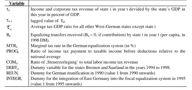
Table 3: list of variables

Variable

τit Income and corporate tax revenue of state i in year t devided by the state´s GDP in

this year in percent of GDP.

τit-1 lagged value of τ_it it

τ Average tax-GDP ratio for all other West-German states except state i

Bit Equalizing transfers received (Bit < 0, if contribution) by state i in year t (per capita, in

1998 DM).

MTRit Marginal tax rate in the German equalization system (in %)

PROGit Ratio of income tax payment to taxable income before deductions relative to the

national average

COMit Ratio of ‚Steuerzerlegung‘ to total labor income tax revenue

DEBTit Dummy variable for the states Bremen and Saarland in the years 1994 to 1998.

REUNt Dummy for German reunification in 1990 (value 1 from 1990 onwards)

INTEGRt Dummy for the integration of East Germany into the fiscal equalization system in 1995

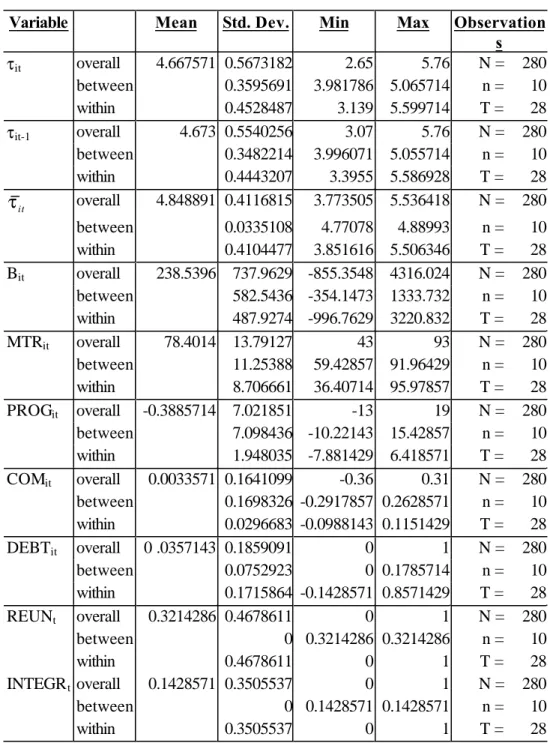
Table 4: Summary statistics

Variable Mean Std. Dev. Min Max Observation

s τit overall 4.667571 0.5673182 2.65 5.76 N = 280 between 0.3595691 3.981786 5.065714 n = 10 within 0.4528487 3.139 5.599714 T = 28 τit-1 overall 4.673 0.5540256 3.07 5.76 N = 280 between 0.3482214 3.996071 5.055714 n = 10 within 0.4443207 3.3955 5.586928 T = 28 it τ overall 4.848891 0.4116815 3.773505 5.536418 N = 280 between 0.0335108 4.77078 4.88993 n = 10 within 0.4104477 3.851616 5.506346 T = 28 Bit overall 238.5396 737.9629 -855.3548 4316.024 N = 280 between 582.5436 -354.1473 1333.732 n = 10 within 487.9274 -996.7629 3220.832 T = 28 MTRit overall 78.4014 13.79127 43 93 N = 280 between 11.25388 59.42857 91.96429 n = 10 within 8.706661 36.40714 95.97857 T = 28 PROGit overall -0.3885714 7.021851 -13 19 N = 280 between 7.098436 -10.22143 15.42857 n = 10 within 1.948035 -7.881429 6.418571 T = 28 COMit overall 0.0033571 0.1641099 -0.36 0.31 N = 280 between 0.1698326 -0.2917857 0.2628571 n = 10 within 0.0296683 -0.0988143 0.1151429 T = 28 DEBTit overall 0 .0357143 0.1859091 0 1 N = 280 between 0.0752923 0 0.1785714 n = 10 within 0.1715864 -0.1428571 0.8571429 T = 28 REUNt overall 0.3214286 0.4678611 0 1 N = 280 between 0 0.3214286 0.3214286 n = 10 within 0.4678611 0 1 T = 28 INTEGRt overall 0.1428571 0.3505537 0 1 N = 280 between 0 0.1428571 0.1428571 n = 10 within 0.3505537 0 1 T = 28

Table 5: Estimation Results (t-values in brackets) τit OLS FE HT HT-dyn. τit-1 ___ ___ ___ 0.3086900 (6.482) * τ_it 0.8712338 (12.791) * 0.9334468 (18.916) * 0.9340806 (13.348) * 0.6640576 (9.580) * Bit -0.0003815 (-8.952) * -0.0002466 (-4.691) * -0.0002748 (-4.380) * -0.0002141 (-4.242) * DEBT 0.8555896 (5.347) * 0.6168470 (4.219) * 0.6813474 (3.606) * 0.5059961 (3.328) * INTEGR -0.1999346 (-2.575) * -0.1420781 (-2.429) * -0.1151997 (-1.416) -0.0824012 (-1.274) REUN -0.0185247 (0.364) 0.0419494 (1.125) 0.0080189 (0.150) -0.0399334 (-0.927) COM 1.5990910 (9.251) * 1.7547600 (3.422) * 1.7542370 (9.560) * 1.2209180 (7.277) * MTR -0.0059301 (-4.279) * -0.0018234 (-1.262) -0.0072833 (-4.813) * -0.0045851 (-3.600) * PROGR 0.0168402 (3.923) * -0.0015591 (-0.240) 0.0220308 (4.621) * 0.0147401 (3.727) * Constant 0.9922344 (2.732) * 0.3214590 (1.160) 0.7671608 (2.034) * 0.4238658 (1.394) R2 0.7667 0.6320 0.7588 0.8489