Public Debt Accumulation and Fiscal Consolidation

(1)

Hitotsubashi University Repository

Title

Public Debt Accumulation and Fiscal Consolidation

Author(s)

Oguro, Kazumasa; Sato, Motohiro

Citation

Issue Date

2011-05

Type

Technical Report

Text Version

publisher

URL

http://hdl.handle.net/10086/19282

(2)

Public Debt Accumulation and Fiscal Consolidation

Kazumasa Oguro Hitotsubashi University Motohiro Sato Hitotsubashi University Abstract

In this paper, we analyze the relationship between interest rates on government bonds (GB) and fiscal consolidation rule by using an overlapping generation model with endogenous and stochastic growth settings.

Our key findings are summarized as follows. First, interest rates of GB may be declining as public debt accumulates relative to private capital, as opposed to the conventional view that buildup of public debt accompanies a rise in interest rates. Second, fiscal consolidation rule plays a key role in determining interest rates in equilibrium. Third, the economy may exhibit discrete changes with interest rates diverging, implying that our observation of relatively low GB interest rates does not assure the continuation of that trend in the future. Fourth, a preventive tax increase to contain public debt at sustainable levels will not gain the political support of existing generations, whose life span is limited. Citizens prefer to shift the ultimate burden of public debt to future generations.

JEL classification: E17; H30; H5; H60; E62; H63

Keywords: Overlapping generation model; interest rate on government bond; fiscal consolidation

rule; default risk

(3)

1. Introduction

Public debt as a percentage of GDP has recently been increasing in developed countries. The gross public debt-to-GDP ratio of Japan is especially high compared to that of other developed countries in 2011. The International Monetary Fund (2009) has estimated that Japan’s gross public debt would reach 277% of GDP by 2016. In such circumstances, interest rates on government bonds (GB) would theoretically rise as a reflection of default risk, as shown by Manganelli and Wolswijk (2009). Codogno et al. (2003), Bernoth et al. (2006), and Akitobi and Stratmann (2008) have also found the existence of spreads that may be interpreted as risk premiums.

On the other hand, interest rates of Japanese Government Bond (JGB) has been lower than that of other developed countries. In addition, we can observe that the interest rates of JGB are currently declining, even though Japanese public debt continues to increase (See Figure 1). A relevant model and mechanism are required to illustrate the seemingly paradoxical confluence of trends. The following possibilities are considered as facets of the mechanism: (1) the reflection of default risk for JGB is weak because 95% of JGBs are held by domestic investors; (2) domestic investors may believe that the Japanese Government will not default on its debt obligations because there are several fiscal reform opportunities (e.g., consumption tax increases) that could help maintain fiscal sustainability; and (3) domestic and foreign investors believe that the interest rate on JGB is low because economic growth under the country’s aging and declining population is expected to be low as well.

Despite these possible motivations, the mechanism for the current interest rate decline remains unclear, and there is no model to explain it. One complication is that GB interest rates also depend on fiscal policy. In particular, fiscal consolidation rule (e.g., tax increases, expenditure cuts, and defaulting on bonds) is important, as governments cannot always roll over public debt to future administrations and generations. Gale and Orszag (2002) and Laubach (2009) have pointed out that the response of GB interest rates on to fiscal policy depends on expectations about the future course of fiscal policy. Perotti (2007) and Favero and Giavazzi (2007) also have found evidence of a change in the relation of macro variables to fiscal policy. This change has been interpreted as evidence of a change in reactions of fiscal policy to stabilization of debt-to-GDP. Uribe (2006) and Juessen et al. (2009) have analyzed government default risk and its reflection on GB interest rates by using a quantitative macroeconomic model. However, Uribe (2006) focuses on external debt with open economy. In the case of external debt, defaulting is considered a deliberate strategic decision of the government that reflects the outcome of an optimization problem (e.g., Eaton and Gersovitz, 1981, or Arellano, 2008). Although Juessen et al. (2009) focus on internal debt using a model with closed

(4)

economy, these theoretical studies never provide examine the potential effects of fiscal consolidation rule on interest rates. Therefore, we provide a macroeconomic model to explain the importance of fiscal consolidation rule; this model clarifies the relationship between decreasing GB interest rates and increasing public debt.

Figure 1 0 0.5 1 1.5 2 2.5 3 3.5 4 4.5 5 0.0 50.0 100.0 150.0 200.0 250.0 1993 1994 1995 1996 1997 1998 1999 2000 2001 2002 2003 2004 2005 2006 2007 2008 2009 2010 % Year General government gross financial

liabilities (percent of GDP) Long-term interest rate

Source: OECD Stats Extracts

In this paper, we consider overlapping generation models with endogenous and stochastic growth settings. The production technology contains spillover associated with private capital and productivity shock. Each generation comprises the representative household that lives for two periods. We account for demographic changes in the economy. Population growth is assumed to be known, but can vary over time. In the young period, the household supplies labor in an elastic manner. Taxes are levied on wages. Part of after-tax wage income is saved. We suppose that there are two types of assets that are tax free. One is private capital and another is GB. The former yields uncertain returns due to the productivity shock of the subsequent period. The latter promises a fixed return, but also a risk of default. As opposed to Juessen, et a (2009)., we consider that default may be partial. In the old period, the household is retired and receives returns on private capital and GBs. Key findings of this paper are summarized as follows: Interest rate of GB may be declining as public debt is accumulated relative to private capital, so the former crowding out the latter as opposed to conventional view that built up of public debt accompanies rise of interest rate. The prospect of future tax increases due to as the fiscal consolidation rule serves to lower expected return on private capital, which in turn decreases interest rates charged on GB through arbitrage. We establish that fiscal consolidation rule plays a key role in determining equilibrium interest rates. In addition, the economy may exhibit discrete changes and diverging interest rates, implying that the declining GB interest rate trend may not continue as public debt further accumulates. We also show that preventive

(5)

tax increases to contain public debt will not gain the political support of existing generations, whose life span is limited. Instead, citizens prefer to shift the ultimate burden of public debt to future generations who cannot currently vote. This confirms the argument that public debt is exploitive of future generations.

The rest of the paper is organized as follows: Section 2 describes the model. In section 3, we consider fiscal consolidation rule and establish equilibrium GB interest rates. Section 4 uses the equilibrium in analysis of comparative statics. We clarify our theoretical argument by simulation in section 5. Section 6 discusses the implications of the results, and Section 7 concludes.

2. Model Setting

2.1 Basic setting

In this paper, we employ a stochastic overlapping generation model. Each generation contains a representative household that lives for two periods. In each period, a single good is produced by labor and capital, but the production is stochastic due to technology shock.

Each period is divided into several stages. At Stage 1, production shock is revealed. The household of the young generation supplies labor at Stage 2. Then output realizes at Stage 3, with wages being paid to the young and return on capital being distributed to the old. The government collects taxes and repays public debt at Stage 4. At Stage 5, the young and the old households consume the former, also saving and choosing a portfolio. Public debt and private capital are carried over to the next period.

To clarify, our analysis follows the two steps. First, we establish intra-period or static equilibrium given public debt and capital carried over from the previous period. We then turn to dynamics. The economic growth is endogenous and stochastic due to productivity shock.

2.2 Production

t

Y

denotes aggregate output at period t that is produced by the representative private firm. The production function of the economy is given as

(1) ₌ε μ α₍ ₎1−α t t t t t t AK k nl Y 4

(6)

where A (>0) is constant, μ > 0 and 0 < α < 1. ε_t denotes productivity shock. For the sake of simplicity, we assume that the shock is distributed according to the distribution function F(εt) over the interval [ε,ε] with Etεt =1. represents private capital that is invested in the previous period, and represents labor supply per worker at period t. Population of generation t is denoted by (t = 1, 2,……). Then represents total labor supply. refers to average capital investment and represents the external effect of capital accumulation. Following the literature on endogenous growth, it may be interpreted as knowledge spillover that serves as a pure public, generating an economy of scale (Romer (1986) ). In the equilibrium, we have .

t k t l t n Lt=ntlt Kt t t K k =

Suppose that production is perfectly competitive. The price of output being normalized to unity, we can write the wage and return on capital as

(2) w_t=(1−α)Y_t/L_t; r_t =αY_t/k_t

As is standard in the literature, market transaction fails to account for the spillover effect in determining the return on capital.

2.3 The household problem

The household’s lifetime utility is assumed to take the following form:

(3) o t t y t t c l c U ₁ / 1 1 ) / 1 1 ( ₊ + + − = δ θ δ

where θ > 0 and δ > 0. denotes the young period of consumption, whereas is the older period. The second term in the first bracket is the disutility of labor supply. It enters in the utility function so that labor supply responds to after-tax wage, abstracting income effect. This simplification follows the literature on optimal income taxation. For instance, see REF. The first bracket term of (3) can be then interpreted as a net gain of the youth period.

y t

c o

t c

The household of generation t supplies labor only after becomes known. However, it is confronted with risks of both productivity shock and government default when making saving decisions. Eq. (3) implies that its preference is neutral to these risks. Given the Cobb Douglas form of the utility function, however, inter-temporal elasticity of substitution turns to be unity. One may find it odd that risk and time preferences are separately defined; our specification deviates from the standard setting that assumes that lifetime utility is additive over periods and over different states of the economy. Inter-temporal elasticity is not tied to the inverse of risk aversion in the present context. Admittedly ad hoc, Eq. (3) helps isolate the household’s portfolio choice between private capital and GB from the decision on total savings, .

t

ε

t

s

(7)

Household budget constraints at the young and the old periods are given by (4.1) cty +st =(1−τt)wtlt ≡ωtlt

(4.2) c~to+1=st

(

qt(1−ζt+1)Rt+1+(1−qt)~rt+1

)

~

where τ_t is wage income tax, ω_t is after tax wages, is the GB’s (one plus) interest rate, and represents the share of the GB in total savings.

t R 1 + t t

q ζ represents the default rate as a value

between zero and unity. The variables with tilde address unknown quantities when saving at period t. is determined at period t with default risk

t

R δt+1; net return on GB is not certain.

1

In the young period, the household decides labor supply and saving and chooses portfolio to maximize returns: t l st t q ] [ ) / 1 1 ( 1 / 1 1 o t t t y t t t E c l c U E + + + − = δ θ η

This is subject to Eq. (4), where the expectation is calculated over ζ_t₊₁ and . The household’s optimization yields the following:

1 + t r (5.1) lt*=ωtδ (5.2) θ + Ψ = 1 * t t s (5.3) 1 1) ~1 ~ 1 ( + + + t − t = t t t E Er R ζ where δ δ δ ω δ ω δ δ δ ω + + + + ≡ ⎟ ⎠ ⎞ ⎜ ⎝ ⎛ + − = + − = Ψ 11/ 1 1 1 1 1 1 / 1 1 t t t t t t l l

By (5.1), wage elasticity of labor is constant at δ. Wage taxation becomes distortive as elasticity increases. Due to the Cobb-Douglas specification, savings is a fixed share of the wage income net of the labor disutility , with income effect and substitution effect offsetting one another as given in (5.2). Finally, (5.3) gives the arbitrage condition between private capital and the GB. Given that the household is risk-neutral, arbitrage leads to the equation of expected return of both assets, which should be intuitive.

t

Ψ

2.4 Market Equilibrium

This subsection considers market equilibrium given fiscal policy. At every period, both labor and capital markets are cleared. Given ε_t and , the equilibrium values of wage and return on private capital at period t are determined by substituting (5.1) into (2) such that

t k

1_{In (4.2), we abstract idiosyncratic risk, including bankruptcy of private capital. This presumes that the household}

can fully diversify such risk and that only aggregate shock will remain. 6

(8)

δ(1−α)/(1+αδ) t t t t A n r

Lastly, we turn to the capital market. Because of the closed economy, household savings must meet demand of private firms and the government. denotes GBs issued at period t and repaid at t + 1.

1 +

t b

2_{Given that total savings at period t is} _{as allocated between} _and _{, the equilibrium} condition is expressed by t ts n kt+1 bt+1 (8)

k

_t₊₁

+

b

_t₊₁

=

n

_t

s

_t* t

(

t tA

)

kt n(1 )/(1 ) ₍₁ ₎₍₁ ₎ (1 )/(1 ) ) 1 )( 1 ( αδ δ αδ α ε τ α δ θ + + + − − − + + =

Manipulating the above establishes the dynamics of private capital accumulation as the following:

(8’) 1 (1 )/(1 )

(

)

(1 )/(1 ) 1 1 ₍₁ ₎₍₁ ₎ ) 1 )( 1 ( 1 δ αδ αδ α ε τ α δ θ + + + − + + + ₋ ₋ + + = ⎟⎟ ⎠ ⎞ ⎜⎜ ⎝ ⎛ + t t t t t t t n _A k k k b

Now consider growth rate. This economy grows at the rate of χ_t₊₁ that is stochastic and defined as (9) t t t t t t t t t t t _k k n n Y Y 1 ) 1 /( ) 1 ( 1 ) 1 /( ) 1 ( 1 ) 1 /( ) 1 ( 1 1 1 ~ 1 ~ 1 ~ ~ + + − + + + + + − + + + ⎟⎟ ⎠ ⎞ ⎜⎜ ⎝ ⎛ ⎟⎟ ⎠ ⎞ ⎜⎜ ⎝ ⎛ ⎟⎟ ⎠ ⎞ ⎜⎜ ⎝ ⎛ − − = ≡ αδ α αδ δ αδ α δ ε ε τ τ χ

As opposed to the growth model with agents of infinite life, the OLG may exhibit dynamic inefficiency, in which growth rate becomes lower than interest rate. The following lemma yields the condition that the economy remains dynamically efficient:

2_{We consider only a single period bond, and thus we abstract issues of bond maturity composition.}

(9)

Lemma 1: The economy is dynamic efficient, or χt+1≤rt+1 if _θ _δ α α _≤ + + − ) 1 )( 1 ( 1

Proof of this is shown in Appendix A. Throughout the paper, we assume that the above inequality holds.

2.5 Government budget

The government raises revenue by issuing GB and taxing wage income. It then spends this on debt repayment and public expenditure, the latter being denoted by . is assumed to not contribute to production (1) or directly enter into household utility (3). This assumption is motivated to simplify our analysis, but may be plausible when government spending comprises political rents or pork diverted to special interest groups. The funding flow of the government budget at period t is written as t G Gt (10) bt+1=Rtbt−{Tt−Gt} t t t t t t wL Y T

where =

τ

=(1−

α

)

τ

and is given in (7’). For the latter, the following lemma

establishes the revenue-maximizing tax rate that determines the upper bounds for tax rates in the case of fiscal consolidation:

t

Y

Lemma 2: Tax revenue is maximized at

δ αδ τ + + = 1 1 Max

At this point, we distinguish fiscal rule between pre-fiscal consolidation and fiscal consolidation

regimes. This is denoted by , which contains tax rate , government expenditure

ratio } , , { t t t t ≡ τ λ ζ Ω τ_t t

λ , and default rate , and may be state-contingent for consolidation regimes. Fiscal rules are assumed to be public information, implying that these rules are incorporated in the pricing of GB, as discussed below. The present model does not suppose optimization behavior of the government in the pursuit of social welfare. We instead take the pragmatic view that government policy is largely politically constrained, as opposed to being designed based on economic rationale.

t

ζ

Let _Ω0_≡{_τ,_λ,_ζ}, with _ζ ₌₀_{. In the pre-consolidation regime, the government taxes wage income} at the rate of τt =τ and spends a given portion of potential output, λt =λ, that calculates at the mean of

t Y t

ε ; that is, εt=1 and τt =τ, such that Gt =λYt, where

(11) Yt

(

} , , { 0_≡ _τ _λ_ζ Ω 0 ) , , ( <

Δτ λ εt for most of εt. The public debt may reached a level at which the status quo fiscal rule cannot be sustained. We do not suppose that the government undertakes precautionary measures to prevent such circumstances. Political economy considerations on such measure will be discussed later.

Given the OLG setting, a capital market may not work to discipline government financing, because the finite-life household may not be concerned with long run fiscal sustainability. Unless it is certain that ζ_t₊₁=1 with risk-neutral preference and that (5.3) holds, a household will purchase GB, with the default risk perceived as being compensated by a higher ex ante promised interest rate.

In the present context, therefore, the government can access credit insofar as the GB level does not exceed domestic savings with the interest rate fulfilling (5.3). Suppose, however, that the economy reaches , that is, the domestic savings at period t + 1 is fully absorbed by government borrowing, given that the economy is closed and no private investment can take place, which implies

1 1 2 + + + = t t t n s b 9

(11)

that there is no production in the subsequent period, or Yt+2=0 for all εt+2. Once this occurs, the

government can find no resource for repayment. It then has to default on the debt so that ζ_t₊₂=1 is certain, and therefore, there will be no return on GB.3 This in turn implies that the households cease to lend to the government. The government is then forced to undertake fiscal consolidation without further borrowing. This entails tax increases, expenditure cuts, and further defaulting on GB.

Lemma 3: Full default is inevitable at period t + 1 irrespective of εt+2 when bt+2=nt+1st+1.

With bt₊₂=nt₊₁st₊₁ or kt+2=0, we have bt+2/kt+2=∞at period t+1. The literature of fiscal

sustainability discusses the transversality condition of the present value of the public debt in the infinite future. Indeed, Juessen et al. (2009), using infinitely living agents, considers that the government is forced to default on its debt once the condition fails to hold. In the OLG setting, however, the household is willing to purchase GB in its young period, when debt repayment occurs in the next period or the consolidation risk is compensated with a higher GB interest rate. To state it differently, the transversality condition does not define government default in the present model. See Appendix B.

3.2 The threshold

Inserting bt+2/kt+2=∞ 1 + t

into (13) and manipulating it yields the following condition of the threshold level of ε , below which regime change occurs:

(14)

(

)

( )

_⎟⎟ ⎠ ⎞ ⎜⎜ ⎝ ⎛ ⎟ ⎠ ⎞ −α λ 1 ⎜ ⎝ ⎛ + ε τ ˆ_t − − + − − = − + + + + + + + + α αδ α τ δ αδ ε _τ δ αδ 1 1 1 ( ˆ ( ) 1 ( 1 1 (1 )/(1 ) ) ) 1 /( ) 1 ( ) 1 /( ) 1 ( 1 1 1 t t t t t n A k b R + + + + + δ θ αδ δ ) 1 )( )(1 )/(1 1

This defines the threshold εˆ_t₊₁ implicitly as the function of the interest rate charged on , as

well as debt-to-capital ratio and demography: where .

1 + t b ) 1 + ) , 1 1 + + t t Z R ( ˆ ˆ_t₊₁=ε_t₊₁ ε Zt+1=(bt+1/kt+1,nt 4_With and , 1 + t

R bt+1/kt+1 εˆt+1 increases such that fiscal consolidation is more likely to be in place,

whereas it is lowered with n_t₊₁.

Lemma 4: Fiscal consolidation must occur at period t + 1 when εt+1≤εˆt+1

Fiscal consolidation involves tax increases, expenditure cuts, and defaulting on GB. The state of the economy at period t+1 is denoted by Ξt+1=(εt+1,bt+1/kt+1,nt). The fiscal rule is then expressed as

, with , which contains

) ( 1 1 + + ≡ΩΞ Ωt t bt+2=0

3_{On the other hand, return on private capital remains positive, with the revenue maximizing tax rate being bounded}

by less than 100%.

4_{We let}_ε ₌_ε

+1

ˆ_t when the LHS exceeds the RHS at εˆ_t₊₁=ε. Note that the fact that consolidation is inevitable

with εˆt+1=ε_{does not mean full default, that is,}ξt+1=1, given that bt+1/kt+1 remains at a finite level.

(12)

τ τ

τ

τ ≤ t+1= (Ξt+1)≤ ,λ≥λt+1=λ(Ξt+1) 0≤ζt+1=ζ(Ξt+1)≤1

where the default rate fulfills5

(15) (1 )

(

(1 )

)

(1 )/(1 ) ( ₁, ₁, ₁) 1 ) 1 /( ) 1 ( 1 1 1 1 +− + + + + + + + + + + = − Δ − _t _t _t _t t t t t _k A n b R α τ λ ε ζ δ αδ α αδ

The government cannot fully meet its obligation but repays its outstanding debt as much as possible out of the primary surplus, as illustrated in (15). Under the consolidation rule, either tax rate, expenditure ratio, or default rate deviates from the initial levels. The fiscal rule can take a general form, but may be plausibly levied according to the following restrictions:

(Assumption2) 0 ) / ( ) (i ∂τt+1 ∂bt+1 kt+1 ≥ (ii)∂ζt+1 ∂(bt+1/kt+1)≥0 (iii)∂λt+1 ∂(bt+1/kt+1)≤0

In the simulation of section 5, we specify fiscal consolidation rule. Note that it takes only one period to restructure government finance. Given that no GB is issued, the economy will return to the initial regime in the next period without debt liability being carried over.

3.3 Interest rate

Let us turn to GB interest rate , which is settled at period t, accounting for fiscal consolidation in the event of . Recall the arbitrage condition (5.3), which equates return on GB and capital in the expected term. Manipulating it with the use of (6.2) and (15) establishes the following:

1 + t R 1 1 ˆ+ + ≤ t t ε ε (16)

₍

₎

⎭ ⎬ ⎫ Δ − ⎩ ⎨ ⎧ _Φ − − = −

∫

+ + + + + + + + + + + + − + + + ) ~ ( ) ~ , ~ , ~ ( ) , ˆ ( 1 ) 1 ( )) ˆ ( 1 ( 1 ˆ 1 1 1 1 1 1 1 1 ) 1 /( ) 1 ( ) 1 /( ) 1 ( 1 1 1 t t t t t t t t t t t t dF b k A n R F ε αδ δ αδ α _ε _τ _τ _λ _ε _ε α α α ε 　　　　 where

( )

_∫

( )

∫

+ + − + + + + + + + + + + − + + + − + − = Φ 1 ) 1 /( ) 1 ( 1 ˆ 1 ) 1 /( ) 1 ( 1 ˆ 1 ) 1 /( ) 1 ( 1 ) 1 /( ) 1 ( 1 1 1 ) ( ) 1 ( ) ( ) 1 ( ) , ˆ ( t t t t t t t t t dF dF ε αδ δ ε _δ _α _αδ _δ _αδ ε ε τ ε ε τ τ ε αδ α δ

and τ_t₊₁ of Φ(εˆt+1,τt+1) means the vector of τt+1

Note that Φ(εˆt+1,τt+1) reflects the expected return on private capital.

6_{We can clearly see that it is} non-increasing with the threshold level, given that τ≤τt₊₁. This represents the perverse effect of wage tax increases under fiscal consolidation that discourage labor supply and in turn lower the productivity of private capital.

5_{The consolidation rule can be interpreted in a reduced form that incorporates the dependency of the equilibrium}

values of R_t₊₁_andεˆ_t₊₁_on Zt+1=(bt+1/kt+1,nt). 6 ₍ ₎ ₍ ₍₁ ₎₎ ₍_ˆ _, ₎ 1 1 1 ) 1 /( ) 1 ( ) 1 /( ) 1 ( 1 1 + − + + + + + + t = ₋ t − Φ t t t r n A E α ε τ α α α αδ δ αδ 11

(13)

(16) yields the GB interest rate as a function of the threshold, the debt-to-capital ratio, and the population: Rt+1=Rt+1(εˆt+1,Zt+1). The effect of εˆt+1 is described in the following lemma:

Lemma 5:

Denoting τˆ_t₊₁=τ_t₊₁(εˆ_t₊₁,Z_t₊₁)and ζˆt₊₁=ζˆt₊₁(εˆt₊₁,Zt₊₁) whereZt+1=(bt+1/kt+1,nt), we have

(

)

(1 )/(1 )

₍

(1 )/(1 )

₎

1 ) 1 /( ) 1 ( ) 1 /( ) 1 ( 1 1 1 1 1 1 ( ˆ 1 ) 1 ( ˆ 0 ˆ αδ α αδ δ αδ δ αδ α _ε _τ₎δ(1α)/(1αδ) ₍₁ _τ_ˆ₎δ α α α ζ ε + − + + + + + + − + + + + + − − − < > ⇔ < > ∂ ∂ t t t t t t A n R R 1 + t R

ε

ˆ_t₊₁ ˆ / 1 1 + − ₋ ₋

The proof is shown in Appendix C. This lemma implies that the interest rate is increasing (resp. decreasing) in when fiscal consolidation entails no tax increase (resp. no default) and thus revenue loss is made up for by defaulting on outstanding debt (resp. by raising tax) at the threshold level. It may be counterintuitive that may be lowered as increases. To see the point, note that in the present model, fiscal consolidation involves both the default and the tax increase. The former adds the risk premium of GB relative to private capital, thereby raising its interest rate. The latter, on the other hand, reduces the return on private capital, which works to lower the GB interest rate through arbitrage. We then have the case of

1

ˆ_t₊

ε

0

<

∂Rt+ ∂εt+ when tax increases dominate the

default risk.

Consider the increase of . is increasing with it, since the productivity of private capital is enhanced as labor supply is enhanced. On the other hand, the impact of the debt-to-capital ratio is

ambiguous as well. , directly appearing in (16), serves to raise , whereas by

Assumption 2, the induced tax increase under consolidation works in the opposite direction. That is, 1 + t n R_t₊₁ 1 1/ + + t t b k R_t₊₁ 0 ) / ( 1 1 1 ∂ ≥ ∂τ_t₊ b_t₊ k_t₊ .

To clarify our analysis, it will be of help to consider extreme consolidation rules as follows:

No Tax Increase: Let τ(Ξt+1)=τ _{for all}εt+1, such that there is no need for a tax increase.

Consolidation entails defaulting on outstanding debt as well as cutting government expenses. The default rate fulfills

(15’) (1 ( ))

(

)

(1 )/(1 ) ( , ( ₁), ₁) 1 ) 1 ( 1 1 1 1 +− + + + + + + + + = − Δ Ξ Ξ − _t _t _t t t t t _k A n b R α τ λ ε ζ α αδ ) ( 1 1 + + =Ω Ξ ΩD D _t t 1 1 + + = t t R R 1 ( δ)/(1+αδ

represents such fiscal consolidation. According to Lemma 5, the function of

1 ˆ_t₊ ε ) , ˆ

(εt+1 Zt+1 _{should be upward with respect to} .

(14)

No Default: Suppose instead that no default is allowed, or ζt+1=0 for all , but the outstanding

debt must be fully repaid through tax increases and expenditure cuts, with 1 + t ε ) ( 1 1 + + = Ξt t τ τ being

implicitly determined by (15) withζt+1=ζ(Ξt+1)_{= 0. Let} denote fiscal rule. Then, (16) reduces to ) (Ξt+1 ND 1 + =Ω ΩND t

(

)

(ˆ , t+1) 1 ) 1 ( 1 ) 1 /( ) 1 ( ) 1 /( ) 1 ( 1 + + + + − + − ₋ Φ t t A n ε α α α δ αδ αδ α 1 ˆ_t₊ 1 + = t R τ (16’)

which is decreasing with ε .7 is also decreasing in the debt-to-capital ratio, given that the RHS of (16) decreases as 1 + t R is raised.8 ) ( 1 1 + + = Ξt t τ τ

3.4 Interaction

There exists interaction between the threshold of the fiscal consolidation εˆ_t₊₁ and the GB interest rate , defined by (14) and (16) respectively. Solving these equations yields their equilibrium values. Note that these are assessed from period t or ex ante perspective when is not known and fiscal consolidation is not yet in place.

1 + t R ) ( 1 1 + + =ΩΞ Ωt t 1 + t ε * 1 + t R * 1 ˆ_t₊ ε 1 1/ + + t t k

Proposition 1: Denote by and the equilibrium levels of the GB interest rate and the

threshold of fiscal consolidation conditional upon b and the consolidation rule

. These are given as solutions to the following equations:

( )

(

)

(

)

_⎟⎟ ⎠ ⎞ ⎜⎜ ⎝ ⎛ ⎟ ⎠ ⎞ ⎜ ⎝ ⎛ − − + − = + + + + + + + + − + + + _α λ ε τ τ δ θ ε τ αδ δ αδ δ αδ αδ α 1 ˆ 1 1 ) 1 )( 1 ( ) ˆ ( ) 1 1 (1 )/(1 ) ) 1 /( ) 1 ( 1 ) 1 /( ) 1 /( ) 1 ( 1 1 1 t t t t t t n k b R − + + −α (1 A(1+δ)

(

)

⎭ ⎬ ⎫ Δ − ⎩ ⎨ ⎧ _Φ _Τ − − = − (ˆ₊ 1 ( F εt1

∫

+ + + + + + + + + + + + − + + ) ~ ( ) ~ , ~ , ~ ( ) , ˆ ( 1 ) 1 ( )) 1 ˆ 1 1 1 1 1 1 1 1 ) 1 /( ) 1 ( ) 1 /( ) 1 ( 1 1 t t t t t t t t t t t dF b k A n R ε αδ δ αδ α _ε _τ _λ _ε _ε α α α 　　

In the above proposition, we do not preclude the case that there arise multiple equilibria, with the two equations intersecting more than twice or with the equilibrium diverging, that is, * reaching

1 ˆ_t₊ ε as illustrated below. ε Corollary to Proposition 1:

7_{The sufficient condition for} ₍ ₎_{to exist is given by:}

1 1 + + =Ω Ξ ΩtND ND t Δ(τ,0,ε)≥

( )

_⎟⎟ ⎠ ⎞ ⎜⎜ ⎝ ⎛ ⎟ ⎠ ⎞ ⎜ ⎝ τ ⎛ − − − + + + − + + + + + + α λ ε τ δ θ ε τ δ αδ δ αδ δ αδ 1 1 1 ) 1 )( 1 ( ) ( 1 (1 )/(1 ) ) 1 /( ) 1 ( ) 1 /( ) 1 (

8_{One may note that government financing can be regarded as sustainable in the present context even for}

1 1 ˆ+ + ≤ t

t ε

ε

without default. We interpret fiscal sustainability in a slightly strict way, in that it refers to a circumstance in which status quo fiscal policy including taxation and expenditure can be sustained.

(15)

In the corner equilibrium with ε =ˆ*t+1 ε, we can define the GB interest rate Rt*+1 if there exists a

consolidation ruleΩt+1 =Ω(Ξt+1)that fulfills9

) ~ ( ) ~ ), , ~ ( ), , ~ ( ( )) ( , ( 1 1 1 1 1 1 1 1 1 1

∫

+ + + + + + + + + = Δ Ξ Τ Φ − ε ε ε ε λ ε τ ε α α t t t t t t t t t _b Z Z dF k

with no default at ε_t₊₁ =ε _{so that}

(

(1 )

)

(1 )/(1 ) ( ( , ₁), ( , ₁), ) 1 ) 1 /( ) 1 ( 1 1 * 1 α α αδ τ ε λ ε ε αδ δ + + + − + + + + + + = − t Δ t t t t t A n Z Z k b R where 1 * 1 + + > t t R R ( 10_and

are the solution to

1 + t R( = ˆt₊₁(Rt₊₁,Zt₊₁) ( ε ε _.

In the corollary, the default rate is set to zero at εt+1=ε. The consolidation rule at the corner

equilibrium may differ from the one applied to the interior one. The presumption is that the representative household forecasts Ωt+1 when it anticipatesε =ˆ*t+1 ε. Also note that 1

*

1 +

+ > t t R

R ( _{is to}

assure that (14) yields εˆt+1=ε, taking as given Rt*+1

) , ( ˆ ˆt₊₁= t₊₁ Rt₊₁ Zt₊₁ .

4. Comparative Statics

4.1 Debt accumulation

Regarding comparative statics, totally differentiating the equation (14) of threshold ) , ˆ ( 1 1 1 1 + + + + ε

ε and the equation (16) of the GB interest rateRt =Rt εt Zt establishes

(17) 1 1 1 1 1 1 1 1 * 1 1 1 /) ( / ˆ ) ( ) / ( / ˆ ˆ ) ( / ˆ + + + + + + + + + + + + + ⎥ ⎥ ⎥ ⎤ ⎢ ⎢ ⎢ ⎡ ∂ ∂ − ∂ ∂ + ⎟⎟ ⎠ ⎞ ⎜⎜ ⎝ ⎛ ⎥ ⎥ ⎥ ⎤ ⎢ ⎢ ⎢ ⎡ + ∂ ∂ = ⎟ ⎟ ⎟ ⎟ ⎞ ⎜ ⎜ ⎜ ⎜ ⎛ ⎥ ⎥ ⎥ ⎤ ⎢ − ∂ ∂ − t t t t t t t t t t t t t dn n R n k b d k b d R ε ε ε ε ₁ 1 1 ⎢ ⎢ ⎡ 1 1 1 * 1 1 1/ ˆ+ 1 + + / ( + / +) ( ) + ⎥⎦⎝⎜ ⎠⎟ ⎢⎣∂ ∂ ⎥⎦ ⎢⎣ + ⎥⎦ ⎢ ⎣−∂Rt ∂εt dRt Rt bt kt ) / ˆ )( ˆ / ( 1− ∂ +1 ∂ +1 ∂ +1 ∂ +1 ≡ Rt t t Rt H

Meanwhile, we focus on the interior and stable equilibrium where the equilibrium interest rate is

finite, with ε ε _{> 0. Then we obtain the following proposition in the}

case of no demographic change.

9_{The sufficient (and strict) condition for such fiscal rule to be feasible is:}

( , ) ( ,0,~ ) (~ ) 1 1 1 1 1

∫

+ + + + _Δ < Φ − ε

ε

τ

ε

α

t t Max t t Max _b dF k

Given that the LHS is declining with the wage tax rate.

10_{This inequality is re-written as:}

Δ(τ(ε,Zt+1),λ(ε,Zt+1),ε)

( )

⎟⎟ ⎠ ⎞ ⎜⎜ ⎝ ⎛ ⎟ ⎠ ⎞ ⎜ ⎝ ⎛ − − − + + + − > + + + + + + α λ ε τ τ δ θ ε τ δ αδ δ αδ δ αδ 1 1 1 ) 1 )( 1 ( ) ( 1 (1 )/(1 ) (1 )/(1 ) (1 )/(1 ) 14

(16)

Proposition 2: The debt-to-capital ratio (i) * is increasing if 1 ˆ_t₊ ε ∂Rt+1/∂(bt+1/kt+1)≥0 0 / 1 1 >

(ii) * is increasing if and

1 + t R ∂Rt+ ∂εt+ ∂Rt+1/∂(bt+1/kt+1)≥0 0 / 1 1

(iii) * is decreasing if and

1 + t R ∂Rt+ ∂εt+ < ∂Rt+1/∂(bt+1/kt+1)≤0 0 / ₁ 1 ∂ > ∂R_t₊ ε_t₊ 0 / ( / 1 1 ∂ ∂Rt+ bt+ ( ˆ ˆt₊₁= t₊₁ Rt₊₁

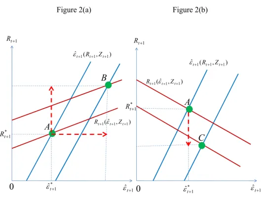
Figure 2 depicts possible scenarios. Figure 2(a) gives the case of and

. The initial equilibrium is located at point A. Increasing the debt-to-capital

ratio moves ,Zt+1) ) 1 ≥ + t k rightward and Rt+1=Rt+1(ˆt+1,Zt+1)

ε ε ε upward. The intersection of the

two functions is then shifted up and right such that both the interest rate and the threshold are raised. In Figure 2(b), Rt+1=Rt+1(εˆt+1,Zt+1) is sloped downward. The initial equilibrium is again given by point A. εˆt+1=εˆt+1(Rt+1,Zt+1) moves in the same way as Figure 2(a), with . Suppose

. The threshold is raised, moving the new equilibrium to point B. The change in interest rate is not certain. Let

1 1/ + + t t k b 0 ) / ( / 1 1 1 ∂ > ∂Rt+ bt+ kt+ 0 ) 1 / ( / 1 1 ∂ ≤

∂Rt+ bt+ kt+ . Rt*+1 is then lowered to point C, whereas

change in * is ambiguous.

1

ˆ_t₊

ε

Figure 2(a) Figure 2(b)

1 ˆ_t₊ ε εˆt+1 1 + t R 1 + t R

0 ₀

) , ˆ ( 1 1 1 + + + t t t Z R ε ) , ˆ ( 1 1 1 + + + t t t Z R ε ) , ( ˆ_t₊₁ R_t₊₁ Z_t₊₁ ε ) , ( ˆ_t₊₁ R_t₊₁ Z_t₊₁ ε

A

B

C

* 1 + t R * 1 ˆ_t₊ ε * 1 ˆ_t₊ ε * 1 + t R

The upshot is that we have the circumstance that decreases with debt being accumulating relative to private capital as depicted in Figure 2(b). This is likely when fiscal consolidation rule includes large tax increases while keeping the default rate low at most of

* 1 + t R 1 + t ε , such as

as discussed earlier. (In contrast, Figure 2(a) implies that the default risk is ) ( 1 1 + + =Ω Ξ ΩND ND _t t 15

(17)

significant in the fiscal rule.)

It is often addressed that as consequence of crowding out private investment, the buildup of public debt leads to surges in interest rates. The presumption of such an argument is diminishing marginal returns on investment. Decreased private capital then enhances its productivity on margin, which in turn raises market interest rate. The endogenous growth setting, however, does not translate the crowding out into such increases of the marginal product of , as it is fixed depending upon the wage tax rate and other economic environment. Rather, expectation of future tax increases reduces the expected return on private capital, which is in turn reflected in lower levels of . To state it differently, lower signals a cautionary view of future government financing in the present context. 1 + t k 1 + t R 1 + t R * 1 + t R * t R 1 1/ + + t t k b 0 / ₁ 1 ∂ > ∂R_t₊ ε_t₊ Ω(Ξ_t₊₁) 0 ) / ( / ₁ ₁ 1 ∂ ≥ ∂R_t₊ b_t₊ k_t₊ R_t₊₁(εˆ_t₊₁,Z_t₊₁) 3 2_<₍_b_/_k₎ ₍_b_/_k₎1 1 + t k

At this point, it is worth addressing that consolidation rule plays a key role in determining equilibrium. If consolidation is done mostly by defaulting the public debt as in the extreme, the case of Figure 2(a) becomes likely, raising as the public finance deteriorates. The contrasting trend shown in Figure 2(b) is observed when consolidation includes a significant tax increase while respecting the debt obligation. It can be perceivable that is lower in the latter fiscal rule than the former, given . The different fiscal rules are compared in the simulation as well. ) ( 1 1 + + =Ω Ξ ΩD D _t t 1 +

4.2 Discrete Change

In Figure 2, we assume a unique and interior solution to equations (14) and (16). However, we may have multiple or corner equilibria. Figure 3 illustrates such to be the case, assuming

given the consolidation rule applied to the interior equilibrium. Also,

suppose such that the curve of moves upward along with

the debt-to-capital ratio.

The figure depicts three different levels of the ratio with . At , the

GB interest rate and the threshold functions intersect only once at point A that yields unique equilibrium. For the middle level of the ratio, the two functions turn to cross twice at points B and C. Point B gives stable equilibrium, whereas C is unstable. In the case of multiple equilibria, outcome depends upon belief of the household who purchases GB.

1 ₍ _/ ₎

) /

(b k < b k

11_{Note that further increasing}

1/ +

t b

11_{In a more general context in which households of one generation are heterogeneous, some coordination of beliefs}

is needed to determine which equilibrium is achieved. 16

(18)

shifts the two curves so that points B and C come too close. They touch one another at D in the case of , beyond which the interior solution disappears. This implies that the economy moving along the stable interior equilibrium may exhibit a discrete change to the corner solution with higher interest rates and threshold. Thus, the observation that GB interest rate has remained relatively low does not assure that the same trend continues in the future as public debt accumulates.

( )

_b_/_k 3 Figure 3 1 ˆ_t₊

ε

1 + t R 0 D 1 ) / (b k ( •) = + + +1 t1 ˆt 1, t R R ε ε * 1 ˆt+ ε * 1 + t R B C

(

•

)

= + + + ˆ , ˆ_t ₁ ε_t ₁ R_t ₁ ε A 1 ) / (b k 2 ) / (b k 2 ) / (b k 3 ) / (b k 3 ) / (b k

In the figures, we address the circumstances in which the buildup of public debt might lead to lower GB interest rates owing to the prospect of future tax increases relating to fiscal consolidation, and in which there might thus be a sudden rise of interest rates from relatively stable and low rates to extreme levels, thus increasing the fiscal consolidation risk. We confirm these scenarios by simulation in section 5.

4.3 Demographic Impact

Lastly, we examine the effects of demographic change. Note that in the endogenous growth model, the population or labor force is a key driving force to enhance productivity. With population size lowered, productivity decreases and thus the expected return on capital is diminished, which in turn works to reduce . The threshold of the regime _{switch is increased, on the other hand,} because the primary surplus is lowered. These interacting, the net impact is as stated in the following proposition: 1 + t R εˆ_t₊₁ 17

(19)

Proposition 3: Consider reduction in nt+1. Then (i) * decreases if 1 + t R ∂Rt+1/∂εt+1<0

(ii) * is enhanced if is increasing

1 ˆ_t₊ ε * 1 + t R * 1 + t R * 1 ˆ_t₊ ε

In general, the equilibrium effects of the demographic change on and are ambiguous. In section 5, we conduct a simulation to compare the scenarios of different demographic changes.

4.4 Debt accumulation

In the previous section, _{was taken as fixed and the equilibrium was established as} conditional upon it. We now consider accumulation of public debt. It is stochastic as it relies on realization of the productivity shock. Combining (8’) and (13) and advancing the period by one, we obtain the transition process of the debt-to-capital ratio as follows:

1 1/ + + t t k b (17)

(

)

(

)

( )

_⎪⎭⎬ ⎪⎩ ⎨ ⎪⎫ ⎪ ⎟ ⎟ ⎠ ⎞ ⎜ ⎜ ⎝ ⎛ − − + − − × − − + + = + + + + + + + + − + + − + + + + + + + ) 1 ( ~ ~ ) 1 )( 1 ( / ˆ ) 1 )( 1 ( ) 1 )( 1 ( / 1 / ) 1 /( ) 1 ( 1 ) 1 /( ) 1 ( 1 ) 1 /( ) 1 ( 1 ) 1 /( ) 1 ( 1 1 * 1 2 2 2 2 α τ ε λ ε τ α τ α δ θ αδ δ αδ δ αδ α αδ α δ t t t t t t t t t t A n k b R k b k b 1 ⎧ ~

where εt+ addresses that its value is uncertain at period t.

The immediately higher is transited to a higher in the next period given

accounting for the dependency of on b . According to Proposition 2, this implies that the risk of fiscal consolidation at period t + 1 is raised with the current debt-to-capital ratio if

. 1 1/ + + t t k b bt+2/kt+2 εt+1 * 1 + t R t+1/kt+1 0 ) / ( / 1 1 1 ∂ ≥ ∂Rt+ bt+ kt+ 1 + t n 1 1/ + + t t k ) , / , ( ˆ * 1 1 1 t t Rt b k n t+ =ε+ + ε εt+1 0 1 1/k (b/k) bt+ t+ = 1 1 1/kt+ =(b/k) + εt M

Figure 4 depicts the shape of the transition function (17) with constant _{at n. It shows three} levels of : low, middle, and high. Note that a smaller value of shifts (17) upward. Also note

that the curve approaches infinity if b _{goes to the critical level such that}

; that is, becomes coincident with the threshold of fiscal consolidation. Suppose that . By (17), the debt-to-capital ratio carried over to the next period is

given by b , being located at point E if . In the figure, we have

t ε ε_t₊₁ t +1=ε

( )

(

)

_εM L t ε ε =+1 H ε = 1 bt+2/kt+2 t R*+1 t L _ε _b _k ε < ₊ 1 < 1 , / ˆ 0 2 = + t b

, which implies that there arises a regime change at period t+1 if ,

whereas government financing is sustainable when . Figure 4 shows that

approaches infinity at without consolidation. In the event , no public debt, that is, , is issued under the consolidation rule, and thus, the economy moves back to its origin. On

t ε+ L t ε ε =+1 εt+1=εL 18

(20)

the other hand, the ratio is lowered to 2_{or point F when} . 2 2/k (b/k) bt+ t+ = ε =t+1 εH Figure 4 1 1/ + + t t k b 2 2/ + + t t k b

0

1 L ε _εH M ε ( )_b_/_k0 ( )1 /k b ( )_b_/_k2 E F L ε = 2 M t ε ε+2= t ε+ t ε+ H ε = 2

5. Simulation

5.1 Specification

This section aims to conduct a simulation of the comparative statics developed in section 3. To be specific, we examine the theoretical hypotheses that public debt accumulation may lead to lower interest rates and that the equilibrium interest rate may exhibit a discrete change from relatively low to an extreme high level. In addition, we confirm whether the equilibrium in the pre-consolidation regime is affected by fiscal consolidation rule and demographic change. Moreover, we calculate the threshold at which consolidation occurs given at period t. Needless to say, our quantitative analysis does not intend to replicate any practice of economy. Rather, it is to supplement our theoretical model, resolving ambiguity of its results and clarifying its policy implications.

t t k

b /

The parameters are specified in Table 1. distributes over [0.5 1.5] according to the inverse U-shaped density function with mean of one. We set the tax rate at a relatively low 10%. We set the expenditure rate at 10% of potential output as well. This implies that primary deficit is likely to result unless is larger than mean of one, so there exists the possibility that public debt is accumulated, with consolidation risk thus being enhanced. Fiscal consolidation rule commands the

t ε

(21)

expenditure to be cut in half to . The wage tax rate under consolidation is increasing in , whereas it increases with as imposed by Assumption 2. This is specified in Table 1. Consolidation relies on more tax increases for large debt to capital ratio, whereas the default rate is raised when 05 . 0 1= + t λ 1 + t ε bt+1/kt+1 1 + t

ε is small and the economy is therefore depressed. Such presumption should be plausible.

The parameter g in the tax function refers to the extent of the required tax increase. The simulation set three values of g (0.5, 0.75, and 1.0). Higher g implies a larger tax increase in the consolidation, which in turn implies a lower default rate that is defined as residual by (15): the tax function above is constrained so that _{takes interior value. By comparing results of different levels of g,} we can assess the effect of fiscal rule on and as well as the transition of the debt-to-capital ratio. To examine the demographic change, we consider the case that the population remains constant over time and also the case that it is declining. In the latter, we assume that it annually

decreases by 0.3%. Taking one period to stand for 30 years, we let . Distinct by

the parameter g and the demography, four scenarios are presented as summarized in Table 2. Scenario 1 is taken as a benchmark in the following table.

1 + t ξ 1 + 1 + t ξ * 1 ˆ_t₊ ε t t n n 30 1=(1−0.03) + * t R Table 1: Parameters δ 0.5 α 0.3 θ 1.333 Ａ 7.0 } ,ζ λ Ω0_≡{_τ, _τ_{= 0.1}_λ_{= 0.1} ) (Ξ+1 Ωt+1≡Ω t ⎟⎟ ⎠ ⎞ ⎜⎜ ⎝ ⎛ + × = + + + 1 1 1 8 . 3 , ( t t t Max _k b g Min τ τ ε ε τ 1 . 0 ( + +1 1 1,bt /kt ) ) / , 1 1 1 + t + + + bt kt t ε λ = Table 2: Scenarios Scenario 1 (Benchmark) g = 0.75 1 1= + t n Scenario 2 g = 0.5 Scenario 3 g = 1.0 Scenario 4 g = 0.75 30 1= (1−0.003) + t t n n

5.2 Results

In simulation, we focus only on the interior equilibrium. The GB interest rates for different scenarios 20

(22)

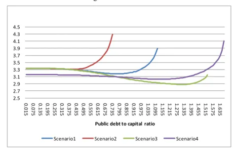
are shown in Figure 5, where is treated parametrically taken on horizontal axis. In all scenarios, there exists a range in which _{exhibits downward sloping, confirming our theoretical} hypothesis. Take the benchmark scenario (Scenario 1). The interest rate is initially declining, with

. Its moderate downward trend continues until =0.78, where takes the

minimum value. The slope is then reversed, further increasing the debt-to-capital ratio and rapidly raising the interest rate. At =1.11, the stable interior level of disappears, diverging to the corner equilibrium (which is not explicitly treated here). This is consistent with the illustration of Figure 4. 1 1/ + + t t k b 1 /kt+ * 1 + t R 1 1/ + + t t k b bt+1/kt+1 Rt*+1 1 + t b * 1 + t R 1 1/ + + t t k b bt+1/kt+1 1= + t

The benchmark scenario is compared with Scenario 2 and 3 to assess impacts of the tax increase. in Scenario 2 barely differs from the benchmark for low levels of . After ₌ 0.3, however, the former begins to exceed the latter, and the difference between them widens quickly. Once the ratio goes beyond 0.735, Scenario 2 loses its interior equilibrium, whereas it remains in the benchmark scenario. In the former, with g = 0.5, the tax increase is less significant than the latter when fiscal consolidation is implemented. Given that both scenarios impose

* 1 + t R 05 . 0 λ _{in the}

event of the consolidation, this implies that Scenario 2 experiences a higher default rate and consequently adds a risk premium to GB. Now consider Scenario 3, with g = 1. Again, its interest rate moves about the same as the benchmark when the public debt-to-capital ratio is not high. For >0.5, the disparity turns out to be prominent, with in Scenario 3 staying lower than in the benchmark. The former can then sustain the interior equilibrium for larger than the latter. It can then be concluded that consolidation involving more tax increases leads to lower , sustaining the interior equilibrium.

1 + t k * 1 + t R 1 1/ + t b 1 + * + t R 1/ + t t k b 12

Figure 5: GB Interest Rate

2.5 2.7 2.9 3.1 3.3 3.5 3.7 3.9 4.1 4.3 4.5 0. 015 0.075 0.135 0.195 0.255 0.315 0.375 0.435 0.495 0.555 0.615 0.675 0.735 0.795 0.855 0.915 0.975 1.035 1.095 1.155 1.215 1.275 1.335 1.395 1.455 1.515 1.575 1.635

Public debt to capital ratio

GB Interest rate

Scenario1 Scenario2 Scenario3 Scenario4

12_{The simulation also reveals that an unstable equilibrium appears when the debt-to-capital ratio is very close to the}

critical level of the public debt-to-capital ratio in which the stable interior solution disappears.

(23)

Consider the threshold of regime change, . In all scenarios, it is monotonically increasing in as in Figure 6. In comparing different scenarios with different consolidation rules, stays lower when the tax increase is larger; that is, g is high, reflecting a lower interest rate. The prospect of large tax increases in the event of fiscal restructuring that contributes to a lower default rate serves to mitigate the consolidation risk, which should be intuitive. The risk is reflected in a GB premium that is defined as the difference between GB interest rate and expected return on capital. The premium remains negligible when risk is low: according to the consolidation risk, the revenue deficiency is largely filled by tax increases and expenditure cut. The default rate in the event of consolidation is raised as the debt-to-capital ratio increases, which in turn augments the premium.

* 1 ˆ_t₊ ε 1 1/ + + t t k b * 1 ˆ_t₊ ε 1 1/ + + t t k b , ˆ ( 1 1 + + t t Z R Figure 6: Threshold 0.5 0.6 0.7 0.8 0.9 1 1.1 1.2 1.3 1.4 1.5 0. 01 5 0. 07 5 0. 13 5 0. 19 5 0. 25 5 0. 31 5 0. 37 5 0. 43 5 0. 49 5 0. 55 5 0. 61 5 0. 67 5 0. 73 5 0. 79 5 0. 85 5 0. 91 5 0. 97 5 1. 03 5 1. 09 5 1. 15 5 1. 21 5 1. 27 5 1. 33 5 1. 39 5 1. 45 5 1. 51 5 1. 57 5 1. 63 5

Public debt to capital ratio

Threashold

To see the effect of the demography, we compare the benchmark scenario with Scenario 4. The figure reveals that overall the declining population serves to diminish equilibrium interest rates. The gap of interest rates between the two scenarios first declines with until the ratio reaches 0.72, and then starts to increase sharply. In Scenario 4, interior equilibrium is sustained up to

= 1.67, and thus the fiscal consolidation risk is reduced relative to the benchmark case. Recall that in general, the demographic impact on _{was ambiguous. The simulation establishes} that the threshold is lowered in the case of smaller population. That is, the downward shift of

1 1/ + + t t k b * 1 ˆ_t₊ ε ) 1 +

t due to decreasing nt+1dominates the upward movement of εˆt+1(Rt+1,Zt+1)

ε , with

primary balance deteriorating as in Figure 2.

Consider the economic growth that is calculated in the expected term as

(24)

(9’) t t t t t t t t t _k k E E 1 ) 1 /( ) 1 ( 1 ) 1 /( ) 1 ( 1 1 ~ 1 ~ 1 ~ + + + + + − + + ⎥ ⎥ ⎦ ⎤ ⎢ ⎢ ⎣ ⎡ ⎟⎟ ⎠ ⎞ ⎜⎜ ⎝ ⎛ ⎟⎟ ⎠ ⎞ ⎜⎜ ⎝ ⎛ − − ≡ αδ δ αδ α δ ε ε τ τ χ

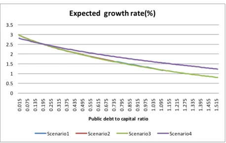
Growth decreases as private capital is crowded out by public debt, which decreases given (8’). Figure 6 gives the expected growth rate from the period t + 1 perspective. Tax increases (i.e., higher g) in the consolidation regime exert two opposing impacts on growth. As stated above, it serves to lower , which increases as accumulated at period t. The tax burden, on the other hand, reduces the output in the event of consolidation at period t+1 that is reflected in the bracket of the expectation in (9’). In comparison between Scenarios 1 and 2, the two yield almost the same growth rate for lower , and the latter experiences slightly higher growth after

= 0.4 than the former until the critical ratio in which the interior solution disappears in Scenario 2. The same can be seen when Scenario 3 is compared with Scenario 1. However, the difference is negligible. t t k k+1/ + t b * 1 + t R kt+1/kt 1 1/ + + t t k b 1/kt+1

Demography makes a considerable difference. The expected growth rate seen in Scenario 4 is initially lower than the benchmark scenario, but as the debt-to-capital ratio increases, the relationship is reversed and the difference expands as public debt is built up relative to capital. This may be counter-intuitive, but it is because the lower risk of fiscal consolidation serves to decrease the expected tax rate from the period t perspective. In addition, with GB interest rate being lowered, private capital accumulation is less crowded in Scenario 4, enhancing kt+1/kt.

Figure 7: Economic Growth

0 0.5 1 1.5 2 2.5 3 3.5 0. 0 15 0. 0 75 0. 1 35 0. 1 95 0. 2 55 0. 3 15 0. 3 75 0. 4 35 0. 4 95 0. 5 55 0. 6 15 0. 6 75 0. 7 35 0. 7 95 0. 9 75 1. 0 35 1. 0 95 1. 1 55 1. 5 15 blic debt to ca o

Expected growth rate(%)

0. 8 55 0. 9 15 pital rati 1. 2 15 1. 2 75 1. 3 35 1. 3 95 1. 4 55 Pu

5.3 Debt accumulation

(25)

Consider the dynamics of the public debt-to-capital ratio, which has been treated as exogenous in the previous subsection. In doing so, we divide , which is realized at t + 1 period into four classes and for each quartered group, and the (conditional) expected level of is calculated given a that is determined at period t. Note that the expectation is taken from the period t perspective. Table 2 shows the results in the benchmark scenario.

1 + t ε 2 2/ + + t t k b 1 1/ + + t t k b 1 1/ + + t t k b 1 + t

Table 2: Transition of Debt-to-capital Ratio

0.5~0.75 0.75~ 1.00~1.25 1.25~1.50 0.03 0.85 0. 0.10 0.02 0.06 1.10 0. 0.14 0.04 0.12 0. 0.22 0.10 0.18 0. 0.32 0.16 0.21 0. 0.37 0.19 0.24 1. 0.43 0.22 0.3 0.56 0.29 0.405 0.85 0.44 0.42 0.90 0.46 0.45 1.01 0.51 0.465 1.07 0.51 0.6 0.69 0.705 1.08 1.00 29 36 54 77 91 08 0.54 0.62 0.80 1.03 1 1/ + + t t k b 1 + t ε

The expected ratio of bt+2/kt+2_{is increasing with} _{and is higher for the lower quarter of}

ε . At the lowest quarter, that is, , the average of goes beyond the critical

ratio, =1.1, at which interior equilibrium ceases to exist according to Figure 2, when the debt-to-capital ratio is more than 0.06, implying that fiscal consolidation is inevitable at t+2 or ] 75 . 0 , 5 . 0 [ 1∈ + t ε bt+2/kt+2 + t b 2/kt+2 1 1/ + + t t k b ε = +2 t εˆ ε_t₊₁ 1 1/ + + t t k b t+1∈[1.25,1.5]

. In higher-quartered groups of , the expected ratio remains at sustainable level

for larger . For instance, at the highest quarter, that is, ε , interior

equilibrium survives at period t+1 for bt+1/kt+1 less than 0.72.

6.

Political Economy

We have so far assumed the process of accumulation of public debt as exogenous. One possible objection is that there should exist a self-correcting mechanism to contain public debt at sustainable levels by raising taxes and/or cutting expenditures. Indeed, rational voters may not allow the risk of fiscal crisis to deepen over time, but may undertake preventive measures to curtail such risk. In our OLG setting, however, the representative household of each generation with limited life span may