A Non-Parametric Approach to
Dynamic Programming
Oliver B. Kroemer1,2 Jan Peters1,2
1Intelligent Autonomous Systems, Technische Universität Darmstadt 2Robot Learning Lab, Max Planck Institute for Intelligent Systems
{kroemer,peters}@ias.tu-darmstadt.de
Abstract
In this paper, we consider the problem of policy evaluation for continuous-state systems. We present a non-parametric approach to policy evaluation, which uses kernel density estimation to represent the system. The true form of the value function for this model can be determined, and can be computed using Galerkin’s method. Furthermore, we also present a unified view of several well-known policy evaluation methods. In particular, we show that the same Galerkin method can be used to derive Least-Squares Temporal Difference learning, Kernelized Temporal Difference learning, and a discrete-state Dynamic Programming solution, as well as our proposed method. In a numerical evaluation of these algorithms, the proposed ap-proach performed better than the other methods.
1
Introduction
Value functions are an essential concept for determining optimal policies in both optimal con-trol [1] and reinforcement learning [2, 3]. Given the value function of a policy, an improved policy is straightforward to compute. The improved policy can subsequently be evaluated to obtain a new value function. This loop of computing value functions and determining better policies is known aspolicy iteration. However, the main bottleneck in policy iteration is the computation of the value function for a given policy. Using the Bellman equation, only two classes of systems have been solved exactly: tabular discrete state and action problems [4] as well as linear-quadratic regulation problems [5]. The exact computation of the value function remains an open problem for most systems with continuous state spaces [6]. This paper focuses on steps toward solving this problem.
As an alternative to exact solutions, approximate policy evaluation methods have been developed in reinforcement learning. These approaches includeMonte Carlo methods, tem-poral difference learning, andresidual gradient methods. However, Monte Carlo methods are well-known to have an excessively high variance [7, 2], and tend to overfit the value function to the sampled data [2]. When using function approximations, temporal difference learning can result in a biased solution[8]. Residual gradient approaches are biased unless multiple samples are taken from the same states [9], which is often not possible for real continuous systems.
In this paper, we propose a non-parametric method for continuous-state policy evaluation. The proposed method uses a kernel density estimate to represent the system in a flexible manner. Model-based approaches are known to be more data efficient than direct methods, and lead to better policies [10, 11]. We subsequently show that the true value function for this model has a Nadaraya-Watson kernel regression form [12, 13]. Using Galerkin’s projection method, we compute a closed-form solution for this regression problem. The
resulting method is calledNon-Parametric Dynamic Programming (NPDP), and is a stable as well as consistent approach to policy evaluation.
The second contribution of this paper is to provide a unified view of several sample-based algorithms for policy evaluation, including the NPDP algorithm. In Section 3, we show how Least-Squares Temporal Difference learning (LSTD) in [14],Kernelized Temporal Difference learning (KTD) in [15], and Discrete-State Dynamic Programming (DSDP) in [4, 16] can all be derived using the same Galerkin projection method used to derive NPDP. In Section 4, we compare these methods using empirical evaluations.
In reinforcement learning, the uncontrolled system is usually represented by a Markov De-cision Process (MDP). An MDP is defined by the following components: a set of states
S; a set of actions A; a transition distribution p(s0|a,s), where s0 ∈ S is the next state
given action a∈Ain state s∈S; a reward functionr, such thatr(s,a)is the immediate
reward obtained for performing actionain states; and a discount factorγ∈[0,1)on future
rewards. Actions a are selected according to the stochastic policy π(a|s). The goal is to
maximize the discounted rewards that are obtained; i.e., maxP∞
t=0γ
tr(s
t,at). The term
system will refer jointly to the agent’s policy and the MDP.
The value of a stateV(s), for a specific policyπ, is defined as the expected discounted sum
of rewards that an agent will receive after visiting statesand executing policyπ; i.e.,
V(s) =E P∞ t=0γ tr(s t,at) s0=s, π . (1)
By using the Markov property, Eq. (1) can be rewritten as theBellman equation
V(s) =´
A ´
Sπ(a|s)p(s
0|s,a) [r(s,a) +γVπ(s0)]ds0da. (2)
The advantage of using the Bellman equation is that it describes the relationship between the value function at one statesand its immediate follow-up statess0∼p(s0|s,a). In contrast,
the direct computation of Eq. (1) relies on the rewards obtained from entire trajectories.
2
Non-Parametric Model-based Dynamic Programming
We begin describing the NPDP approach by introducing the kernel density estimation frame-work used to represent the system. The true value function for this model has a kernel regression form, which can be computed by using Galerkin’s projection method. We subse-quently discuss some of the properties of this algorithm, including its consistency.
2.1 Non-Parametric System Modeling
The dynamics of a system are compactly represented by the joint distribution p(s,a,s0).
Using Bayes rule and marginalization, one can compute the transition probabilities
p(s0|s,a) and the current policy π(a|s) from this joint distribution; e.g. p(s0|s,a) =
p(s,a,s0)/´p(s,a,s0)ds0. Rather than assuming that certain prior information is given,
we will focus on the problem where only sampled information of the system is available. Hence, the system’s joint distribution is modeled from a set ofnsamples obtained from the
real system. The ith sample includes the current states
i ∈S, the selected actionai ∈A,
and the follow-up states0i ∈S, as well as the immediate rewardri ∈R. The state space S
and the action spaceAare assumed to be continuous.
We propose using kernel density estimation to represent the joint distribution [17, 18] in a non-parametric manner. Unlike parametric models, non-parametric approaches use the collected data as features, which leads to accurate representations of arbitrary functions [19]. The system’s joint distribution is therefore modeled as p(s,a,s0) =
n−1Pn
i=1ψi(s0)ϕi(a)φi(s), where ψi(s0) = ψ(s0,s0i), ϕi(a) = ϕ(a,ai), and φi(s) =
φ(s,si)are symmetric kernel functions. In practice, the kernel functionsψandφwill often
be the same. To ensure a valid probability density, each kernel must integrate to one; i.e., ´
φi(s)ds= 1,∀i, and similarly for ψandϕ. As an additional constraint, the kernel must
always be positive; i.e., ψi(s0)ϕi(a)φi(s)≥0, ∀s∈S. This representation implies a
fac-torization into separateψi(s0),ϕi(a), andφi(s)kernels. As a result, an individual sample
cannot express correlations between s0, a, and s. However, the representation does allow
The reward function r(s,a) must also be represented. Given the kernel density estimate
representation, the expected reward for a state-action pair is denoted as [12]
r(s,a) =E[r|s,a] = Pn k=1rkϕk(a)φk(s) Pn i=1ϕi(a)φi(s) .
Having specified the model of the system dynamics and rewards, the next step is to derive the corresponding value function.
2.2 Resulting Solution
In this section, we propose an approach to computing the value function for the continuous model specified in Section 2.1. Every policy has a unique value function, which fulfills the Bellman equation, Eq. (2), for all states [2, 20]. Hence, the goal is to solve the Bellman equation for the entire state space, and not just at the sampled states. This goal can be achieved by using the Galerkin projection method to compute the value function for the model [21].
The Galerkin method involves first projecting the integral equation into the space spanned by a set of basis functions. The integral equation is then solved in this projected space. To begin, the Bellman equation, Eq. (2), is rearranged as
V(s) = ´ A ´ Sπ(a|s)r(s,a)p(s 0|s,a)ds0da+´ S ´ Ap(s 0|s,a)γV (s0)π(a|s)dads0, p(s)V (s) = ˆ A p(a,s)r(s,a)da+γ ˆ S p(s0,s)V (s0)ds0. (3)
Before applying the Galerkin method, we derive the exact form of the value function. Ex-panding the reward function and joint distributions, as defined in Section 2.1, gives
p(s)V (s) = n−1 ˆ A Pn k=1ϕk(a)φk(s) Pn i=1riϕi(a)φi(s) Pn j=1ϕj(a)φj(s) da+γ ˆ S p(s0,s)V(s0)ds0, p(s)V (s) = ˆ A n−1Pn i=1riϕi(a)φi(s)da+γ ˆ S n−1Pn i=1ψi(s 0)φ i(s)V (s0)ds0, p(s)V (s) = n−1Pn i=1riφi(s) +n −1Pn i=1γ ˆ S ψi(s0)φi(s)V(s0)ds0, Therefore, p(s)V(s) = n−1Pn
i=1θiφi(s), where θ are value weights. Given that p(s) =
n−1Pn
j=1φj(s), the true value function of the kernel density estimate system has a
Nadaraya-Watson kernel regression [12, 13] form
V(s) = Pn i=1θiφi(s) Pn j=1φj(s) . (4)
Having computed the true form of the value function, the Galerkin projection method can be used to compute the value weightsθ. The projection is performed by taking the expectation
of the integral equation with respect to each of the n basis function φi. The resulting n
simultaneous equations can be written as the vector equation ˆ S φ(s)p(s)V(s)ds= ˆ S φ(s)n−1φ(s)Trds+γ ˆ S ˆ S φ(s)n−1φ(s)Tψ(s0)V(s0)ds0ds,
where the ith elements of the vectors are given by[r]i=r
i,[φ(s)]i=φi(s), and[ψ(s0)]i=
ψi(s0). Expanding the value functions gives
ˆ S φ(s)φ(s)Tθds= ˆ S φ(s)φ(s)Trds+γ ˆ S ˆ S φ(s)φ(s)Tψ(s0) φ(s 0)T θ Pn i=1φi(s0) ds0ds, Cθ=Cr+γCλθ, where C = ´ Sφ(s)φ(s) Td s, and λ =´ S( Pn i=1φi(s 0))−1ψ(s0)φ(s0)Td s0 is a stochastic
Algorithm 1Non-Parametric Dynamic Programming
Input: Computation:
nsystem samples: Reward vector:
statesi, next state s0i, and rewardri [r]i=ri
Kernel functions: Transition matrix:
φi(sj) =φ(si,sj), andψi s0j =ψ s0i,s0j [λ]i,j=´ S φj(s0)ψi(s0) Pn k=1φk(s0) ds0
Discount factor: Value weights:
0≤γ <1 θ= (I−γλ)−1r Output: Value function: V (s) = Pn i=1θiφi(s) Pn j=1φj(s)
are coincident. In such cases, there exists an infinite set of solutions forθ. However, all of
the solutions result in identical values. The NPDP algorithm uses the solution given by
θ= (I−γλ)−1r, (5)
which always exists for any stochastic matrix λ. Thus, the derivation has shown that the
exact value function for the model in Section 2.1 has a Nadaraya-Watson kernel regression form, as shown in Eq. (4), with weightsθ given by Eq. (5). The non-parametric dynamic
programming algorithm is summarized in Alg. 1. The NPDP algorithm ultimately requires only the state informationsands0, and not the actionsa. In Section 3, we will show how
this form of derivation can also be used to derive the LSTD, KTD, and DSDP algorithms. 2.3 Properties of the NPDP Algorithm
In this section, we discuss some of the key properties of the proposed NPDP algorithm, including precision, accuracy, and computational complexity. Precision refers to how close the predicted value function is to the true value function of the model, while accuracy refers to how close the model is to the true system.
One of the key contributions of this paper is providing the true form of the value function for policy evaluation with the non-parametric model described in Section 2.1. The parameters of this value function can be computed precisely by solving Eq. (5). Even ifλis evaluated
numerically, a high level of precision can still be obtained.
As a non-parametric method, the accuracy of the NPDP algorithm depends on the number of samples obtained from the system. It is important that the model, and thus the value function, converges to that of the true system as the number of samples increases; i.e., that the model is statistically consistent. In fact, kernel density estimation can be proven to have almost sure convergence to the true distribution for a wide range of kernels [22].
Given that λ is a stochastic matrix and 0 ≤γ <1, it is well-known that the inversion of (I−γλ) is well-defined [16]. The inversion can therefore also be expanded according to
the Neumann series; i.e., θ =P∞
i=0[γλ]
ir. Similar to other kernel-based policy evaluation
methods [23, 24], NPDP has a computational complexity ofO(n3)when performed naively.
However, by taking advantage of sparse matrix computations, this complexity can be reduced toO(nz), wherez is the number of non-zero elements in(I−γλ).
3
Relation to Existing Methods
The second contribution of this paper is to provide a unified view of Least Squares Temporal Difference learning (LSTD), Kernelized Temporal Difference learning (KTD), Discrete-State Dynamic Programming (DSDP), and the proposed Non-Parametric Dynamic Programming (NPDP). In this section, we utilize the Galerkin methodology from Section 2.2 to re-derive the LSTD, KTD, and DSDP algorithms, and discuss how these methods compare to NPDP. A numerical comparison is given in Section 4.
3.1 Least Squares Temporal Difference Learning
The LSTD algorithm allows the value functionV(s)to be represented by a set ofmarbitrary
basis functionsφˆ i(s), see [14]. Hence,V(s) =P m i=1θˆiφˆi(s) = ˆφ(s) T ˆ θ, whereθˆis a vector
of coefficients learned during policy evaluation, and [ ˆφ(s)]i= ˆφi(s). In order to re-derive
the LSTD policy evaluation, the joint distribution is represented as a set of delta functions
p(s,a,s0) =n−1Pn
i=1δi(s,a,s0), where δi(s,a,s0) is a Dirac delta function centered on
(si,ai,s0i). Using Galerkin’s method, the integral equation is projected into the space of
the basis functionsφˆ(s). Thus, Eq. (3) becomes
ˆ S ˆ φ(s)p(s) ˆφ(s)Tθˆds= ˆ A ˆ S ˆ φ(s)p(s,a)r(s,a)dsda+γ ˆ S ˆ φ(s)p(s,s0) ˆφ(s0)Tθˆds0ds, n X i=1 ˆ φ(si) ˆφ(si)Tθˆ= n X j=1 r(sj,aj) ˆφ(sj) +γ n X k=1 ˆ φ(sk) ˆφ(s0k) T ˆ θ, n X i=1 ˆ φ(si)φˆ(si)T −γφˆ(s0i) T ˆ θ= n X j=1 r(sj,aj) ˆφ(sj),
and thus Aθˆ = b, where A = Pn
i=1φˆ(si) ( ˆφ(si)
T
− γφˆ(s0i)T) and b =
Pn
j=1r(sj,aj) ˆφ(sj). The final weights are therefore given by
ˆ
θ=A−1b.
This equation is also solved by LSTD, including the incremental updates of A and b as
new samples are acquired [14]. Therefore, LSTD can be seen as computing the transitions between the basis functions using a Monte Carlo approach. However, Monte Carlo methods rely on large numbers of samples to obtain accurate results.
A key disadvantage of the LSTD method is the need to select a specific set of basis functions. The computed value function will always be a projection of the true value function into the space of these basis functions [8]. If the true value function does not lie within the space of these basis functions, the resulting approximation may be arbitrarily inaccurate, regardless of the number of acquired samples. However, using predefined basis functions only requires inverting anm×mmatrix, which results in a lower computational complexity than NPDP.
The LSTD may also need to be regularized, as the inversion ofAbecomes ill-posed if the
basis functions are too densely spaced. Regularization has a similar effect to changing the transition probabilities of the system [25].
3.2 Kernelized Temporal Difference Learning Methods
The proposed approach is of course not the first to use kernels for policy evaluation. Meth-ods such as kernelized least-squares temporal difference learning [24] and Gaussian process temporal difference learning [23] have also employed kernels in policy evaluation. Taylor and Parr demonstrated that these methods differ mainly in their use of regularization [15]. The unified view of these methods is referred to as Kernelized Temporal Difference learning. The KTD approach assumes that the reward and value functions can be represented by kernelized linear least-squares regression; i.e., r(s) = k(s)TK−1r and V(s) = k(s)Tθˆ,
where [k(s)]i =k(s,si), [K]ij =k(si,sj),[r]i =ri, and θˆis a weight vector. In order to
derive KTD using Galerkin’s method, it is necessary to again represent the joint distribution as p(s,a,s0) =n−1Pn
i=1δi(s,a,s0). The Galerkin method projects the integral equation
into the space of the Kronecker delta functions[δ(s)]iˇ = ˇδi(s,ai,si0), whereδˇi(s,a,s0) = 1
ifs0=s0i,a=ai, ands=si; otherwiseδˇi(s,a,s0) = 0. Thus, Eq. (3) becomes
ˆ S ˇ δ(s)p(s)k(s)Tθˆds= ˆ S ˇ δ(s)p(s)r(s)ds+γ ˆ S ˇ δ(s)p(s,s0)k(s0)Tθˆds0ds,
By substitutingp(s,a,s0)and applying the sifting property of delta functions, this equation becomes n X i=1 ˇ δ(si)k(si)Tθˆ= n X j=1 ˇ δ(sj)k(sj)TK−1r+γ n X k=1 ˇ δ(sk)k(s0k)Tθˆ,
and thusKθˆ=r+γK0θˆ, where[K0]ij=k(s0i,sj). The value function weights are therefore ˆ
θ= (K−γK0)−1r,
which is identical to the solution found by the KTD approach [15]. In this manner, the KTD approach computes a weighting θˆsuch that the difference in the value atsi and the
discounted value at s0i equals the observed empirical reward ri. Thus, only the finite set
of sampled states are regarded for policy evaluation. Therefore, some KTD methods, e.g. Gaussian process temporal difference learning [23], require that the samples are obtained from a single trajectory to ensure thats0i=si+1.
A key difference between KTD and NPDP is the representation of the value functionV(s).
The form of the value function is a direct result of the representation used to embody the state transitions. In the original paper [15], the KTD algorithm represents the transitions by using linear kernelized regression ˆk(s0) = k(s)TK−1K0, where [k(sˆ 0)]i =
E[k(s0,si)].
The value functionV(s) =k(s)Tθˆis the correct form for this transition model. However,
the transition model does not explicitly represent a conditional distribution and can lead to inaccurate predictions. For example, consider two samples that start at s1 = 0 and
s2 = 0.75 respectively, and both transition to s0 = 0.75. For clarity, we use a box-cart
kernel with a width of one k(si, sj) = 1iffksi−sjk ≤0.5and0 otherwise. Hence,K=I
and each row of K’ corresponds to (0,1). In the region 0.25 ≤ s ≤ 0.5, where the two
kernels overlap, the transition model would then predict ˆk(s) =k(s)TK−1K0 = [ 0
2 ].
This prediction is however impossible as it requires that E[k(s0, s2)] > maxsk(s, s2). In
comparison, NPDP would predict the distributionψ(s0)≡ψ1(s0)≡ψ2(s0)for all states in
the range−0.5≤s≤1.25.
Similar as for LSTD, the matrix(K−γK0)may become singular and thus not be invertible.
As a result, KTD usually needs to be regularized [15]. Given that KTD requires inverting ann×nmatrix, this approach has a computational complexity similar to NPDP.
3.3 Discrete-State Dynamic Programming
The standard tabular DSDP approach can also be derived using the Galerkin method. Given a system with q discrete states, the value function has the form V(s) = δ(s)ˇ Tv,
where δ(s)ˇ is a vector of qKronecker delta functions centered on the discrete states. The
corresponding reward function isr(s) =δ(s)ˇ T¯r. The joint distribution is given byp(s0,s) =
q−1δ(s)TP δ(s0), where P is a stochastic matrix Pq
j=1[P]ij = 1, ∀i and hence p(s) =
q−1Pq
i=1δi(s). Galerkin’s method projects the integral equation into the space of the
statesδ(s)ˇ . Thus, Eq. (3) becomes
ˆ S ˇ δ(s)p(s)δ(s)ˇ Tvds= ˆ S ˇ δ(s)p(s)δ(s)ˇ Tr¯ds+γ ˆ S ˇ δ(s)p(s,s0)δ(sˇ 0)Tvds0ds, Iv=Ir¯+γ ˆ S ˇ δ(s)δ(s)TP δ(s0)δ(sˇ 0)Tvds0ds, v=r¯+γP v, v= (I−γP)−1r¯, (6)
which is the same computation used by DSDP [16]. The DSDP and NPDP methods actually use similar models to represent the system. While NPDP uses a kernel density estimation, the DSDP algorithm uses a histogram representation. Hence, DSDP can be regarded as a special case of NPDP for discrete state systems.
The DSDP algorithm has also been the basis for continuous-state policy evaluation algo-rithms [26, 27]. These algoalgo-rithms first use the sampled states as the discrete states of an MDP and compute the corresponding values. The computed values are then generalized, under a smoothness assumption, to the rest of the state-space using local averaging. Unlike these methods, NPDP explicitly performs policy evaluation for a continuous set of states.
4
Numerical Evaluation
In this section, we compare the different policy evaluation methods discussed in the previous section, with the proposed NPDP method, on an illustrative benchmark system.
4.1 Benchmark Problem and Setup
In order to compare the LSTD, KTD, DSDP, and NPDP approaches, we evaluated the methods on a discrete-time continuous-state system. A standard linear-Gaussian system was used for the benchmark problem, with transitions given by s0 = 0.95s+ω where ω is
Gaussian noiseN(µ= 0, σ= 0.025). The initial states are restricted to the range0.95to1.
The reward functions consist of three Gaussians, as shown by the black line in Fig. 1. The KTD method was implemented using a Gaussian kernel function and regularization. The LSTD algorithm was implemented using 15 uniformly-spaced normalized Gaussian basis functions, and did not require regularization. The DSDP method was implemented by discretizing the state-space into 10 equally wide regions. The NPDP method was also implemented using Gaussian kernels.
The hyper-parameters of all four methods, including the number of basis functions for LSTD and DSDP, were carefully tuned to achieve the best performance. As a performance base-line, the values of the system in the range 0 < s < 1 were computed using a Monte
Carlo estimate based on50000trajectories. The policy evaluations performed by the tested
methods were always based on only500samples; i.e. 100times less samples than the
base-line. The experiment was run500times using independent sets of500samples. The samples
were not drawn from the same trajectory. 4.2 Results
The performance of the different methods were compared using three performance measures. Two of the performance measures are based on the weighted Mean Squared Error (MSE) [2] E(V) =´01W(s) (V(s)−V?(s))2dswhere V? is the true value function andW(s)≥0,
for all states, is a weighting distribution ´1
0 W(s)ds = 1. The first performance measure
Eunif corresponds to the MSE where W(s) = 1for all states in the range zero to one. The second performance measure Esamp corresponds to the MSE where W(s) = n−1Σni=1δi(s)
respectively. Thus,Esamp is an indicator of the accuracy in the space of the samples, while
Eunif is an indicator of how well the computed value function generalizes to the entire state space. The third performance measure Emax is given by the maximum error in the value function. This performance measure is the basis of a bound on the overall value function approximation [20].
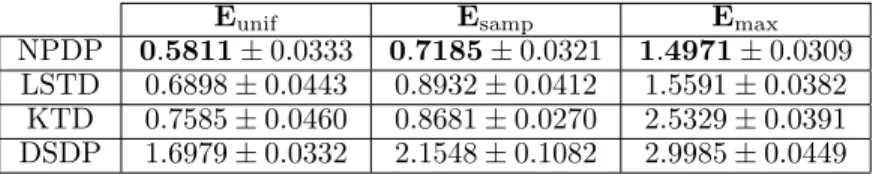
The results of the experiment are shown in Table 1. The performance measures were aver-aged over the500independent trials of the experiment. For all three performance measures,
the NPDP algorithm achieved the highest levels of performance, while the DSDP approach consistently led to the worst performance.
Eunif Esamp Emax
NPDP 0.5811±0.0333 0.7185±0.0321 1.4971±0.0309
LSTD 0.6898±0.0443 0.8932±0.0412 1.5591±0.0382
KTD 0.7585±0.0460 0.8681±0.0270 2.5329±0.0391
DSDP 1.6979±0.0332 2.1548±0.1082 2.9985±0.0449
Table 1: Each row corresponds to one of the four tested algorithms for policy evaluation. The columns indicate the performance of the approaches during the experiment. The per-formance indexes include the mean squared error evaluated uniformly over the zero to one range, the mean squared error evaluated at the 500 sampled points, and the maximum error. The results are averaged over 500 trials. The standard errors of the means are also given.
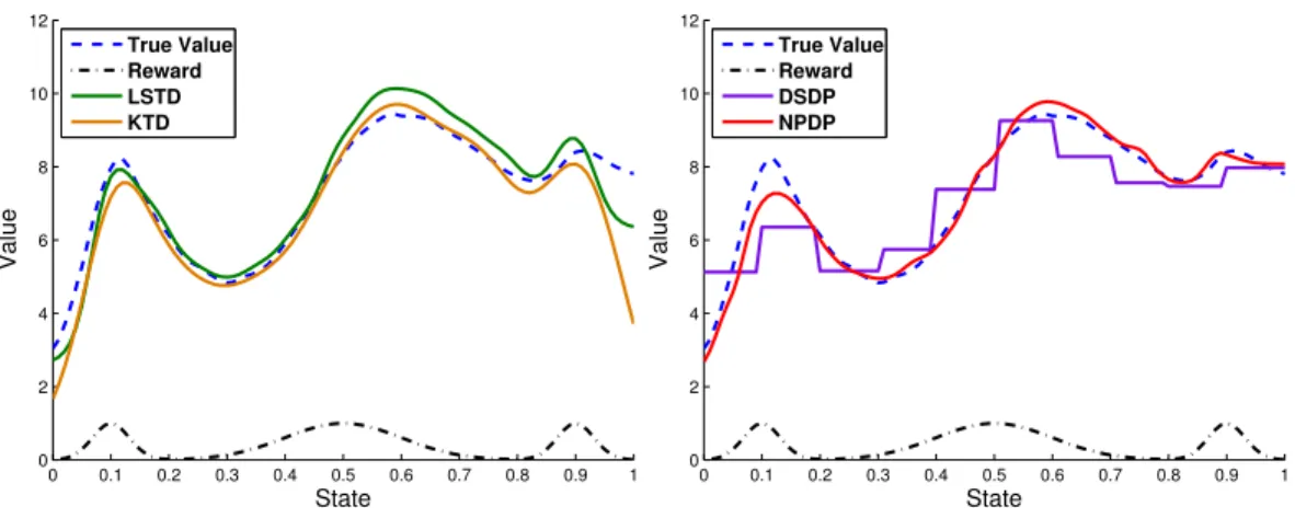
0 0.1 0.2 0.3 0.4 0.5 0.6 0.7 0.8 0.9 1 0 2 4 6 8 10 12 State Value True Value Reward LSTD KTD 0 0.1 0.2 0.3 0.4 0.5 0.6 0.7 0.8 0.9 1 0 2 4 6 8 10 12 State Value True Value Reward DSDP NPDP
Figure 1: Value functions obtained by the evaluated methods. The black lines show the reward function. The blue lines show the value function computed from the trajectories of
50,000uniformly sampled points. The LSTD, KTD, DSDP, and NPDP methods evaluated
the policy using only 500 points. The presentation was divided into two plots for improved clarity
4.3 Discussion
The LSTD algorithm achieved a relatively lowEunif value, which indicates that the tuned basis functions could accurately represent the true value function. However, the performance of LSTD is sensitive to the choice of basis functions and the number of samples per basis function. Using20basis functions instead of15reduces the performance of LSTD toEunif=
2.8705andEsamp= 1.0256as a result of overfitting. The KTD method achieved the second best performance forEsamp, as a result of using a non-parametric representation. However, the value tended to drop in sparsely-sampled regions, which lead to relatively high Eunif and Emax values. The discretization of states for DSDP is generally a disadvantage when modeling continuous systems, and resulted in poor overall performance for this evaluation. The NPDP approach out-performed the other methods in all three performance measures. The performance of NPDP could be further improved by using adaptive kernel density estimation [28] to locally adapt the kernels’ bandwidths according to the sampling density. However, all methods were restricted to using a single global bandwidth for the purpose of this comparison.
5
Conclusion
This paper presents two key contributions to continuous-state policy evaluation. The first contribution is the Non-Parametric Dynamic Programming algorithm for policy evaluation. The proposed method uses a kernel density estimate to generate a consistent representation of the system. It was shown that the true form of the value function for this model is given by a Nadaraya-Watson kernel regression. The NPDP algorithm provides a solution for calculating the value function. As a kernel-based approach, NPDP simultaneously addresses the problems of function approximation and policy evaluation.
The second contribution of this paper is providing a unified view of Least-Squares Temporal Difference learning, Kernelized Temporal Difference learning, and discrete-state Dynamic Programming, as well as NPDP. All four approaches can be derived from the Bellman equation using the Galerkin projection method. These four approaches were also evaluated and compared on an empirical problem with a continuous state space and non-linear reward function, wherein the NPDP algorithm out-performed the other methods.
Acknowledgements
The project receives funding from the European Community’s Seventh Framework Pro-gramme under grant agreement n° ICT- 248273 GeRT and n° 270327 Complacs.
References
[1] Dimitri P. Bertsekas. Dynamic Programming and Optimal Control, Vol. II. Athena Scientific, 2007.
[2] R. S. Sutton and A. G. Barto. Reinforcement Learning: An Introduction. 1998.
[3] H. Maei, C. Szepesvari, S. Bhatnagar, D. Precup, D. Silver, and R. Sutton. Convergent temporal-difference learning with arbitrary smooth function approximation. InNIPS, pages 1204–1212, 2009.
[4] Richard Bellman. Bottleneck problems and dynamic programming.Proceedings of the National
Academy of Sciences of the United States of America, 39(9):947–951, 1953.
[5] R.E. Kalman. Contributions to the theory of optimal control, 1960.
[6] Warren B. Powell.Approximate Dynamic Programming: Solving the Curses of Dimensionality
(Wiley Series in Probability and Statistics). Wiley-Interscience, 2007.
[7] Rémi Munos. Geometric Variance Reduction in Markov Chains: Application to Value Function and Gradient Estimation. Journal of Machine Learning Research, 7:413–427, 2006.
[8] Ralf Schoknecht. Optimality of reinforcement learning algorithms with linear function approx-imation. InNIPS, pages 1555–1562, 2002.
[9] Leemon Baird. Residual algorithms: Reinforcement learning with function approximation. In
ICML, 1995.
[10] Christopher G. Atkeson and Juan C. Santamaria. A Comparison of Direct and Model-Based Reinforcement Learning. InICRA, pages 3557–3564, 1997.
[11] H. Bersini and V. Gorrini. Three connectionist implementations of dynamic programming for optimal control: A preliminary comparative analysis. InNicrosp, 1996.
[12] E. Nadaraya. On estimating regression. Theory of Prob. and Appl., 9:141–142, 1964. [13] G. Watson. Smooth regression analysis. Sankhya, Series, A(26):359–372, 1964.
[14] Justin A. Boyan. Least-squares temporal difference learning. In ICML, pages 49–56, San Francisco, CA, USA, 1999. Morgan Kaufmann Publishers Inc.
[15] Taylor, Gavin and Parr, Ronald. Kernelized value function approximation for reinforcement learning. InICML, pages 1017–1024, New York, NY, USA, 2009. ACM.
[16] Dimitri P. Bertsekas and John N. Tsitsiklis. Neuro-Dynamic Programming. Athena Scientific, 1996.
[17] Murray Rosenblatt. Remarks on Some Nonparametric Estimates of a Density Function. The
Annals of Mathematical Statistics, 27(3):832–837, September 1956.
[18] Emanuel Parzen. On Estimation of a Probability Density Function and Mode. The Annals of
Mathematical Statistics, 33(3):1065–1076, 1962.
[19] G. S. Kimeldorf and G. Wahba. Some results on Tchebycheffian spline functions. Journal of
Mathematical Analysis and Applications, 33(1):82–95, 1971.
[20] Rémi Munos. Error bounds for approximate policy iteration. InICML, pages 560–567, 2003. [21] Kendall E. Atkinson. The Numerical Solution of Integral Equations of the Second Kind.
Cam-bridge University Press, 1997.
[22] Dominik Wied and Rafael Weissbach. Consistency of the kernel density estimator: a survey.
Statistical Papers, pages 1–21, 2010.
[23] Yaakov Engel, Shie Mannor, and Ron Meir. Reinforcement learning with Gaussian processes. InICML, pages 201–208, New York, NY, USA, 2005. ACM.
[24] Xin Xu, Tau Xie, Dewen Hu, and Xicheng Lu. Kernel least-squares temporal difference
learn-ing. International Journal of Information Technology, 11:54–63, 1997.
[25] J. Zico Kolter and Andrew Y. Ng. Regularization and feature selection in least-squares tem-poral difference learning. InICML, pages 521–528. ACM, 2009.
[26] Nicholas K. Jong and Peter Stone. Model-based function approximation for reinforcement learning. InAAMAS, May 2007.
[27] Dirk Ormoneit and Śaunak Sen. Kernel-Based reinforcement learning. Machine Learning, 49(2):161–178, November 2002.