Empirical Bayes Estimators for Sparse Sequences
K. Pavan Srinath
University of Cambridge, UK [email protected]Ramji Venkataramanan
University of Cambridge, UK [email protected]Abstract—The problem of estimating a high-dimensional sparse vectorθ∈Rnfrom an observation in i.i.d. Gaussian noise
is considered. An empirical Bayes shrinkage estimator, derived using a Bernoulli-Gaussian prior, is analyzed and compared with the well-known soft-thresholding estimator using squared-error loss as a measure of performance. We obtain concentration inequalities for the Stein’s unbiased risk estimate and the loss function of both estimators.
Depending on the underlyingθ, either the proposed empirical Bayes (eBayes) estimator or soft-thresholding may have smaller loss. We consider a hybrid estimator that attempts to pick the better of the soft-thresholding estimator and the eBayes estimator by comparing their risk estimates. It is shown that: i) the loss of the hybrid estimator concentrates on the minimum of the losses of the two competing estimators, and ii) the risk of the hybrid estimator is within order1/√nof the minimum of the two risks. Simulation results are provided to support the theoretical results.
I. INTRODUCTION
Consider the problem of estimating a sparse vectorθ∈Rn from a noisy observationy of the form
y=θ+w. (1) The noise vector w ∈ Rn is distributed as N(0,I) (by
rescalingyby1/σ, the case wherew∼ N(0, σ2I)reduces to the above form withθ/σ to be estimated). In this paper, as a measure of the performance of an estimatorˆθ, we consider the squared-error loss function given byL(θ,ˆθ(y)) :=kθˆ(y)− θk2, where k·k denotes the Euclidean norm. Therisk of the estimator for a given θ is the expected value of the loss function:
R(θ,θˆ) :=E h
kθˆ(y)−θk2i.
We emphasize thatθis deterministic, so the expectation above is computed over y∼ N(θ,I).
We assume thatθ has knon-zero entries out of n, where
kmay not be known to the estimator. Though our results are general, they are most interesting for the case where k = Θ(n). Thus as n gets large, the sparsity level η := k/n is bounded above and below by arbitrary constants in(0,1].
The sparse estimation problem has been widely studied [1]–[7] due to its fundamental role in non-parametric function estimation. If the function has a sparse representation in an orthogonal basis (e.g., a Fourier or wavelet basis), then (1) models the problem of estimating the function from a noisy measurement of n basis coefficients. Another motivation for constructing good sparse estimators comes from Approximate Message Passing (AMP) algorithms for compressed sensing, which is discussed in Sec. V-A.
The soft thresholding estimator is a popular choice of estimator when θ is assumed to be sparse [1]–[3], [7], [8], and is given as follows for thresholdλ. Fori∈ {1,2,· · ·, n},
ˆ θST ,i(yi;λ) = yi−λ ifyi > λ 0, if −λ≤yi ≤λ yi+λ ifyi <−λ.
Along with its simplicity, the soft-thresholding estimator has other attractive properties. For example, when n is large and the sparsity level η=k/n→0, the worst-case risk over the set of η-sparse vectors is2ηlogη−1(1 +o(1)). However, no sharp theoretical bounds exist for the risk of the soft-thresholding estimators for moderate or large values of η.
A. Motivation and Contributions
The well-known (positive-part) James-Stein estimator [9] for estimating an arbitrary θ ∈Rn from an observationy= θ+w, w∼ N(0,I), is given by ˆ θJ S = 1−n−2 kyk2 + y, (2) whereX+denotesmax(0, X). The James-Stein estimator has uniformly lower risk than the maximum-likelihood estimator ˆ
θ(y) = y (see, e.g., [10, Chap. 5]). An empirical Bayes viewpoint of this estimator is provided in [11]: assuming a Gaussian prior on θ so that θ ∼ N(0, ξ2I), the Bayes estimator is ˆ θBayes= 1− 1 1 +ξ2 y. (3) Based on the Gaussian prior, we have y ∼ N(0,(1 +ξ2)I). So,(n−2)/kyk2 is an unbiased estimate of1/(1 +ξ2), i.e.,
E(n−2)/kyk2= 1/(1 +ξ2).Plugging in this estimate of
1/(1+ξ2)in (3) (and ensuring that it is always≤1) givesθˆJ S in (2). One can also start with a Gaussian prior with non-zero mean, i.e., θ ∼ N(µ1, ξ2I), and use P
iyi/n as a plug-in estimate forµ. The resulting empirical Bayes estimator is the positive-part Lindley’s estimator [11].
This empirical Bayes derivation of the James-Stein estima-tor serves as a motivation for our work. In our setting, since we know that θ is sparse, we consider an empirical Bayes estimator based on a prior that is a mixture of a point mass at 0 and a continuous distribution with densityψ(θ;µ, ξ), where
µ is a location parameter (mean) and ξ is a scale parameter. The prior is given by
The parameter∈[0,1], which controls the sparsity, is treated as a fixed parameter that can be optimized. In particular,
need notbe the true sparsity levelη(which may be unknown). Takingψ to be the Gaussian density, in Sec. II we derive an empirical Bayes (eBayes) estimator using plug-in estimates for
µandξ2. In Sec. III, we derive a risk function estimate for the eBayes estimator using Stein’s unbiased risk estimate (SURE). We then consider a hybrid estimator which chooses between the eBayes estimator and the soft-thresholding estimator by comparing their risk estimates.
Sec. IV contains the main theoretical results of the paper. Theorem 1 shows that for largen, the SURE concentrates on a deterministic value which is within O(1/√n) of the true risk. Theorem 2 shows that the loss of the eBayes estimator concentrates on a deterministic value that is also within
O(1/√n) of the risk. Using these results (and analogous ones for soft-thresholding), Theorem 5 shows that for the hybrid estimator, the loss concentrates on the minimum of the losses of the two rival estimators, and its risk is within
O(1/√n) of the minimum of the two risks. In Section V, we provide simulation results, including an application of the hybrid estimator in the approximate message passing (AMP) algorithm for compressed sensing.
B. Related Work
In the context of wavelets, several works have considered estimators based on a signal prior that is a mixture of a point mass at0and a Gaussian distribution (see, e.g., [12]). In most of these works, the hyperparameters of the prior are chosen based on some prior information about the signal. Empirical Bayes estimators based on a prior that is a mixture of a point mass at0 and a distribution with a heavy-tailed density have been proposed in [3], [4]. The weights of the mixture are first determined using marginal log-likelihood; the estimator then uses a thresholding rule based on the posterior median. It has been shown that the risk of this estimator over the class of
η-sparse vectors is within a constant factor of the minimax risk when the sparsity levelη is small enough.
In this paper, we use a fixed mixture weight for the em-pirical Bayes estimator and emem-pirically estimate the location and scale parameters of the continuous part of the prior. This approach allows us to obtain concentration inequalities for the risk estimates, which then lead to a risk bound for the hybrid estimator.
Notation: The set {1,2,· · · , n} is denoted by [n]. Bold lowercase (uppercase) letters are used to denote vectors (matri-ces), and plain lowercase letters for their entries. For example, the entries ofyareyi,i= 1,· · ·, n. The indicator function of an event E is denoted by 1{E}. For positive-valued functions
f(n) and g(n), the notation f(n) = O(g(n)) means that
∃k >0 such that∀n > n0,f(n)≤kg(n). II. EMPIRICALBAYESESTIMATOR
Assuming that {θi}, i∈[n], were generated i.i.d. ∼f in (4), the conditional mean ofθgivenyis the optimal estimator (for squared-error loss). The empirical Bayes estimator for a
fixed ∈ [0,1] is this conditional mean, with the values of
µ, ξ estimated from the datay. Hence,∀i∈[n], ˆ θEB,i(y;) = R Rxf(x;,µ,ˆ ˆ ξ)φ(yi−x)dx R Rf(x;,µ,ˆ ˆ ξ)φ(yi−x)dx . (5) In (5),φ(x) := √1 2πe −x2/2
is the standard normal density, and ˆ
µ,ξˆare the estimates of µ, ξ fromy. A consistent estimator for µ(converging in probability toµ) is
ˆ
µ(y) = ¯y/, (6) where the empirical meany¯:=P
iyi/n. The scale parameter can be estimated using the second momenty2:=kyk2/nand the first moment y¯. In this paper, we consider the Gaussian density forψ so that
ψ(θ;µ, ξ) =p1
2πξ2exp(−(θ−µ) 2/2ξ2).
The meanµis estimated as in (6), andξ2, being the variance, is estimated as b ξ2(y) = 1 y2−(¯y) 2 −1 + .
The resulting empirical Bayes estimator is, fori∈[n],
ˆ θEB,i(y;) = ˆ µ+1− 1 1+ξb2 (yi−µˆ) 1 +(1− ) q 1 +ξb2exp (y i−µˆ)2 2(1+ξb2) −y2i 2 . (7)
For = 1, θˆEB reduces to the well-known James-Stein estimator [9], [13] that shrinks each element of y towards the empirical meany¯.
Note that ˆθEB is a shrinkage estimator — it shrinks each yi towards a common element µˆ, with the amount of shrinkage depending onyi. There are two terms that determine the shrinkage, the first being the term h1− 1
1+ξb2
i
which is common for all the yi. The second term influencing the shrinkage is the exponential in the denominator which depends on yi ; the smalleryi is, the smaller θi is expected to be and hence, the larger the amount of shrinkage.
III. RISKESTIMATORS AND THEHYBRID ESTIMATOR
Depending on the underlyingθ, either ˆθST or θˆEB may have smaller loss. To construct a hybrid estimator that reliably chooses the better estimator, we use Stein’s unbiased risk estimate (SURE) [14] to estimate the losses of each estimator.
Fact 1: [14] If an estimator θˆ(y) is almost everywhere differentiable, then the SURE of θˆ, given by
ˆ R(θ,θˆ(y)) :=−n+ky−θˆk2+ 2 n X i=1 ∂θˆi ∂yi ,
is an unbiased estimate of the risk R(θ,θˆ), i.e.,
E[ ˆR(θ,θˆ(y))] =R(θ,ˆθ).
Both the risk estimate and the loss function of an estimator ˆ
not explicitly indicate the dependency of the two on y. The normalized SURE forθˆST with threshold λis given by
ˆ R(θ,ˆθST;λ) n =−1 + ky−θˆSTk2 n + 2 n n X i=1 1{y2 i>λ2}. (8)
To keep the exposition simple, for our concentration re-sults we assume that the location parameter µˆ in θˆEB is zero. Extending the results to the case with a general µˆ is straightforward, though a bit cumbersome. Using SURE, the normalized risk estimate forˆθEB withµˆ= 0 is
ˆ R(θ,θˆEB;) n = kyk2 n −1 +a 2 y n n X i=1 yi2 1 + 2cye− ayyi2 2 b2 i(y) −2ay n n X i=1 y2i −1 bi(y) + 4 d2 yn2 n X i=1 y2 i bi(y) 1{kyk2>n}+ 2(1−)ay d3y/22n2 n X i=1 y4 ie− ayy2i 2 b2 i(y) −2(1p−)ay dy2n2 n X i=1 y2 ie− ayy2i 2 b2i(y) (9) where ay: = b ξ2 1 +ξb2 = 1− (kyk2/n−1)++ , dy: = 1 +ξb2= 1 + 1 kyk2 n −1 + , cy: = 1− q 1 +ξb2= 1− p dy, bi(y) : = 1 +cye− ayy2i 2 .
For largen, it is shown in [15, Lemma 4.1] that the last three terms in (9) each concentrate around deterministic constants of order 1/n. These terms can therefore be neglected in a practical application of the risk estimate.
We use the risk estimates in (8) and (9) to define a hybrid estimator that aims to select the estimator with smaller loss for theθ in context. The hybrid estimator is defined as
ˆ θH=γyθˆEB+ (1−γy)ˆθST, (10) where γy= 1 if Rˆ(θ,ˆθEB)≤Rˆ(θ,ˆθST), 0 otherwise. (11)
In the next section, we present concentration results for the risk estimates and loss functions ofθˆST andθˆEB, and use these to show that the loss of the hybrid estimator concentrates on the minimum of the losses of the two estimators. Due to space constraints, we omit the proofs, which can be found in Sections 4 and 6 of [15].
IV. MAINRESULTS
The constants in our concentration results for the eBayes estimator depend onθ via n1Pn
i=1θ 4
i. In order to make these constants universal, we assume that the fourth moment of θ
is bounded.
Assumption A: There exists a finite constantΛ>0 such that 1 n Pn i=1θ 4 i ≤Λ.
When Assumption A is satisfied, the constants in the concentration results depend only on Λ (and not on the underlyingθorn). For brevity, we henceforth do not explicitly indicate the dependence onλandin the notation for the risk estimates on the LHS of (8) and (9), respectively.
Theorem 1: Consider a sequence of θ with increasing dimension n and satisfying Assumption A. Then the risk estimateRˆ(θ,θˆEB)satisfies the following for anyt >0:
P 1 n ˆ R(θ,θˆEB)−R1(θ,θˆEB) ≥t ≤Ke−nkmin(t,t2)
where 0 < K ≤ 24 and k > 0 are absolute constants, and
R1(θ,ˆθEB)is a deterministic quantity such that
R1(θ,ˆθEB) n − R(θ,ˆθEB) n =O 1 √ n .
The next result shows that, like the risk estimate, the nor-malized loss of the eBayes estimator also concentrates on a deterministic value close to the true risk.
Theorem 2: Consider a sequence of θ with increasing dimension n and satisfying Assumption A. Then the loss function L(θ,θˆEB) = kθ−θˆEBk2 satisfies the following for any t >0: P 1 n L(θ, ˆ θEB)−R2(θ,ˆθEB) ≥t ≤Ke−nkmin(t,t2)
where K ≤ 10 and k are absolute positive constants, and
R2(θ,ˆθEB)is a deterministic quantity such that
R2(θ,ˆθEB) n − R(θ,ˆθEB) n =O 1 √ n .
The normalized SURE and the normalized loss for θˆST with threshold λsatisfy the following:
Theorem 3: [8] The SURE Rˆ(θ,ˆθST;λ) for the soft-thresholding estimator with parameter λ satisfies, for any
t >0, P 1 n ˆ R(θ,θˆST)−R(θ,θˆST) ≥t ≤2e− 2t 2 9(1+λ2 )2.
Theorem 4: The loss function L(θ,ˆθST) = kθ−ˆθSTk2 of the soft-thresholding estimator satisfies the following for any t >0: P 1 n L(θ, ˆ θST)−R(θ,ˆθST) ≥t ≤2e−nkmin(t,t2)
For a givenθ, let Lmin(θ,y) := min n L(θ,ˆθEB), L(θ,θˆST) o , κn:= 1 n R1(θ, ˆ θEB)−R2(θ,ˆθEB) ,
where R1(θ,θˆEB) and R2(θ,θˆEB) are the deterministic concentrating values in Theorems 1 and 2, respectively. Note thatκnis anO(1/
√
n)quantity since bothR1(θ,θˆEB)/nand R2(θ,θˆEB)/nare within O(1/
√
n)fromR(θ,ˆθEB)/n. The following theorem characterizes the lossL(θ,ˆθH(y))and the risk R(θ,θˆH)of the hybrid estimator.
Theorem 5: Consider a sequence of θ with increasing dimension n and satisfying Assumption A. Then, for any
t >0, we have P L(θ,ˆθH) n ≥ Lmin(θ,y) n +t+κn ! ≤Ke−nkmin(t,t2),
for some absolute positive constantsKandk. The risk of the hybrid estimator can be bounded as
R(θ,ˆθH) n ≤ 1 nmin n R(θ,θˆEB), R(θ,ˆθST) o +O 1 √ n . V. SIMULATIONRESULTS
When the true sparsity level η is unknown, one can optimize SURE to find the best fit for both θˆST and θˆEB. The concentration results (Theorems 1 and 3) imply that the SURE for either estimator does not deviate much from the actual risk for large n. SureShrink, proposed in [8], chooses the thresholding parameterλ∗as follows, from a setS that is a discretized version of the interval(0,√2 logn].
λ∗= arg min
λ∈S
ˆ
R(θ,θˆST;λ)/n (12)
whereRˆ(θ,θˆST;λ)is defined in (8).
We propose to find the best value of in (7) by first discretizing the set (0,1] (denoting it by D), and choosing the sparsity parameter as
∗= arg min
∈D
ˆ
R(θ,ˆθEB;)/n. (13)
HereRˆ(θ,θˆEB;)/n is as in (9), with suitable modifications to account for non-zeroµˆ. The hybrid estimator then chooses the estimator with lower value of SURE (Rˆ(θ,θˆST;λ∗) vs.
ˆ
R(θ,ˆθEB;∗)).
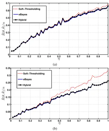
Fig. 1 shows the average normalized loss R˜(θ,θˆ)/n (av-eraged over 100 realizations of w) of the three estimators at different sparsity levels for two choices of the distribution of the non-zero entries of θ. We assume that the actual sparsity factor η is unknown and use SURE to find the best sparsity parameters for θˆST and ˆθEB. The optimization is performed over the discrete sets D = {0.02i, i ∈ [50]} and
S = {0.1i, i ∈ [d10√2 logne]}. In all the plots, n = 1000. Additional simulation plots, including fornas low as 50, are provided in [15, Section 5]. The plots suggest that for a wide range of θ,θˆEB is at least as good asθˆST for all values of the sparsity factorη, and better in most cases.
0 0.1 0.2 0.3 0.4 0.5 0.6 0.7 0.8 0.9 1 0 0.1 0.2 0.3 0.4 0.5 0.6 0.7 ˜R( θ , ˆθ)/n η Soft−Thresholding eBayes Hybrid (a) 0 0.1 0.2 0.3 0.4 0.5 0.6 0.7 0.8 0.9 1 0 0.05 0.1 0.15 0.2 0.25 0.3 0.35 η ˜R( θ , ˆθ)/n Soft−Thresholding eBayes Hybrid (b)
Fig. 1. Average normalized lossR˜(θ,θˆ)/nwithn= 1000for the following cases: a) The non-zero entries are drawn from the Laplace distribution with mean0and variance2. b) The non-zero entries are drawn from the uniform distribution on the interval[−2,2].
A. Application to Compressed Sensing
In compressed sensing, the goal is to estimate a sparse vector θ ∈Rn from a noisy linear measurementy ∈Rm of
the form
y=Aθ+w.
Assume that A is an m×n random matrix with i.i.d. sub-Gaussian entries with variance 1/m, and the noise vector
w ∼ N(0, σ2I). The undersampling ratio is denoted by
δ:=m/n <1.
For this model, Approximate Message Passing (AMP) [16]–[18] is a class of iterative algorithms to estimateθ from
y. Starting with the initial conditionsθ0 =0,z0=y, AMP iteratively produces estimates {θt+1}t≥0 as follows [17]:
θt+1=ft ATzt+θt (14) zt+1=y−Aθt+1+ 1 δzt ft0 ATzt+θt. Here for each t, ft : R → R is a “denoising” function, ft0 denotes its derivative, and both functions act component-wise on vectors. Foru∈Rn,huidenotes the average of its entries. The AMP update (14) is underpinned by the following key property of the effective observation vector (ATz
t+θt): for large n, after each iterationt, (ATz
t+θt)is approximately distributed as θ+τtZ, where Z∈Rn is a standard Gaussian
vector that is independent ofθ. The effective noise varianceτ2
t is determined (in the large system limit) by a scalar recursion
called state evolution [17]. For our purposes, it suffices to note that a good estimate ofτ2
t is given by bτ
2
t :=kzt
2
k/m. The function ft estimates the sparse vector θ from an observation in Gaussian noise of variance approximately bτt2. Therefore, in each iteration, the AMP provides a platform to compare the performance of soft-thresholding and the eBayes estimator (and hence the hybrid estimator) as choices forft. We note that while soft-thresholding operates on a vector component-wise, the eBayes estimator doesn’t. However, for sufficiently large values of m and n, both µˆ and ξb2 in
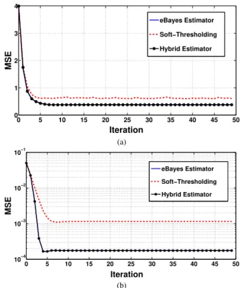
(6)-(7) are close to deterministic values in which case the eBayes estimator also approximately acts component-wise on a vector. The simulation plots in Fig. 2 show the performances of the three estimators when used in the AMP algorithm. We fix n= 10000 and consider two set-ups, which differ in the undersampling ratio δ = m/n, sparsity factor η = kθk0/n, noise varianceσ2, and the non-zero values ofθ. The measure-ment matrixA is chosen with its entries i.i.d.∼ N(0,1/m), and the sparsity factor η is assumed to be unknown. So, at each step of the algorithm, a suitable thresholdλ∗i (for soft-thresholding) and a suitable sparsity parameter ∗i (for the eBayes estimator) are chosen as described in (12) and (13) with the only difference being that the optimization is now based on kztk2/n, and not on SURE. A precise description of the algorithm can be found in [15, Section 5.1].
The plots in Fig. 2 show the progression of the mean squared error (MSE) kθt−θk2/n with the AMP iteration number t for the three estimators when applied in the AMP algorithm for compressed sensing. It can be inferred that the eBayes estimator provides a strong alternative to soft-thresholding in the AMP.
VI. CONCLUDINGREMARKS
For the problem of estimating a sparse vector (with possi-bly unknown sparsity level), we proposed an empirical Bayes estimator based on a Bernoulli-Gaussian prior. By obtaining a concentration inequality for its risk estimate (SURE), we showed that the risk of the hybrid estimator is close to the minimum of the risks of the competing estimators.
More generally, the approach of Theorem 5 could be used to bound the risk of a hybrid estimator that picks one among several estimators, provided one has concentration bounds for the risk estimates of each of the competing estimators. This suggests that an interesting direction for research is to obtain concentration bounds for the risk estimates of other useful estimators whose parameters depend on the data, e.g., an empirical Bayes estimator based on a Bernoulli-Laplace prior.
REFERENCES
[1] D. L. Donoho and I. M. Johnstone, “Ideal Spatial Adaptation by Wavelet Shrinkage,”Biometrika, vol. 81, no. 3, pp. 425–455, 1994.
[2] D. L. Donoho and I. M. Johnstone, “Minimax risk overlp-balls for
lq-error,”Probab. Th. Rel. Fields, vol. 99, pp. 277–303, 1994.
[3] I. M. Johnstone and B. W. Silverman, “Needles and straw in haystacks: Empirical Bayes estimates of possibly sparse sequences,” Ann. Stat., vol. 32, no. 4, pp. 1594–1649, 2004.
[4] I. M. Johnstone and B. W. Silverman, “Empirical Bayes selection of wavelet thresholds,”Ann. Stat., vol. 33, no. 4, pp. 1700–1752, 2005.
0 5 10 15 20 25 30 35 40 45 50 0 1 2 3 4 Iteration MSE eBayes Estimator Soft−Thresholding Hybrid Estimator (a) 0 5 10 15 20 25 30 35 40 45 50 10−4 10−3 10−2 10−1 Iteration MSE eBayes Estimator Soft−Thresholding Hybrid Estimator (b)
Fig. 2. Plots of the mean squared errorkθt−θk2/nas a function of the
iteration numbertfor the following cases: a)δ= 0.65,= 0.13,σ= 1, the non-zero entries ofθare drawn from N(0,5). b)δ= 0.5,= 0.05,
σ= 0.05, the non-zero entries are drawn from the Rademacher distribution.
[5] G. Leung and A. R. Barron, “Information Theory and Mixing Least-Squares Regressions,”IEEE Trans. Inf. Theory, vol. 52, pp. 3396–3410, August 2006.
[6] C. Carvalho, N. Polson, and J. G. Scott, “The horseshoe estimator for sparse signals,”Biometrika, vol. 97, no. 2, pp. 465–480, 2010. [7] I. M. Johnstone, Gaussian estimation: Sequence and wavelet
mod-els. Monograph, Available [Online]: http://statweb.stanford.edu/∼imj/ GE09-08-15.pdf, 2015.
[8] D. L. Donoho and I. M. Johnstone, “Adapting to Unknown Smoothness via Wavelet Shrinkage,”J. Amer. Stat. Assoc., vol. 90, pp. 1200–1224, Dec. 1995.
[9] W. James and C. M. Stein, “Estimation with Quadratic Loss,” inProc.
Fourth Berkeley Symp. Math. Stat. Probab., pp. 361–380, 1961.
[10] E. L. Lehmann and G. Casella, Theory of Point Estimation. Springer, New York, NY, 1998.
[11] B. Efron and C. Morris, “Data Analysis Using Stein’s Estimator and Its Generalizations,”J. Amer. Statist. Assoc., vol. 70, pp. 311–319, 1975. [12] F. Abramovich, T. Sapatinas, and B. W. Silverman, “Wavelet
threshold-ing via a Bayesian approach,”Journal of the Royal Statistical Society:
Series B (Statistical Methodology), vol. 60, no. 4, pp. 725–749, 1998.
[13] D. V. Lindley, “Discussion on Professor Stein’s Paper,”J. R. Stat. Soc., vol. 24, pp. 285–287, 1962.
[14] C. Stein, “Estimation of the mean of a multivariate normal distribution,”
Ann. Stat., vol. 9, pp. 1135–1151, 1981.
[15] K. P. Srinath and R. Venkataramanan, “Empirical bayes estimators for high-dimensional sparse vectors,”https:// arxiv.org/ abs/ 1707.09161, 2017.
[16] D. L. Donoho, A. Maleki, and A. Montanari, “Message-passing algo-rithms for compressed sensing,”Proceedings of the National Academy
of Sciences, vol. 106, no. 45, pp. 18914–18919, 2009.
[17] M. Bayati and A. Montanari, “The dynamics of message passing on dense graphs, with applications to compressed sensing,” IEEE Trans.
Inf. Theory, vol. 57, no. 2, pp. 764–785, 2011.
[18] S. Rangan, “Generalized approximate message passing for estimation with random linear mixing,” in Proc. IEEE Int. Symp. Inf. Theory, pp. 2168–2172, 2011.