04 August 2020
Selecting the Best Reliability Model to Predict Residual Defects in Open Source Software / ULLAH, NAJEEB; MORISIO, MAURIZIO; VETRO', ANTONIO. - In: COMPUTER. - ISSN 0018-9162. - 48:6(2015), pp. 50-58.
Original
Selecting the Best Reliability Model to Predict Residual Defects in Open Source Software
ieee Publisher: Published DOI:10.1109/MC.2013.446 Terms of use: openAccess Publisher copyright
copyright 20xx IEEE. Personal use of this material is permitted. Permission from IEEE must be obtained for all other uses, in any current or future media, including reprinting/republishing this material for advertising or promotional purposes, creating .
(Article begins on next page)
This article is made available under terms and conditions as specified in the corresponding bibliographic description in the repository
Availability:
This version is available at: 11583/2531687 since: 2016-04-13T16:48:15Z
1
A METHOD FOR SELECTING SOFTWARE RELIABILITY GROWTH MODEL TO PREDICT OPENSOURCESOFTWARE RESIDUAL DEFECTS
Abstract: - Predicting residual defects (i.e. remaining defects or failures) in Open Source Software (OSS) may help in decision making about their adoption. Several methods exist for predicting residual defects in software. A widely used method is Software reliability growth models (SRGMs). SRGMs have underlying assumptions, which are often violated in practice, but empirical evidence has shown that many models are quite robust despite these assumption violations. However, within the SRGM family, many models are available, and it is often difficult to know which models are better to apply in a given context.
We present an empirical method that applies various SRGMs iteratively on OSS defect data and selects the model which best predicts the residual defects of the OSS. The inputs of the SRGMs are the cumulative defect data grouped by weeks and the output is the number of estimated residual defects in the software. This value is a key factor for decision making about adoption of the OSS.
We validate empirically the method applying it to defect data collected from twenty-one different releases of seven OSS projects. The method selects the best model 17 times out of 21. In the remaining four it selects the second best model.
Index Terms— Open Source Software, Software Reliability, Software Reliability Models, Software Reliability Growth Models
I. INTRODUCTION
Reliability is one of the more important characteristics of software quality. It is defined as the probability of failure free operation of software for a specified period of time in a specified environment [1]. Software reliability growth models (SRGM) are frequently used in the literature for reliability characterization of industrial software. These models assume that reliability grows after a defect has been detected and fixed. SRGM is a prominent class of software reliability models (SRM). SRM is a mathematical expression that specifies the general form of the software failure process as a function of factors such as fault introduction, fault removal, and the operational environment [1]. Due to defect identification and removal the failure rate (failures per unit of time) of a software system generally decreases over time. Software reliability modeling is done to estimate the form of the curve of the failure rate by statistically estimating the parameters associated with the selected model. The purpose of this measure is twofold: 1) to estimate the extra test time required to meet a specified reliability objective and 2) to identify the expected reliability of the software after release [1]. However, there is no universally applicable reliability growth model due to the fact that reliability growth is not independent of the application.
From the literature review (see section II) it is clear that there is no agreement on how to select the best model among several alternative models, and no specific empirical methodologies have been proposed. This paper proposes a method that is able to select the best SRGM model among several ones for predicting the residual defects of an OSS. This is helpful in decision making about adoption of the OSS. We test the method empirically by applying it to twenty one different releases of seven OSS projects in order to generalize the results.
The remainder of this paper is structured as follows: Section
II describes a brief description about SRGMs that are used in this study and literature review. Section III gives the goals of this study. Section IV describes the proposed method. Section V shows the application of the method. Section VI describes the validation. Section VII discusses threats to validity. Section VIII gives a brief discussion of the results and section IX concludes the paper.
II. BACKGROUND A. Software Reliability Growth Models
SRGM is one of the prominent classes of SRM. They assume that reliability grows after a defect has been detected and fixed. These models are grouped into concave and S-Shaped. The S-Shaped models assume that the occurrence pattern of cumulative number of failures is S-Shaped: initially the testers are not familiar with the product, then they become more familiar and hence there is a slow increase in fault removing. As the testers’ skills improve the rate of uncovering defects increases quickly and then levels off as the residual defects become more difficult to find. In the concave shaped models the increase in failure intensity reaches a peak, then decreases.
Software Reliability Growth Models use a non-homogeneous Poisson process (NHPP) to model the failure process. The NHPP is characterized by its mean value function (MVF), m (t). This is the cumulative number of failures expected to occur after the software has executed for time t. Let {N (t), t> 0} denote a counting process representing the cumulative number of defects detected by the time t. A SRGM based on an NHPP can be formulated as [12].
P {N (t) = n} =
,
n = 1, 2……..The MVF, is non-decreasing in time t under the bounded condition = a, where ‘a’ is the expected Najeeb Ullah1, Maurizio Morisio1, Member, IEEE, Antonio Vetrò2,
1 Dipartimento di Automatica e Informatica, Politecnico di Torino, Italy 2Technische Universität München, Germany
total number of defects to be eventually detected. Knowing its value is key to determine whether the software is ready to be released to the customers or how much more testing resources are required. Different NHPP models can be defined by using different MVFs.
In this study we used eight SRGMs, selected due to their wide spread use in literature. Table 1 reports their name and reference and, for each of them the form of the MVF, with
a = the expected total number of defects to be eventually detected
b = the defect detection rate
Due to space limitation a quick refresher on software reliability modeling is given online1.
B. Literature review
Over the past 40 years many SRGM have been proposed for software reliability characterization, and the most common have been listed and described in the previous sub-section A. The recurring question is therefore which model to choose in a given context. Different models must be evaluated, compared and then the best one should be chosen [2]. Many researchers like Musa et al. [3] have shown that some families of models behave better on certain characteristics; for example, the geometric family of models (i.e. models based on the hyper-geometric distribution) have a better prediction quality than the other models. By comparison with different models, Schick and Wolverton [4], and Sukert [5], proposed a new method, which suggested techniques for finding the best model for each individual application among the existing models. Brocklehurst et al. [6] proposed that the nature of software failures makes the model selection process in general a difficult task. They observed that hidden design flaws are the main causes of software failures. Goel [7] stated that different models predict well only on certain data sets; and the best model for a given application can be selected by comparing the predictive quality of different models. Abdel-Ghaly et al. [8] analyzed the predictive quality of 10 models using 5 metrics of evaluation. They observed that different metrics of model evaluation select different model as best predictor. Stringfellow et al [16] developed a
1 http://softeng.polito.it/najeeb/IEEE/QuickRefresher.pdf
method that selects the appropriate SRGM and may help in decision making on when to stop testing and release the software. In [21, 22] two different approaches have been developed, which only rank different models in term of best fitting, but cannot select best predictor model.
Overall there is agreement that models should be selected case by case. There is no universally accepted selection criterion or metric, and all the criteria reported have been evaluated on very few projects. All the cited papers apply a set of reliability models and discuss different metrics for just comparing the models, but only Stringfellow et al., [16] proposes a method to select a model. We believe this is the only pragmatic approach, especially if the goal is to support practitioners, who may not have the statistical know how to decide which the best model is. However the method proposed by Stringfellow was validated on CSS projects only, and needs to be adapted to usage in OSS context, because the method can only be applied if 60% planned tests have already been completed. Apart from that, this method does not provide guidelines for applying the method in OSS context.
The next key point is prediction. The reliability models are used in two different perspectives. The first one is predicting the total number of cumulative defects at a specific point in time. This shows especially when the reliability starts to stabilize. The second one is predicting the total number of defects that will eventually occur and hence residual (remaining) defects, which characterize the reliability of a software product in a more concrete way. Most studies are about fitting, and do not consider prediction, only one study [8] has evaluated the models in terms of prediction, but their evaluation was only based on fitting the models on one portion of the defect dataset and predicting the second portion. In all studies except [16] the models prediction has been analyzed by predicting the overall behavior of the software product rather than predicting residual defects. This just gives an overview on which model outperforms others, which is in practice not useful for practitioners. Apart from that these studies have been validated on less than five data sets.
Our contribution to the state of the art is twofold. Firstly, since from the studies presented above it is clear that no general good model exist, we address the need to have an empirical methodology for the selection of SRGMs, specific for OSS components. The focus of our predictions is not on
Inflection S-Shaped [14] S-Shaped ,
Goel-Okumoto [3, 12, 14] Concave Delayed S-Shaped [12, 14] S-Shaped Generalized Goel [14] Concave Gompertz [14] S-Shaped Logistic [14] S-Shaped Yamada Exponential [15] Concave
3
the cumulative number of defects in the project, but on the residual defects (and the stability of such prediction): we believe that, from a practical perspective, this is more valuable. Secondly, we enlarged by a factor of four the number of datasets used for the evaluation: this allowed us to observe the output of the methodology in different types of projects and different releases of the same project, each one with different amounts of defect data.
III. GOALS
The goal of this study is, to support practitioners in characterizing the reliability (in terms of residual defects) of an OSS component or product. The characterized reliability of the OSS component/product is one of the factors for the decision of a project manager about using the component or not.
This study proposes a distinctive empirical method that selects the best SRGM in terms of best fitting and prediction stability and which among several alternative models predicts precisely the total number of the residual defects of an OSS.
We detail here the goal of this study using the GQM [11] template.
Object of the study
A method for selecting best SRGM model
Purpose to support practitioners in decision about the adoption of an OSS Focus characterizing OSS reliability in terms
of remaining defects
Stakeholder from the point of view of project managers
Context factors in the context of OSS components
We derive a research question (RQ) on the object of the study that completes the GQM.
RQ: Does the proposed method select the best (i.e. that predicts more precisely the number of residual defects) SRGM?
Here in the next section we describe our proposed method. Section V shows the application of the method to twenty-one different releases of seven OSS projects using eight SRGMs. Section VI presents the validation of the method.
IV. THE PROPOSED METHOD
The idea to develop the method has been inspired by the work of Stringfellow et al [16]. The main problems in applying SRGMs for predicting the residual defects of an OSS are:
All model assumptions may not apply exactly to the open source software development. This will
result in models fitting capabilities that may not fit or may have low goodness of fit (GOF).
There is a limited amount of defects data from OSSs. The smaller the amount of data the longer the time may take the models to stabilize, or even not to fit the data.
To handle these problems, our method uses several SRGMs and selects the models which best fit the data.
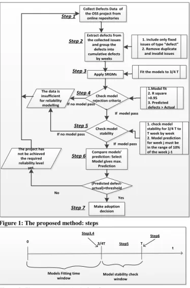
The method is defined by the following steps (see also Figure 1 and Figure 2)
1. The first step is to select the release of the OSS project of interest and collect the issues from the online repositories. There are many online repositories, such as sourceforge, apache, bugzilla etc, which contain issues and defects data of OSS projects.
2. The second step is to extract defects from the issues collected in step 1. Issues can be bugs, feature requests, improvements, or tasks. The issues need to be filtered in order to include only those issues that have been declared as a “bug” or a “defect” and exclude “enhancements,” “feature-requests,” “tasks” or “patches”. Further, only defects that were reported as closed or resolved are considered, open or reopen defects are excluded. Finally, duplicate defects must be excluded too. The defects data of the whole release interval [0, T] are grouped into cumulative defects by weeks.
3. The third step is to apply the SRGMs listed in Table 1 to the defects data obtained from step 2. The models are fitted to the defect data of 3/4T; that is represented as ‘model fitting window’ in figure 2. Fitting can be done using Non Linear Regression (NLR) techniques. NLR is a general technique to fit a curve through the data. The parameters are estimated by minimizing the sum of the squares of the distances between the data points and the regression curve. NLR is an iterative process that starts with an initial estimated value for each parameter. The iterative algorithm then gradually adjusts these parameters until they converge on the best fit so that the adjustments make virtually no difference in the sum-of-squares. A model’s parameters do not converge to the best fit if the model cannot describe the data. As a consequence the model cannot fit the data. If a curve can be fitted to the data for a model, the goodness of fit (GOF) value is evaluated based on the R2-value,
Apply SRGMs 1.Model fit 2. R square >0.95 3. Predicted defects > Actual Check model rejection criteria Check model stability 1. check model stability for 3/4 T to T week by week 2. Model prediction for week j must be in the range of 10% of the week j-1 Compare models’
prediction: Select Model gives max.
Prediction (Predicted defect-actual)=threshold Make adoption decision No
The project has not be achieved the required reliability level
yet.
Extract defects from the collected issues and group the
defects into cumulative defects
by weeks
1. include only fixed issues of type “defect” 2. Remove duplicate and invalid issues
The data is insufficient for reliability
modelling If no model pass
Yes If model pass If no model pass Step 2 Step 3 Step 4 Step 5 Step 6 Step 7 If model pass
Fit the models to 3/4 T
Figure 1: The proposed method: steps
0
Models Fitting time
window Model stability check window 3/4T Step5 Step3,4
Step6 T
t
Figure 2: The proposed method: time frames
In the expression k represents the size of the data set, m(ti) represents predicted cumulative failures and mi represents actual cumulative failures at time ti. R
2
takes a value between 0 and 1, inclusive. The closer the R2 value is to one, the better the fit. The R2-value is used for its simplicity and is motivated by the work of Gaudoin, O. et al [18], who evaluated the power of several statistical tests for GOF for a variety of reliability models. Their evaluation showed that this measure was as least as powerful as the other GOF tests analyzed. The larger the R2 value, the better the fitted model explains the variation in the data. Fitting the curves of the models estimates the value for all parameters of the fitted model and notably the expected number of total defects (‘a’ parameter).
For model fitting we use a commercial curve fitting program that uses NLR techniques for the model curve fitting. Model equations along with constraints on the model parameters are supplied to the program. The program then fits the model to the data, returns an estimate of the best fitted values for all the parameters of the models along with the GOF value, i.e. R2. We use NLR for model fitting due to the nature of collected defect data.
4. In this step models are passed through model rejection criteria. Fitted models GOF values are compared with the selected threshold value of R2. Setting a threshold for the GOF value is based on subjective judgment. One may require higher or lower values for this threshold. Our choice for setting the GOF value threshold at 0.95 is motivated by the work of Stringfellow, et al [16]. Similarly fitted models predictions are checked against the actual number of defects found. Only those fitted models whose prediction is greater than the actual number of defects are retained, because the model prediction is meaningless when it predicts a lower number of defects than the actual defects found. If one model does not pass this step, this means that the collected defects data is insufficient for reliability modeling and additional data is required.
5. In this step models are evaluated in term of prediction stability. A prediction is stable if the prediction for week j is within ±10% of the prediction for week j-1. Setting a threshold for stability is based on subjective judgment. One may require higher or lower values for this threshold. Our rationale for setting this threshold at 10% is motivated by Wood’s suggestion of using 10% as a stability threshold [19]. If no model has a stable prediction that is within the stability threshold defined, this means that the collected defects data is insufficient for reliability modeling and additional data is required.
For the purpose to check model stability the time window from 3/4T to T is used; that is represented as ‘model stability check window’ in figure 2. For instance, the model stability is checked as follows: in cumulative defects of the 3/4T, add one week defect, i.e. 3/4T+1week, then fit all the models that have passed the rejection step, to cumulative defects of 3/4T+1week, after this another week is
5
added, i.e. 3/4T+2weeks, and so on till T. A model is stable if its prediction for week j is within ±10% of the prediction for week j-1.
6. The sixth step is to select the best SRGM model. The model which gives the highest number of predicted defects among all stable models is selected. It is a conservative choice. The rationale is to select the safer model. In practice we consider suitable the models which overestimate the actual number of defects because defect fixing cost in earlier stages (i.e. before adoption of an OSS) would be less than the defects fixing cost in later stages (i.e. after the adoption of the OSS). If there is a large difference in values for the prediction between different models, one may want to either augment this analysis with other quality assessment methods, as shown in [20], or choose a subset of models based on the GOF indicator.
7. In this step, using the selected SRGM, the residual defects of the OSS are computed. In function of the number of residual defects the project manager may decide to adopt the OSS, wait some more time (i.e. wait for more defects to be found and fixed), adopt another OSS or closed source component.
V. APPLICATION OF THE METHOD
Here we apply our method to the selected seven OSS projects to show in practice how it works. The next section A describes the OSS projects selected, and section B gives the results.
A. OSS Projects Selected
Many open source projects are undergoing development and each project produces a lot of data sets. Therefore, it is important to select representative open source projects for the validation of a method. We selected seven projects of different nature having large and well-organized communities; Apache, GNOME, C++ Standard Library, JUDDI, HTTP Server, XML Beans, and Enterprise Social Messaging Environment (ESME). For Apache and GNOME the s defects data were available in literature. We took defect data about three different releases of Apache and three different releases of GNOME published by Xiang Li et al [9]. The first two steps of our method do not apply to these datasets because these datasets were already grouped into cumulative defects by week from the corresponding release dates.
Besides GNOME and Apache, we identified five notable and active open source projects from apache.org (https://issues.apache.org/). These projects are C++ Standard Library, JUDDI, HTTP Server, XML Beans, and Enterprise Social Messaging Environment (ESME). All these projects are considered stable in production. The 66%, 95%, 68%, 64% and 82% of the reported issues in these projects respectively, have been fixed and closed. We
collected defect data of the selected projects from apache.org using JIRA. JIRA is a commercial issue tracker. Issues can be bugs, feature requests, improvements, or tasks. JIRA track bugs and tasks, link issues to related source code, plan agile development, monitor activity, report on project status.
We downloaded all the issues about three (3) releases of C++ Standard Library, three (3) releases of JUDDI, two (2) releases of HTTP Server, four (4) releases of XML Beans and three (3) releases of ESME. The tracking software records all the information regarding each issue, among which following are the more useful attributes that we used for filtration of the downloaded issues:
Project: It contains the project name;
Key: The unique identity of each issue.
Summary: It gives a comprehensive description of the issue.
Issue Type: Describes type of the issue, which may be bug, task, improvement, or new feature request.
Status: Describes current status of the issue. It may be resolved, closed, open or reopened.
Resolution: It shows resolution of the issue, which may be fixed, duplicate, or invalid.
Created: Shows the created date and time of the issue.
Updated: Shows the updated/fixing date and time of the issue.
Affected Versions: It gives the affected releases/versions of the project which contain the issue.
According to the step 2 of our method we filtered all the collected issues. We included only those issues whose status was “closed” or “resolved”. We filtered all the issues in order to collect only issues that have been declared “defect” or “bug” as in [10]. The refined data is grouped into cumulative defects by weeks on the basis of created data. Due to space limitation full defect data set of each release is available online2.
B. Results
Due to space limitations we show here (Table 2) the results of the application of the method to one release of one project. The results for all releases of all projects are also available online3.
The method has been applied using, for each version of each project, 2/3rds of the time window available, and of the corresponding defects. The remaining 1/3 is used for validation, as explained in section VI.
Let’s start by discussing the application of the method to GNOME release 2.0 (Table 2). The time interval available
2 http://softeng.polito.it/najeeb/IEEE/Datasets.pdf 3 http://softeng.polito.it/najeeb/IEEE/Remaining_results.pdf
release Pred. R2 Pred. R2 Pred. R2 Pred. R2 Pred. R2 Pred. R2 Pred. R2 Pred. R2 12 58 945 0.9806 66 0.9859 926 0.9806 68 0.974 59 0.9937 1743 0.9806 73 0.9889 105 0.9819 13 58 446D 0.9836 791D 0.9836 455D 0.9836 71S 0.9781 62S 0.9937 883D 0.9836 74 0.9909 100 0.9852 14 66 78 0.9764 69 0.9879 84D 0.9891 202D 0.9866 15 72 86 0.9747 78 0.9844 16 74 90 0.9772 83 0.986
Project Release PRE of the model
Musa Inf. Goel Delay. Log. Yama. Gomp. Gener.
Best model on PRE Best model selected by
proposed method
GNOME V2.0 0.19 0.08 0.18 0.01 -0.02 0.18 0.05 -0.85 Delayed Delayed
V2.2 0.09 -0.07 0.00 -0.11 -0.10 0.00 -0.10 -0.47 Goel, Yamada Goel V2.4 0.14 0.01 0.04 -0.03 -0.02 0.03 -0.01 -0.28 Inflection, Gompertz Inflection Apache 2.0.35 0.17 0.07 0.12 -0.01 -0.01 0.12 0.03 -0.53 Delayed, Logistic Gompertz
2.0.36 0.18 0.03 0.09 0.01 0.01 0.09 0.01 0.01 Delay, Log, Gompertz, General. Generalized 2.0.39 0.15 0.00 0.00 -0.02 -0.02 0.02 -0.01 0.00 Inflection, Goel, General. Goel C++
Stand. Lib
4.1.3 -0.22 -0.25 -0.39 -0.52 -0.45 -0.34 -0.41 -0.31 Musa Inflection
4.2.3 -0.01 -0.05 -0.12 -0.20 -0.07 -0.09 -0.03 0.06 Musa Gompertz
5.0.0 -0.28 -0.16 -0.66 -0.98 -0.92 -0.16 -0.83 -0.16 Inflection, Yamada, General. Yamada JUDDI 3.0 0.00 0.24 0.00 0.00 0.26 0.00 0.00 0.13 Musa, Goel, Delay, Yama, Gomp Delayed 3.0.1 -0.02 -0.32 -0.10 -0.02 -0.05 -0.10 -0.27 -0.29 Musa, Delayed Delayed 3.0.4 -0.30 -0.33 -0.27 -0.72 -0.67 -0.34 -0.59 -0.33 Goel Goel HTTP
Server
3.2.7 0.04 -0.10 0.02 -0.18 -0.16 -0.05 -0.11 -0.05 Goel Goel 3.2.10 0.23 0.22 0.23 0.01 0.01 0.23 0.13 0.23 Delayed, Logistic Logistic XML
Beans
2.0 0.17 0.02 0.17 -0.02 -0.14 0.17 0.01 0.07 Gompertz Delayed & Gompertz 2.2 -0.04 0.04 -0.04 -0.29 0.01 -0.03 0.11 -0.02 Logistic Logistic
2.3 0.00 0.05 0.00 -0.25 0.00 0.00 0.01 0.00 Musa, Goel, Log, Yama, General. Logistic 2.4 0.24 -0.12 0.24 0.06 -0.16 0.24 0.06 -0.11 Delayed, Gompertz Gompertz ESME 1.1 -0.03 -0.23 -0.03 -0.32 -0.34 -0.14 -0.29 -0.23 Musa, Goel Goel
1.2 -0.26 -0.33 -0.41 -0.57 -0. 09 -0.37 -0.09 -0.16 Logistic, Gompertz Gompertz
1.3 0.18 0.07 0.07 -0.02 -0.02 0.08 -0.02 0.07 Delayed, Logistic, Gompertz Inflection, Goel, Generalized
is 24 weeks. As said we use 2/3 of this time frame for model selection, or 16 weeks. Of these, we use the last 1 /4 for model stability check, or weeks 12 to 16. Table 2 contains a row for each week, from 12 to 16. For each week the table shows, in the columns, from left to right: the number of actual cumulative defects found in that week, and, for each of the eight SRGMs, the number of total defects predicted, and the R2 value.
Each of the eight models is fitted each week. When a model fails the stability check it is rejected (this is indicated by letter ‘R’). The week a model stabilizes is indicated by an ‘S’. If a model becomes unstable after being stable, this is indicated by a ‘D’. The model selected by the method is underlined.
In Table 2 GOF values of all the models show that all the models perform very well in terms of fitting and pass the rejection criteria but their predictions are different. Musa, Inflection, Goel, and Yamada destabilize at week 13 whereas Gompertz and Generalized destabilize at week 14. All these models overestimate by a very large amount. From Table 2 it is also clear that the Delayed S-shaped and Logistic models stabilize first at week 13 and remain stable up to week 16 (i.e. throughout the whole stability check window). The Delayed S-Shaped and Logistic models predict the number of defects at week 16 as 90 and 83
respectively. Since the Delayed S-shaped model predicts more residual defects than Logistic, it is selected.
VI. VALIDATION
We apply our method to 2/3 of each release interval defect data to select the best model. The remaining defect data of each release are used for validation. The choice of 2/3 release interval for the estimation of model parameters was motivated by Wood’s suggestion that the model parameters do not become stable until about 60% of the way through the test [19].
As a measure to validate the prediction capability of a model we use the PRE (Prediction Relative Error) indicator.
Where Predicted is the total number of defects predicted by a model, as fitted at 2/3 of the time interval available, and
Actual number of defects is the number of defects at the end of the time interval.
For each release and each project we compute PRE for each model, and rank the models accordingly. The model with Table 3: Best predictor model selected by our method Vs best predictor selected on prediction PRE
7
minimum PRE is considered the best predictor model for that release.
Table 3 shows the validation results: for each project and each release the best model on PRE and the best model according to the method. We observe that 17 out of 21 times, the model selected by the method corresponds to the best model. In the remaining four cases the best model has a negative PRE, and for this reason was rejected by the method. However, in these four cases the model selected by the method is the one with the lowest positive PRE (the lowest negative for C++ 4.2.3). This means that in these four cases the method selects the second best model.
VII. THREATS TO VALIDITY
The first construct threat comes from the issues data sets used. We use data sets produced by others, so we have no control on the quality of the issues collected and reported. Issues could be missing; others could have been mis-reported, either on time or on content. Overall we have tried to reduce this threat by selecting established Open Source projects and communities. Most of the datasets we used have also been used in other similar works.
Still on construct validity, we have considered each release of a project as a separate project, independent of others. This choice is in line with [2, 10, 19, 20]. As a cross validation of this independence it should be noted that different versions of the same project are best fitted by different SRGMs.
The time span covered by the datasets of projects, and project versions, is quite different. We assume this is not critical, especially because we do not compare project versions, but we consider each project version independently.
We recognize one external threat to validity. We have evaluated our method on 21 projects. This is one of the largest datasets in literature but we cannot generalize the results to all projects. In particular the method could just be not applicable to a project because curve fitting, satisfaction of GOF or stability thresholds could fail. In these cases the thresholds can be changed.
VIII. DISCUSSION
The results of the empirical validation show that the proposed method selects the best or second best model, in terms of better precision in the estimation of the residuals,, in all datasets. Beyond these promising results, some observations, derived both from the results and the application itself of the method, are worthy to be discussed. We begin our discussion from the observations derived from the results.
Firstly, no model is clearly superior to others. In fact, in the 21 data sets no model ranks as the best one in more than a few cases, and each of the eight models is the best one at least once. This is in line with the fact that also related work did not converge on the goodness of one reliability model, and further supports the need for a methodology which enables to select the best SRGM model for a given project.
Our results show also that different releases of the same project are each fitted by different models. This is in line with the assumption –common in the related literature - that releases should be considered as independent projects. A possible explanation is that only the history of defects and not any other project characteristic counts for the model selection. The factors that determine the history of defects, although investigated since decades, are not yet fully understood. The cause for high number of defects can reside in the product characteristics (measured with structural metrics like code complexity, coupling, etc.), or in the intrinsic difficulties of the domain, or in people’s skill. Also processes and organization might indirectly have an effect on the external quality of a software product.
A few other considerations derive from the application of the method.
One of them is that most of the time models are rejected due to prediction instability instead of GOF value. This could be explained by the fact that not enough defect data is available. The method overcomes this obstacle with the wide number of models available, however in a real scenario this could be a problem: further work could investigate what is the minimum amount of defect data needed for the selection of a SRGM. The second observation regards S-Shaped models: they outperform concave ones in 14 out of 21 cases, which also confirm the results of our previous studies [10]. S-Shaped models are better probably because initially the community of end-users and reviewers of the open source projects do not react promptly to a new release. This is modeled by the learning phase included in the S-Shaped models.
There is more than one model that fits the defect data after 5 weeks (in terms of the method, at least a model passes step 4 after 5 weeks). So 5 weeks could be the suggested as an initial rule of thumb for the delay from release before doing any analysis about reliability.
Finally, the method we propose sets some parameters: the GOF minimal threshold for fitting (0.95), the stability threshold (10%), the time frames (last 1/4 of defect data for fitting and stability check). These parameters were set using suggestions from the literature and seem to perform well. Sensitivity analysis on the threshold was out of the scope of our evaluation; however it could be source of inspiration for further work.
IX. CONCLUSIONS
The goal of this work was to support practitioners in characterizing the reliability (in terms of residual defects) of an OSS component or application, to help a project manager in deciding whether using the OSS or not in a project. To achieve the goal we proposed a pragmatic approach, which selects best model both on its fitting capability, and on the stability of its prediction over time. The model selected with our proposed method, among several alternative models predicts very precisely the residual defects of an OSS. We believe that the key contribution of this work lies in the systematic approach (eight SRGM models have been
tool to automate the method.
References
[1] IEEE Std 1633-2008 IEEE Recommended Practice in Software Reliability.
[2] Kapil Sharma, et al, “Selection of Optimal Software Reliability Growth Models Using a Distance Based Method”, IEEE Transactions on Reliability, Vol. 59, No. 2, June 2010.
[3] J.D. Musa, A. Iannino, and K. Okumoto, Software Reliability, Measurement, Prediction and Application. McGraw-Hill, 1987. [4] G. H. Schick and R. W. Wolverton, “An analysis of competing
software reliability models,” IEEE Trans. Software Engineering, pp. 104–120, March 1978.
[5] A. N. Sukert, “Empirical validation of three software errors predictions models,” IEEE Transaction on Reliability, pp. 199–205, August 1979.
[6] S. Brocklehurst, P. Y. Chan, B. Littlewood, and J. Snell, “Recalibrating software reliability models,” IEEE Trans. Softw. Engineering, vol. SE-16, no. 4, pp. 458–470, April 1990.
[7] A. L Goel, “Software reliability models: assumption, limitations, and applicability,” IEEE Transaction on Software Engineering, pp. 1411–1423, December 1985.
[8] Abdel-Ghaly, P.Y. Chan, and B. Littlewood, “Evaluation of competing software reliability predictions,” IEEE Trans. Softw. Engineering, vol. SE-12, no. 12, pp. 950–967, September 1986. [9] Xiang Li et al. 2011. Reliability analysis and optimal
release-updating for open source software. Information and Software Technology 53 (2011) 929–936.
[10] Najeeb ullah, Maurizio Morisio. An Empirical Study of Reliability Growth of Open versus Closed Source Software through Software Reliability Growth Models. Proceeding of APSEC 2012.
[11] Basili, et al, "The Goal Question Metric Method", in Encyclopedia of Software Engineering, Wiley, 1994.
[12] M.R. Lyu, Handbook of Software Reliability Engineering. McGraw Hill, 1996.
[13] J. D. Musa and K. Okumoto, “A logarithmic Poisson execution time model for software reliability measurement,” in Conf. Proc. 7th International Conf. on Softw. Engineering, 1983, pp. 230–237. [14] M. Xie, Software Reliability Modeling. World Scientific Publishing,
1991.
[15] H. Pham, “Software reliability and cost models: perspectives, comparison and practice,” European J. of Operational Research, vol. 149, pp. 475–489, 2003.
[16] Stringfellow, et al. An empirical method for selecting software reliability growth models. Empirical Software Engineering, Journal. Page 319-343, 2002.
[17] K. C. Chiu, Y. S. Huang, and T. Z. Lee, “A study of software reliability growth from the perspective of learning effects,” Reliability Engineering and System Safety, pp. 1410–1421, 2008. [18] Gaudoin, O., Xie, M., and Yang, B. A simple goodness-of-fit test for
the power-law process, based on the Duane plot. IEEE Transactions on Reliability. 2002.
[19] Wood, Alan, “Software-reliability growth model: primary-failures generate secondary-faults under imperfect debugging and. IEEE Transactions on Reliability, 43, 3, 408 (September 1994).” [20] Stringfellow, C. 2000. An integrated method for improving testing
effectiveness and efficiency. PhD Dissertation, Colorado State University.
[21] Neha Miglani and Poonam Rana, Ranking of Software Reliability Growth Models using Greedy Approach, Global Journal of Business Management and Information Technology, Vol 1. No 11, 2011 [22] Mohd. Anjum, Md. Asraful Haque, Nesar Ahmad, Analysis and
Ranking of Software Reliability Models Based on Weighted Criteria Value, I.J. Information Technology and Computer Science, 2013, 02
Politecnico di Torino. The main goal of his doctoral activities is to study reliability of open source software, the factors affecting the reliability trend of OSS. His recent interests are focused on software reliability models. The methodology he uses is that one of the empirical software engineering. He received a B.Sc. degree in computer science for university of Peshawar, Pakistan and a specializing master degree in Computer Engineering from Politecnico di Torino. He has research interests in software reliability, software process improvement and empirical software engineering.
Maurizio Morisio is Full Professor at Dept. of Control and Computer Engineering of the Politecnico di Torino, where he leads the software engineering group. In 1998-2000 he spent two years at the University of Maryland at College Park, working with the Experimental Software Engineering Group led by Vic Basili. From September 1998 to June 2000 he was on the board of directors of the SEL (Software Engineering Laboratory), a consortium among NASA Goddard Space Flight Center, the University of Maryland and Computer Science Corporation, with the aim of improving software practices at NASA and CSC. He got a Ph.D. in Software Engineering and a M.Sc. in Electronic Engineering from Politecnico di Torino. He has published more than 70 papers in international journals and conferences and three books. He is associate editor in chief of IEEE Software and Empirical Software Engineering Journal since 2008.
Antonio Vetrò is a postdoctoral research fellow at Technische Universität München, Germany. He has completed his Ph.D degree at Politecnico di Torino, Italy. The main goal of his doctoral activities were to evaluate how automatic static analysis can be used to improve specific attributes of software quality. He is specialized on empirical methodologies and analyses of process and product data. He has been Junior scientist at Fraunhofer Center for Experimental Software Engineering at College Park, MD, USA, in 2011. He received a B.Sc. in Business Organization Engineering and a M.Sc. in Computer Engineering from Politecnico di Torino.