Learning Structured Models for Segmentation of 2D
and 3D Imagery
Aur´elien Lucchi
1Pablo M´arquez-Neila
2Carlos Becker
2Yunpeng Li
2Kevin Smith
3Graham Knott
4Pascal Fua
21
Department of Computer Science, ETH, Z¨urich, Switzerland
2Computer Vision Laboratory, EPFL, Lausanne, Switzerland
3
Biozentrum, University of Basel, Switzerland
4
Interdisciplinary Center for Electron Microscopy, EPFL, Lausanne, Switzerland
Index Terms—Image processing, computer vision, electron microscopy, image segmentation, kernel methods, mitochondria, statistical machine learning, structured prediction, segmentation, superpixels, supervoxels.
Abstract—Efficient and accurate segmentation of cellular structures in microscopic data is an essential task in medical imaging. Many state-of-the-art approaches to image segmentation use structured models whose parameters must be carefully chosen for optimal performance. A popular choice is to learn them using a large-margin framework and more specifically structured support vector machines (SSVM). Although SSVMs are appealing, they suffer from certain limitations. First, they are restricted in practice to linear kernels because the more powerful non-linear kernels cause the learning to become prohibitively expensive. Second, they require iteratively finding the most violated constraints, which is often intractable for the loopy graphical models used in image segmentation. This requires approximation that can lead to reduced quality of learning.
In this article, we propose three novel techniques to overcome these limitations. We first introduce a method to “kernelize” the features so that a linear SSVM framework can leverage the power of non-linear kernels without incurring much additional computational cost. Moreover, we employ a working set of constraints to increase the reliability of approximate subgradient methods and introduce a new way to select a suitable step size at each iteration.
We demonstrate the strength of our approach on both 2D and 3D electron microscopic (EM) image data and show consistent performance improvement over state-of-the-art approaches.
I. INTRODUCTION
Semantic segmentation of 2D images and 3D image stacks is a fundamental medical image processing task. Graphical models, such as conditional random fields (CRF) [6], [25] are widely used for this purpose because they capture the inter-dependency between nearby pixels by minimizing an energy function, or equivalently maximizing a score function, which depends on both local data evidence and spatial consistency of the output. These models, however, typically involve a large number of parameters that must be carefully chosen to achieve good performance and learning them efficiently is
Copyright (c) 2014 IEEE. Personal use of this material is permitted. However, permission to use this material for any other purposes must be obtained from the IEEE by sending a request to [email protected].
This work was supported in part by the EU ERC Grant MicroNano.
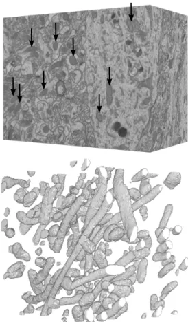
Fig. 1. A nearly isotropic stack of neural tissue acquired from the CA1 hippocampus using EM microscopy.Top.This stack is made of 10652048×
1536 slices and its resolution is 5 nanometer in all three directions. This
represents more than 3 billion voxels for a volume whose largest dimension is in the order of 10µm. The black arrows point towards mitochondria, which we use to train our CRF-based segmentation algorithm.Bottom.3D rendering of the mitochondria found in a1024×1024×1024subvolume.
a challenging task. It is particularly daunting when dealing with large datasets such as the one depicted by Fig. 1, which modern imaging devices can now routinely produce.
The maximum-margin framework [52] has gained much popularity in recent years as a means to do this. As an
alternative to maximum likelihood and maximuma posteriori
learning, it makes unnecessary the difficult task of estimating the partition function and can be used in conjunction with many different performance metrics. The structured support vector machine (SSVM) [55] is a particularly successful variant of this approach, in which the learning objective is to minimize a regularized hinge loss caused by the violation of a set of soft margin constraints.
Although SSVMs have made the learning task easier than before, they are, nevertheless, not without their limitations. Though highly efficient when the CRF energy function is linear, they can become prohibitively expensive when non-linear kernels are involved, especially in the case of kernels computed over the graph nodes. This is because the number of kernel evaluations required, and hence the training time, scales quadratically with respect to the number of pixels or nodes in the CRF. This quickly makes the problem unmanageable for even moderate size datasets. Thus, it is usually impractical to directly apply non-linear kernels in an SSVM framework, even though they are often more powerful than their linear counterpart.
Moreover, optimizing the SSVM objective function can be challenging regardless of the linearity of the CRF energy. It is usually done iteratively using either the SSVM cutting plane algorithm [55] or by solving the equivalent unconstrained optimization problem using subgradient based methods [40], [32], [35], [58]. Either way, the most violated constraint
must be found at every iteration. This means finding the labeling that maximizes the margin-sensitive hinge loss [55] and yields a valid cutting plane or true subgradient of the objective. This, however, is intractable for the loopy graphical models used for image segmentation. Although approximate maximizers obtained by approximate inference, such as belief propagation [34] and graph cuts [7] can be used as substi-tutes, the approximation are usually so imprecise that they adversely impact the learning process. In the worst case, an unsatisfactory constraint can cause the cutting plane algorithm to prematurely terminate if it does not have a higher hinge loss than previous constraints. It can also induce erratic behavior in subgradient-based methods when the implied descent direction is too far away from any true subgradient.
Another difficulty with subgradient-based methods is that they rely heavily on choosing an appropriatestep size, that is, the distance by which to advance in the negative subgradient direction at each iteration. Many algorithms rely on preset, non-adaptive, and usually decreasing sequences of values. In theory, they provide theoretical asymptotic convergence guarantees. However, in practice, the inflexible nature of fixed-sequence step sizes often causes unsuitable values to be used, which negatively impacts the quality of the solutions obtained in finite time.
These phenomena make the learning process more suscep-tible to failure and limit the predictive power of the model. In this work, we develop and combine three new techniques to overcome these limitations.
• Kernelized Features. We formulate a two-stage training procedure that lets us combine the strength of SSVM and non-linear kernels in an efficient manner. To this end,
we first use a regular non-linear non-structured SVM to create a set of support vectors from the training data. We then use it to transform our initial feature vectors intokernelized features, that is, the kernel product of the input feature vectors and the support vectors. We then train a linear SSVM using the kernelized features instead of the original ones, which lets us leverage the power of non-linear kernels without the computational burden of non-linear SSVM training.
• Working Set Approach to Computing Subgradients. We introduce an approximate subgradient method that uses a working set of constraints to make learning more robust. It is specifically designed to minimize the margin-sensitive hinge loss in the SSVM formulation when the most violated constraints and hence the resulting subgradients are not exact. We use a whole working set of constraints, unlike existing subgradient approaches that only consider the most recent one. This makes our method more reliable even when the subgradients estimated from individual constraints are noisy. In cases where fast training is important, it also allows us to estimate the subgradients by randomly sampling label-ings instead of explicitly looking for the most violated constraints. This speeds up training at only a small loss in classification accuracy.
• Adaptive Step Size Selection. We propose a new ap-proach to setting the step sizes adaptively at each iteration by exploiting knowledge about the objective function that we have accumulated during earlier iterations. More specifically, we use the working set of previously found constraints to compute the next step size. Our key ob-servation is that previous constraints can be used to calculate a lower bound on the learning objective, which is informative for guiding the optimization. Our method preserves the asymptotic convergence properties of the sub-gradient descent (SGD), has a low computational overhead, and consistently yields improved solutions. We introduced the first two techniques separately in [29] and [28] and the third one is new. We show that these three techniques can be combined and demonstrate that the resulting approach boosts CRF performance on both 2D and 3D datasets.
The remainder of the article is organized as follows. We discuss prior work in Section II and provide the background on the large-margin framework and corresponding learning techniques in Section III. Our three contributions are intro-duced in the three following sections, our kernelized features in Section IV, our working set approach in Section V and our adaptive step size selection in Section VI. We present our experimental results in Section VII.
II. RELATED WORK
For tasks such as segmentation, the labels of neighbor-ing pixels tend to be highly correlated and modelneighbor-ing such correlations is often key to achieving high accuracy. As a result, structured prediction has emerged as a highly useful framework for tackling this class of problems. In this section,
we first briefly review existing versions of this framework and then discuss current approaches to learn their parameters and adjusting step-sizes during the optimization.
A. Structured Prediction and Non-linear Kernels
Structured prediction methods such as conditional random fields (CRFs) [25] have been widely applied to problems with structured outputs. While traditional classifiers, such as deci-sion trees and SVMs independently map each data instance to a single label, structured prediction methods take into account the correlations between labels. This is critical for tasks such as image segmentation, where such correlations are strong between nearby pixels. Learning CRF models using large-margin methods has rapidly gained popularity in recent years, largely due to the fact that they are more objective-driven and do not involve the daunting partition function that can render maximum-likelihood approaches intractable in CRFs with loopy graph structures. Compared with earlier approaches including the max-margin Markov network [52], the structured support vector machine (SSVM) [55] is especially appealing because of its expressiveness and flexibility, and has since been successfully applied to many computer vision tasks, such as in [50], [36], [27], among many others.
SSVMs, however, require the CRF energy function to be expressible in a linear form, which in turn places the same restriction on all the unary and spatial terms due to the additive nature of CRF energies. While, in principle, the linear function can be defined in some high dimensional or possibly infinite-dimensional space, reproducing this kernel Hilbert space through the use of non-linear kernels is often infeasible in practice given that the number of kernel evaluations grows quadratically with the model size and must be optimized in the dual space. Though SSVM learning techniques based on sampled cuts [59], [44] have alleviated this problem to some extent, they sacrifice performance for speed. Even with this trade-off, they are still much slower than linear SSVMs [59]. Moreover, earlier implementations of these techniques were intended for use in conjunction with the cutting-plane method to speed up training of regular non-linear SVMs. This results in amultivariateoutput space in the SSVM formulation, which is analogous to a CRF without edges, and thus considerably simpler than the models typically used for image segmentation. Kernel Approximation is another way to improve SSVM training efficiency by seeking a lower, finite-dimensional rep-resentation of the kernel-induced feature map that lies in a higher or infinite dimensional space. This can be achieved by random sampling from the typically infinite-dimensional feature map [39], [3] whose analytical form can be obtained using Fourier analysis when the kernel is homogeneous or stationary [56]. While promising results have been shown for specific additive kernels [31], [56], it is less clear how this approach generalizes to non-additive kernels, such as the Gaussian RBF that is more difficult to approximate. Alternatively, the locally linear SVM [24] can be used to simulate a non-linear decision boundary. However, this does not yield a globally linear function and, thus, does not fit into the SSVM framework. Moreover kernel approximation
typically introduces additional tuning parameters such as the number of samples, which often present a performance-speed trade-off for which there are no well-defined tuning criteria.
Finally, it is worth pointing out the difference between our approach and the recently proposedstructural kernels, which also perform structured prediction using non-linear kernels, but in a very different setting. In [44], [4], the kernels are defined on the overall output space, that is, the entire CRF, to exploit image-level “structural” information such as shape and color. While this serves to bias local labels and is useful for segmenting large dominant objects from the background, it often requires training data that completely characterizes the possible object configurations, such as binary masks. Multiple objects or objects whose pose are not represented in the trained model will cause the approach to fail. Our approach, on the other hand, uses regular kernels defined as products between a set of support vectors and the feature vectors extracted from individual nodes. This has the effect of making it more “local”, and thus not susceptible to such failures.
B. Learning methods for structured models
Maximum margin learning of CRFs was first formulated in the max-margin Markov networks (M3N) [52], whose objec-tive is to minimize a margin-sensiobjec-tive hinge loss between the ground-truth labeling and all other labelings for each training example. This is especially appealing for learning CRFs with loopy structures, due to its more objective-driven nature and the fact that it completely bypasses the partition function, which presents a major challenge to maximum likelihood based approaches. Nevertheless, the number of constraints in the resulting quadratic program (QP) is exponential in the size of the graph, making the optimization a non-trivial problem. In M3N this is handled by rewriting the QP dual in terms of a polynomial number of marginal variables, which can then be solved by a coordinate descent method analogous to the sequential minimal optimization (SMO) [37]. However, solving such a QP is not tractable for loopy CRFs with high tree widths that are often needed in many computer vision tasks. In fact, even solving it approximately can become overwhelmingly expensive on large graphs.
Structured SVMs (SSVM) [55] optimize the same kind of objective as M3N, while allowing for a more general class of loss functions. It employs a cutting plane algorithm to itera-tively solve a series of increasingly larger QPs, which makes learning more scalable. However, the cutting plane algorithm requires the computation of the most violated constraints, namely the labeling that maximizes the hinge loss [55]. This involves performing theloss augmented inference[51], which is intractable on loopy CRFs. Though approximate constraints can be used [14], they make the cutting plane algorithm susceptible to premature termination and, in the worst case, can lead to catastrophic failure. This problem is considered in [50], which limits the optimization to a smaller parameter space where exact inference can be performed with graph cuts. However the addition of the hard submodularity constraints makes the resulting QP more expensive to solve, especially when the dimensionality of the feature space is also high.
In order to speed up the computation, a caching strategy was proposed in [19]. Instead of performing the loss augmented inference at every iteration, the algorithm first tries to construct a sufficiently violated constraint from the cache. While its use of a cache bears certain apparent similarity to the working set method described in this article, the goal of caching in [19] is to decrease the number of calls to the separation oracle while our approach aims at increasing the robustness of approximate subgradient methods.
An alternative to solving the quadratic program determin-istically is to employ a stochastic gradient or subgradient method. This class of algorithms has been studied extensively for non-structured prediction problems [46]. In the context of structured prediction, learning can be achieved by finding a convex-concave saddle-point and solving it with a dual extra-gradient method [53]. In [40] max-margin learning is solved as an unconstrained optimization problem and subgradients are used to approximate the gradient in the resulting non-differentiable problem. This method trades optimality for a lower complexity, making it more suitable for large-scale problems. The approach of [32] proposes a perceptron-like algorithm based on an update whose expectation is close to the gradient of the true expected loss. However, the soundness of these methods heavily depends on the assumption that a valid subgradient is obtained at each iteration. Hence they become much less reliable when the subgradients are noisy due to inexact inference, as is the case for loopy CRFs.
The recently proposed SampleRank [57] avoids performing inference altogether during learning. Instead, it samples label-ings at random using Markov chain Monte Carlo (MCMC). At each step, parameters are updated with respect to a pair of sampled labelings. Hence, unlike our method, it solves a problem that is substantially different from the original max-margin formulation. Though achieving notable speed improve-ment, the method does not in fact optimize the actual hinge loss but rather a loose upper bound on it.
C. Adaptive step-size
The performance of SGD largely depends on the ability to choose appropriate step sizes. They often have to be carefully tuned for the specific data at hand because inappropriate choices can easily lead to inferior solutions and slow con-vergence.
Several strategies for automatically choosing them are dis-cussed in [5]. Most methods use preset step size sequences that are determined offlineand are not adaptive [42], [46]. Typical choices include simple diminishing sequences and Polyak step sizes [38], the latter being suitable only when the optimal function value is known or can be estimated, and the evaluation of the objective function is possible andeasy.
Nevertheless, a number of adaptive or “online” schemes have been studied in the literature and typically involve a line search to decide how far to move along a given descent direction. Exact searches are usually expensive and tend to be replaced by approximate searches methods based on Wolfe’s sufficient conditions for convergence, where step sizes depend on the current point and the current search direction. Gain
adaptation methods such as stochastic meta-descent (SMD) also accelerate convergence by using second-order information to adjust the gradient step sizes [43], but require being able to efficiently compute the Hessian. Another online approach is the margin infused relaxed algorithm (MIRA) [10] that uses the notion of margin to update its solution. It attempts to keep the current solution and the solution at the next iteration as close as possible while fully satisfying the margin requirement. Choosing step sizes adaptively for subgradient based struc-tured learning is also gaining attention. For example, the MIRA algorithm [10] was extended to structured outputs in [11]. Recently a stochastic coordinate ascent algorithm for solving structured SVM based on the Frank-Wolfe algorithm was developed in [23]. This approach automatically computes the step sizes in closed-form that corresponds to the result of line search in the dual space. The bundle approach to structured prediction [15], [26], [54] generalizes the cutting plane one by estimating a piecewise linear lower bound from cutting planes computed as objective function subgradients. A proximal function or a regularizer is commonly used to prevent over-large iteration steps. In fact, the bundle method of [54] generalizes SSVM [55] when the objective function includes a quadratic regularizer. Like both the cutting plane and bundle methods, ours exploits all the previously accu-mulated constraints. However, unlike these methods, it only requires a 1D line search in the subgradient direction, which can be efficiently done. Note that the soundness of most of the aforementioned subgradient methods depends heavily on the assumption that a valid subgradient is obtained at each iteration. Hence they become much less reliable when the subgradients are noisy due to inexact inference, as is the case for loopy CRFs. Our method is not exempt from this problem but we found empirically that using a working set increases the reliability of our subgradients.
III. MAX-MARGINLEARNING OFCRFS
In this section, we begin by describing the standard CRF model [25], [49] for segmentation. We then discuss how to learn its parameters within the SSVM framework, with specific attention to expressing the CRF model in the required linear form for effective learning. We will use it in Sec. IV in conjunction with our kernelized features, thus enabling us to leverage the power of non-linear kernels while the SSVM remains linear. In Section V-B, we will introduce our approach to computing the subgradients required to learn its parameters.
A. CRF for Image Segmentation
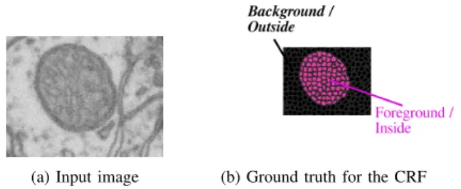
As a standard preprocessing step, we first perform a prelim-inary over-segmentation of our input image into superpixels or supervoxels [1], such as those depicted by Fig. 2. The CRF G= (V,E)is thus defined so that each nodei∈ Vcorresponds to a superpixel and there is an edge (i, j) ∈ E between two nodesiandj if the corresponding superpixels are adjacent in
the image. Let X = {xi}i∈V be an input example, such as the image or features associated to it and Y ={yi}i∈V the corresponding labeling of the CRF which assigns a class label
(a) Input image (b) Ground truth for the CRF
Fig. 2. The input image (a slice through a 3D volume) is shown in (a). Figure (b) shows the ground truth labeling of the CRF used in our method. The pink and black colors correspond to the foreground and background classes while the gray contours are the boundaries of the SLIC supervoxels.
The score function associated with the CRF can then be written as Sw(X, Y) = X i∈V Di(xi, yi) + X (i,j)∈E Vij(yi, yj), (1)
whereDi is the unary data term andVij is the pairwise spatial
term.
BothDi andVij depend on the observed data and the CRF
parametersw, in addition to the labelingY. The negated score
is also commonly referred to as the “energy” in the literature and we will use the two terms interchangeably. The inferred optimal labeling is simply the one that minimizes it, that is,
Y∗= arg max
Y∈Y
Sw(X, Y), (2)
where Y denotes the set of all possible labelings. In the remainder of this section, we will omit the input X, a
constant with respect to the maximization in Eq. 2, from the notation Sw(X, Y) for the sake of conciseness. While
the exact minimization of the score function is generally intractable on loopy CRFs, good approximate solutions can be found efficiently using techniques such as graph cuts [9] and belief propagation [34]. In our case, we use graph cuts when the score function is submodular [22] and belief propagation otherwise.
B. Discriminative Learning
Discriminative learning uses the labeled training data to learn the CRF parameters so that the inferred labeling of the CRF is “close” to that of the ground truth, defined as yielding a lowloss. More specifically, given a set ofNtraining examples
D = ((X1, Y1), . . . ,(XN, YN)) whereXi ∈ X is an input example and Yi ∈ Y is the associated labeling, the learning task consists in finding model parametersw that achieve low
empirical loss subject to some regularization. In other words, we seek w∗ = arg min w L(D,w) = arg min w 1 N X (Xn,Yn)∈D l(Xn, Yn,w) +R(w),(3)
where R(w) is the regularizer (such as the L2 norm of w) that helps prevent overfitting and l is the surrogate loss
function, a quantity that is usually related to and often defines an upper bound on the training error. Note that the definition of the surrogate lossldepends on the score functionSw, since
the goal of learning is to make the maximizer ofSwa desirable
output for the given input. The most common choice of l is
the hinge loss, as used in [52], [55] and defined as
l(Yn, Y,w) = [Sw(Y) + ∆(Yn, Y)−Sw(Yn)]+, (4) where [v]+ = max(0, v) and the task loss ∆ measures the closeness of any inferred labeling Y to the ground truth
labelingYn.
C. Max-margin Formulation
The max-margin approach is a specific instance of discrim-inative learning, where parameter learning is formulated as a quadratic program (QP) with soft margin constraints [55]
min w,ξ≥0 λ 2||w|| 2 + 1 N N X n=1 ξn (5) s.t. ∀n:Sw(Yn)≥ max Y∈Yn (Sw(Y) + ∆(Yn, Y))−ξn,
whereYn is the set of all possible labelings for examplen, the
constantC controls the trade-off between margin and training
error.
The QP can be converted to an unconstrained optimization problem by incorporating the soft constraints directly into the objective function, yielding
min w L(w) = (6) min w λ 2 ||w|| 2 + 1 N N X n=1 [Sw(Y∗) + ∆(Yn, Y∗)−Sw(Yn)]+, where Y∗= arg max Y∈Yn (Sw(Y) + ∆(Yn, Y)) (7)
is the most violated constraint of all possible labelings for example ngiven current parametersw.
Finding the optimal labelingY∗ as described in Eq. 7 is a key challenge namedloss-augmented inference.
D. Linearizing the CRF Score Function
Since the SSVM operates by solving a quadratic program (QP), all the constraints in Eq. 5 must be linear [55]. This requires that the score functionSw be expressible as an inner
product between the parameter vector and a feature map. Since the score is the sum of individual unary and pairwise terms, this implies that Di andVij also must be expressible as
Di(yi) = wD, ψiD(yi) (8) and Vij(yi, yj) = wV, ψVij(yi, yj) , (9)
where ψiD(yi) and ψVij(yi, yj) 1 are feature maps dependent
on both the observed data and the labels, and where
w= ((wD)T,(wV)T)T (10) 1Again, we omit the inputx
ifrom the notation for conciseness since it is a constant.
is the vector of parameters that define the functions Di and
Vij respectively.
If we let ΨD(Y) = P
i∈VψDi (yi) and ΨV(Y) =
P
(i,j)∈EψijV(yi, yj), then Ψ(Y) = (ΨD(Y)T,ΨV(Y)T)T
allowing the CRF score to now be written linearly as
Sw(Y) =hw,Ψ(Y)i. (11)
Letxi be a feature vector associated with nodeiextracted
from the observed data. We can define the data feature map as
ψDi (yi) = (I(yi= 1)xTi, . . . , I(yi=K)xTi)
T, (12)
where K is the number of possible labels, i.e., yi ∈
{1, . . . , K}. If we write wD = ((wD
1)T, . . . ,(wDK)T)T, the
unary term becomes the inner product
Di(yi) = wDy i,xi , (13)
which represents the score of node i taking on label yi.
Similarly, if we define the pairwise feature map as
ψVij(yi, yj) = (I(yi=a, yj =b))(a,b)∈{1,...,K}2 (14) where I(a)is the indicator function that takes value 1 if the
predicate ais true and 0 otherwise. Given the corresponding
parameterswV = (w
ab)(a,b)∈{1,...,K}2, the pairwise term Vij(yi, yj) =wyiyj (15)
reflects the transition cost between nodes i andj from label yi to label yj. Although the above definition depends only
on the labels yi and yj, the pairwise term can, in fact, be
made data-aware, as in [48], [27]. For instance, it can be made gradient-adaptive by including parameters for each discretized gradient level, as this is the case for the experiments presented in Section. VII.
IV. KERNEL-TRANSFORMEDFEATURES
As discussed above, standard SSVMs require a score func-tion that is linear in both parameters and features. This constitutes a major limitation, since unary terms based on non-linear SVMs are often more powerful and produce better results [16], [27]. It should be possible, in principle, to learn non-linear unary terms within the SSVM framework by implicitly defining wandxi of Eq. 13 in a high-dimensional
space through kernels. However, since computations have to be done in the dual space, this would involve quadratic number of kernel products to compute the inner products making such an approach prohibitively expensive for large CRFs.
Our approach aiming at circumventing this problem is illustrated on Fig. 3. It starts from the observation that a non-linear binary (+1/-1 label) SVM classifier always takes the form
Score(x) =X
j
αjySjK(xSj,x), (16)
where xSj ∈ S are the support vectors with corresponding
labels yS
j. Extended to multi-class labels (yi ∈ {1, . . . , K})
for a general unary term, it becomes
Di(yi) = X j αyi,jc(y S j, yi)K(xSj,xi), (17)
(a) Superpixel segmentation (b) Resulting graph
(c) Linear SSVM (d) Linear SSVM segmentation
(e) Standard RBF SVM trained (f) Kernel transform on individual superpixels
(g) “Kernelized” (h) “Kernelized” SSVM
SSVM segmentation
Fig. 3. Kernelized features.(a)A superpixel over-segmentation of an image. The+and•in the middle of each denotes either foreground or background. (b) In the graph used to construct the CRF, each node corresponds to a superpixel and each and edge indicate adjacency in the image. In 3D biomedical volumes, the superpixels become supervoxels and graph becomes a 3D grid.(c)An illustration of the feature space. Each point represents a feature vector extracted from a superpixel. Because it is not linearly separable, the standard SSVM gives a poor segmentation result in(d).(e)To address this, we train a non-structured kernel SVM on individual superpixels to obtain a set of support vectors, indicated by outlined points.(f)Kernel-transformed features gK,S(xi)are obtained for each feature vectorxi from the kernel products ofxiand the support vectors.(g)Data in the|S|-dimensional “kernelized” feature space is linearly separable, and can be used to train a linear SSVM. (h)The improved segmentation result.
wherec(yS
j, yi)is1 ifyi=yjS and−1 otherwise. Note that,
although the function is non-linear in the input features xi,
because of the non-linear kernelK, it is linear in the kernel
products K(xSj,xi).
If we definegK,S(xi)as the vector of kernel products
0 0.5 1 1.5 2 2.5 0 20 40 60 80
False Positive Rate (%)
True Positive Rate (%) Linear SVMRBF SVM
Our approach
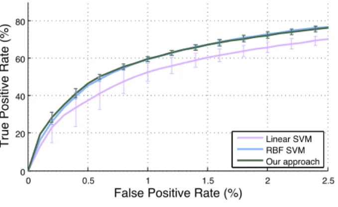
Fig. 4. Comparison of a linear SVM, RBF-SVM, and a linear SVM trained on the feature vectors described in Section VII-C and kernelized using the support vectors of an RBF-SVM. For classification of individual samples (ignoring structure), training a linear SVM on kernelized feature vectors yields a similar performance to a standard RBF-SVM. Error bars indicate standard deviation over 10 experiments on the hippocampus dataset with different samples randomly drawn from the training set.
andw0yi as their coefficients
w0yi= (αyi,1c(y
S
1, yi),· · ·, αyi,|S|c(y
S
|S|, yi))T, (19)
then the unary term can be re-expressed as
Di(yi) =hw0yi,gK,S(xi)i, (20)
which is of the finite-dimensional linear form needed for learning within the SSVM framework, as discussed in the previous section.
This suggests a simple 2-step learning approach to incor-porating kernels into an SSVM, illustrated in Fig. 3. First, we train a standard non-structured, non-linear kernel SVM to obtain a set of support vectors. These vectors are then used to create a set of kernel-transformed, or “kernelized”, feature vectors gK,S(xi), which are used to train the linear SSVM.
Although our formulation is not equivalent to a non-linear kernel SSVM2, nor does it intend to approximate a non-linear SSVM as kernel approximation methods do [39], [31], [56], it does produce models with the same functional form as those learned using a kernel SSVM. Most importantly, the resulting models perform well in practice as we will show later.
To demonstrate the principle that a linear SVM trained using kernel-transformed features performs similarly to a non-linear SVM that uses the same kernel, we conducted a simple proof-of-concept experiment for a classification task with a linear SVM classifying each sample independently while ignoring structure. We compare the performance of a standard linear SVM, an SVM trained with an RBF kernel, and a simplification of our approach in which kernelized feature vectors – obtained using the support vectors of the RBF-SVM – are used to train a standard linear SVM. The results in Fig. 4 support our intuition: So long as we transform the original feature vector using the right set of support vectors, learning the new coefficients under a different objective function (i.e., 2The parameters w0 now correspond to the primal variables of a linear SSVM instead of the dual variables of a non-linear SSVM.
as primal instead of dual variables) yields performance similar to a non-linear kernel SVM.
V. WORKINGSETS
We begin with a review of the stochastic subgradient method in the context of structured learning. We then introduce a novel technique to make the stochastic subgradient method more robust to approximation errors in the computation of subgra-dients using working sets of previously computed constraints.
A. The Stochastic Subgradient Method
The objective function of Eq. 6 can be minimized via a stochastic subgradient method [40], [32]. This class of meth-ods iteratively computes and steps in the opposite direction of a subgradient vector with respect to an example (Xn, Yn)
chosen by picking an index n ∈ {1. . . N} uniformly at random. This implies finding, at each step, the subgradient of the function
f(Yn, Y∗,w) =l(Yn, Y∗,w) +λ 2 ||w||
2
. (21)
A subgradient of the convex function f :W →R atw is
defined as a vectorg, such that
∀w0∈ W,gT(w0−w)≤f(w0)−f(w). (22)
The set of all subgradients at w is called the subdifferential
at w and is denoted ∂f(w). The subdifferential is always a
non-empty convex compact set.
For the hinge loss, a valid subgradient g(Yn, Y∗,w)with
respect to the parameterw can always be computed as: ∂f(Yn, Y∗,w)
∂w =ψ(Y
∗)−ψ(Yn) +λw. (23)
This results in a simple algorithm that iteratively computes and steps in the direction of the negative subgradient as described in Algorithm 1. In order to guarantee convergence, the step sizeη(t)needs to satisfy the following conditions:
lim T→+∞ T X t=1 η(t)=∞ and lim T→+∞ T X t=1 (η(t))2<∞. (24) Algorithm 1 SGD + inference 1: INPUTS :
2: D: Training set of N examples. 3: β : Learning rate parameter.
4: w(1) : Arbitrary initial values, e.g., 0. 5: OUTPUT :w(T+1)
6: fort= 1. . . T do
7: Pick some example (Xn, Yn)fromD
8: Y∗= arg max Y∈Yn(Sw(Y) + ∆(Y n, Y)) 9: η(t)← β t 10: g(t)← ∂f(Yn,Y,w(t)) ∂w(t) 11: w(t+1)←w(t)−η(t)g(t) 12: end for
For loopy CRFs, however, true subgradients of the hinge loss cannot always be obtained due to the intractability of loss-augmented inference, namely finding theY∗for each example.
This can lead to erratic behavior due to noisy subgradient estimates and loss of performance.
B. The Subgradient Method With Working Sets
Our algorithm aims at increasing the reliability of subgradi-ent methods by using working sets of constraints, denotedAn,
for learning loopy CRFs where exact inference is intractable. We first outline a batch version of our method in Algo-rithm 2 that uses subgradients computed as an average over the working sets of constraints. Later on, we will present a more efficient variant of this algorithm that uses atomic updates for every constraint in the working set. The batch version first solves the loss-augmented inference to find a constraint
Y∗ and add it to the working set An. It then steps in the
opposite direction of the approximate subgradient computed as an average over the set of violated constraints belonging to An.
Algorithm 2 Working sets + inference – batch version 1: INPUTS :
2: D: Training set ofN examples. 3: β : Learning rate parameter.
4: w(1) : Arbitrary initial values, e.g., 0.
5: OUTPUT :w(T+1)
6: InitializedAn← ∅for eachn= 1. . . N
7: fort= 1. . . T do
8: Pick some example(Xn, Yn)from D
9: Y∗= arg maxY∈Yn(Sw(Y) + ∆(Yn, Y))
10: An← An∪ {Y∗} 11: An0 ← {Y ∈ An | l(Y, Yn,w(t))>0} 12: η(t)← βt 13: g(t)← 1 |An0| P Y∈An0 ∂f(Yn,Y,w(t)) ∂w(t) 14: w(t+1)←w(t)−η(t)g(t) 15: end for
Hence unlike dual averaging methods [35], [58] that aggre-gate over all previous subgradients, our algorithm only con-siders the subset of active, namely violated, constraints when computing the parameter updates. Therefore all subgradients are computed with respect to the parameters at the current
iteration, as opposed to using their historical values. We will show that this produces better results in the experiments reported in Section VII.
We now analyze the convergence properties of the algorithm presented in Algorithm 2. Although finding true subgradients as defined in Eq. 22 cannot be guaranteed for loopy CRFs, interesting results can still be obtained even if one can only find an approximate-subgradientg, as defined in [47]:
∀w0:gT(w−w0)≥f(w)−f(w0)− (25)
The convergence properties of -subgradient methods were
studied in [41], [47], [40]. The “regret” or loss of the parameter vector w can be bounded by
Ekw(t+1)−w∗k22≤
G2 λ2t +
λ, (26)
whereGis a constant satisfying the condition||g||2≤G2and λ= C1. The re-derivation of this proof using our notations is
given in the appendix.
Given that the choice of the step size satisfies Eq. 24, we can see that the first term on the right side of Eq. 26 goes to 0 so stochastic-subgradient methods converge to a certain
distanceto the optimum. The key to improving convergence
is thus to obtain more accurate -subgradients, and we show
below how this could be achieved through the use of working sets.
Let g1, . . . ,gm ∈ Rd be the approximate subgradients of Lwith respect to example(Xn, Yn), for the labelings in the
working set An that still violates the margin constraint at a
given iteration. Assume that eachgi∈Rd comes from some distribution with meanµi∈∂L(w)and bounded variance.
Let δi = gi−µi be the difference between approximate
-subgradient gi and true -subgradient µi, and assume that
allδi are independent of one another. Note that, by definition,
each δi has zero expectation and hence their average δ¯ =
1
m
P
δi=m1 Pgi−m1 Pµi.
Therefore, using Hoeffding’s inequality [17] and the union bound, we can show that the average error δ¯ concentrates
around its expectation, i.e., 0 in this case, as the number of violated constraints in the working setm increases:
Pr δ¯ ≥r ≤2dexp −mr2 2G2 . (27)
The convexity of the subdifferential ∂L(w) implies that ¯
µ = m1 P
iµi ∈ ∂L(w). Therefore the probability of
g(t) , 1
m
Pg
i being more than a distance r away from any
true subgradient is bounded by Eq. 27 as well.
Algorithm 3 Working sets + sampling 1: INPUTS :
2: D: Training set of N examples. 3: Q : MCMC walker.
4: β : Learning rate parameter.
5: w(1) : Arbitrary initial values, e.g., 0.
6: OUTPUT :w(T+1)
7: InitializedAn← ∅for eachn= 1. . . N
8: fort= 1. . . T do
9: Pick some example (Xn, Yn)fromD
10: SampleY∗ according toQ(w(t), Yn) 11: An ← A ∪ {Y∗} 12: An0 ← {Y ∈ An |l(Y, Yn,w(t))>0} 13: z←w(t) 14: forY ∈ An0 do 15: g(t)← 1 |An0| ∂f(Yn,Y,z) ∂w(t) 16: η(t)← β t or η (t)←Line search(g(t)) 17: z←z−η(t)g(t) * atomic update * 18: end for 19: w(t+1)←z 20: end for
Given that the assumption of independence between all δi
might not always hold, we experimented with an adaptation of the batch version that replaces the standard update of Algorithm 2 with a sequence of atomic updates that has been shown to improve the rate of convergence [57]. We also introduce a second modification to Algorithm 2 where, instead
Algorithm 4 Working sets + inference 1: INPUTS :
2: D: Training set ofN examples. 3: w(1) : Arbitrary initial values, e.g., 0. 4: OUTPUT :w(T+1)
5: InitializedAn← ∅for eachn= 1. . . N
6: fort= 1. . . T do
7: Pick some example(Xn, Yn)from D
8: Y∗= arg maxY∈Y
n(Sw(Y) + ∆(Y n, Y)) 9: An← A ∪ {Y∗} 10: An0 ← {Y ∈ An | l(Y, Yn,w(t))>0} 11: z←w(t) 12: forY ∈ An0 do 13: g(t)← 1 |An0| ∂f(Yn,Y,z) ∂w(t) 14: η(t)← β t orη (t)←Line search(g(t)) 15: z←z−η(t)g(t) * atomic update * 16: end for 17: w(t+1)←z 18: end for
of stepping by an arbitrarily fixed distance in the subgradient direction, we choose the step size using a line search so as to best satisfy all currently active constraints, as explained in Section VI. The resulting method is outlined in Algorithm 4. In addition, the analysis presented in Section V-B suggests that it is possible to use a sampling method instead of the loss-augmented inference to obtain new constraints, and under similar assumptions the average subgradient ¯g still converges
to a valid subgradient. Based on this observation, we propose an adaptation of Algorithm 2 that uses sampling instead of solving the loss-augmented inference. This adaptation de-scribed in Algorithm 3 generates new constraints using an MCMC walker denotedQsimilar to the one described in [57].
VI. ADAPTIVESTEPSIZESELECTION
We aim at providing a systematic way to pick the step size by which to advance in the descent direction by minimizing a regularized loss. Instead of stepping by an arbitrarily fixed distance, we want to choose the step sizeη(t)that minimizes an objective function hAn,w(t)(η) that depends also on the current value of the parameters w(t) as well as the working
setAnthat contains all the constraints for examplengenerated
at the previous iterations, i.e.,
η(t)←arg min
η
hAn,w(t)(η). (28) More specifically, we would like to choose η(t) to ensure
that none of the previous constraints in the working set An
are highly violated at timet+ 1, namely after the subgradient
updatew(t+1)←w(t)−η(t)g(t). We thus define the function
hAn,w(t)(η)as hAn,w(t)(η) = max Y∈An l(Y n, Y,w(t+1) η ) + λ 2 w (t+1) η 2 = max Y∈An hD w(ηt+1), δψn(Y) E + ∆(Yn, Y)i + +λ 2 w (t+1) η 2 (29)
wherew(ηt+1)andδψn(Y)are shorthand notations:
w(ηt+1) = w(t)−ηg(t)
δψn(Y) = ψ(Y)−ψ(Yn), (30)
recalling that vectorψ(Y)is the feature map for labelingY.
The intuition is that hAn,w(t)(η) is a lower bound on the SSVM objective at w(ηt+1) with respect to example n, i.e.,
f(Yn, Y∗
w,w)(Eq. 21), and therefore an informative heuristic
for the line search in the negative subgradient direction. To simplify Eq. 29, we can remove the floor function[·]+ by adding an extra (trivial) constraint Yn to An since by
definitionl(Yn, Yn, ·)≡0andδψ n(Yn) =0. Hence hAn,w(t)(η) = max Y∈An + D w(ηt+1), δψn(Y) E + ∆(Yn, Y) +λ 2 w (t+1) η 2 , (31) whereAn +=An∪ {Yn}.
Since h is not the same quantity as the SSVM objective
function, minimizinghmay occasionally produce excessively
large step sizes, which impede convergence. To avoid this, we include a quadratic penalty on the magnitude by whichwcan
move in space, that is, w (t+1) η −w(t) = g(t) η. This
term is also known as a prox-function (i.e., proximity control function) which prevents overly large steps in the iterates and is commonly used in machine learning [21], [10]. This gives us the regularized line search objective function
hRAn,w(t)(η) =hAn,w(t)(η) +ρ(t) g (t) 2 η2, (32)
whereρ(t) is a regularization constant. We chooseρ(t)=Ct whereC is a constant value that can be determined by
cross-validation. Finally we choose the step sizeη(t)that minimizes
hR, i.e.,
η(t)←arg min
η
hRAn,w(t)(η). (33) To compute the minimum ofhR, we first observe that, by
expandingw(ηt+1) and after rearranging terms, Eq. 32 can be
explicitly written as hRAn,w(t)(η) = max Y∈An + λ 2 +ρ (t) g (t) 2 η2−Dg(t), δψn(Y) +λw(t) E η + λ 2 w (t) 2 +Dw(t), δψn(Y) E + ∆(Yn, Y) . (34)
It is easy to see that hR is the upper envelope of a set of
quadratic functions of η. In fact, since the quadratic term
does not depend on the specific constraint Y, the quadratic
upper envelope can be obtained easily by computing the cor-responding linear upper envelope, for which there are simple
O(mlogm)-time algorithms [18] where m is the number of
constraints being considered. The resulting envelope is then shifted vertically by the quadratic term, as shown in Figure 5. Let Y1, . . . , Ym ∈ An+ be the constraints that correspond to segments on the upper envelope andη1, . . . , ηm−1 be their intersections, both sorted left-to-right (visualized in Figure 5),
A
η f( η )B
η f( η )(a) Set of linear functions (b) Set of quadratic functions (c) Quadratic upper envelope
Fig. 5. Graphical illustration of the optimization problem posed by Eq. 34 for three random constraints shown in different colors. The two rows illustrate the two different cases explained in the main text:A) the minimum lies at the intersection itself,B) the minimum lies on the interior of one of the adjacent segments. In (a) and (b), the areas below the upper envelope are shaded in yellow. The solid lines in (a) represent the linear part ofhR, while those in (b) and (c) represent the full objective. Figure (c) shows the upper envelope over the three constraints with the optimalηshown in magenta.
given by the upper envelope. Let η0 = −∞ and ηm = ∞
for notational convenience, so that [ηi−1, ηi] is the interval
bounding the i-th segment of the upper envelope. The min-imum for each segment i can be computed in closed form
as the minimum of the parabola subject to the bounds of the interval, i.e., ηi∗= max ηi−1,min ηi, g(t), δψ n(Yi) +λw(t) λ+ 2ρ(t) g(t) 2 !! . (35) Let h∗(η∗i) denote its respective vertical values on the
parabola, which is equal to hR
An,w(t)(η
∗
i) since by definition
the segment of parabola ibetweenηi−1 andηi is part of the
upper envelope. Then η(t)is simply the η∗
i that results in the
smallest value of h∗, η(t)= arg min η∗ i∈{η ∗ 1,...,ηm∗} h∗(η∗i). (36)
In practice, we need only consider the two quadratic seg-ments on either side of the lowest intersection point, as shown in Fig. 5. The minimum must lie on either the intersection itself (case A) or the interior of one of the adjacent segments (case B), due to strong convexity and monotonicity of the upper envelope on either side of minimum. This helps to further reduce computational cost.
As outlined in Algorithm 4, the optimal step size η(t) for
each violated constraint inAn is computed using Eq. 33 – 36
and used to decide how far to move in the opposite direction of the corresponding approximate subgradient g(t). In order
to ensure convergence, we include a hard lower bound on the step-size in the algorithm to prevent it to converge to a point which is not optimal. In the supplementary material we show that the step sizeη(t)resulting for this procedure satisfies the conditions of convergence stated in Eq. 24.
VII. EXPERIMENTALRESULTS
In this section, we first introduce baselines against which we compare our approach. We then present our results on 2D and 3D data and discuss the length of the training times involved.
A. Multiple Versions of our Approach and Baselines
We will compare three versions of our approach
• Working sets + sampling. Compute each subgradient using the working set of constraints where instead of per-forming inference we use MCMC to sample constraints from a distribution targeting the loss-augmented score. We use a simple decreasing learning rate.
• Working sets + inference. Compute each subgradient using the working set of constraints where each constraint is computed by performing loss-augmented inference using graph-cuts or belief-propagation. We also use a simple decreasing learning rate.
• Working sets + inference + autostep. This is similar toWorking sets + inference but the decreasing learning rate is replaced by the adaptive step sizes of Section VI. against the following six baselines
• SVM.A linear SVM that classifies each sample indepen-dently without using a CRF.
• SSVM. The cutting plane algorithm introduced in [55] and discussed in Section II.
• SampleRank. The method proposed in [57] and also discussed in Section II.
• FW-Struct. The Frank-Wolfe algorithm for the L2-Loss SSVM [23]. We used the version without averaging known-as BCFW.
• SGD + inference. Loss-augmented inference using graph-cuts or belief-propagation. This is the subgradient descent (SGD) formulation of [40]. We try different values for the step sizeη(t)= β
t and use cross-validation
to determine the bestβin the interval[10−5, . . . ,10−10]. • SGD + sampling. Instead of performing inference, use MCMC to sample constraints from a distribution target-ing the loss-augmented score. This is equivalent to the method referred to as “SampleRank SVM” in [57]. In addition to these methods, we also experimented with aver-aging all past subgradients [35], [58], which did not produce competitive results for our biomedical tasks. We therefore did not include them in our comparison charts.
The loss-augmented inference of Eq. 7 required by the struc-tured methods was implemented using the maxflow library of [8] and the Loopy Belief Propagation implementation of [33].
In all cases, we used cross-validation on the training set to determine the regularization constants. All the methods were run for a sufficiently high number of iterations T = 1000
to ensure that they reach convergence. Because they involve randomization, the results for Working sets + samplingand
SampleRank were averaged over 5 runs.
The task loss ∆ of Eq. 5 is the per-superpixel weighted
loss ∆(Yn, Y) = P
i∈VI(yi 6= yin)r(yin). The term r(yni)
in the loss function weighs errors for a given class inversely proportional to the frequency at which it appears in the training data.
B. 2D Data
We performed segmentation of photon receptor cells in 2D retinal images. We use the publicly available UCSB retinal dataset,3which consists of 50 laser scanning confocal images of normal and 3-day detached feline retinas. The images were annotated by three different experts and the performance is measured by the Jaccard index commonly used for image segmentation [12]. The Jaccard index is the ratio of the areas of the intersection between what has been segmented and the ground truth, and of their union. It is written as
Jaccard index= True Positive
True Positive+False Positive+False Negative. The segmentation process begins by over-segmenting the images using SLIC superpixels [1]. For each superpixel, we extract a feature vector that captures texture information using
8×8 co-occurrence matrices and 10-bin intensity histograms. 3http://www.bioimage.ucsb.edu/research/biosegmentation
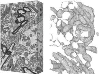
Fig. 7. Left. A second isotropic stack of neural tissue, similar to the one show in Fig. 1 but this time acquired from the striatum. This stack is made of318 872×1536 slices with around6-nanometer resolution in all three
directions.Right.3D rendering of the mitochondria found in a450×711×
318subvolume.
These feature vectors are used to train each baseline method, as well as our model. In a second set of experiments, we also transform the features using the kernel method described in Section IV. The original feature vectors are 74-dimensional and are thus mapped to a higher dimensional space. Example segmentations are shown in Fig. 6 and quantitative results are provided in Table I.
In the first line of this table, we compare our results against those of the six baselines using standard features. Working sets clearly improve performance over that of the baselines when using either Working sets + inference or
Working sets + sampling. Among the two, Working sets + inference yields the best results, at the cost of a higher-computational load as discussed in Section VII-D. Finally, also incorporating the adaptive step sizes, as in Working sets + inference + autostep, further improves performance. In the second line of the table, we use kernelized features instead of standard ones and observe exactly the same trends. We also see a performance increase due to the kernelized features by themselves.
C. 3D Data
Here we test our approach for the purpose of mitochondria segmentation from a 3D electron microscopy dataset. The segmentation of mitochondria and other organelles is a critical step for providing new insights into brain functionality, and has received a lot of interest from the computer vision and medical imaging communities [2], [20]. We use both the large and publicly available hippocampus stack4 depicted in Fig. 1 and a second stack from the striatum and depicted in Fig. 7.
We first over-segment the volume into supervoxels [1]. For each one, we extract a feature vector that captures local shape and texture information using Ray descriptors [30], intensity histograms and the following features computed at
SVM SSVM Sample- FW-Struct SGD + SGD + Working set Working set Autostep [55] Rank [57] [23] sampling inference [40] + sampling + inference
Original features 81.1% 89.4% 82.6% 89.4% 83.0% 87.2% 86.0% 89.8% 90.2%
Kernelized features 83.0% 90.1% 82.9% 90.3% 83.9% 87.6% 86.4% 91.4% 91.8%
TABLE I
SEGMENTATION PERFORMANCE FOR THE PHOTON RECEPTOR DATASET MEASURED IN TERMS OF THEJACCARD INDEX. THE LAST COLUMN REFERS TO THE METHODWorking sets + inference + autostep.
Ground truth SVM SGD + inference [40] Working set + inference
Fig. 6. Segmentation outlines obtained on one image of the photon receptor dataset using some of methods we tested overlaid in red.
Ground truth SVM SGD + inference [40] Working set + inference
Fig. 8. Outlines of mitochondria volumes obtained by different methods overlaid in red on a specific slice of the hippocampus dataset of Fig. 1. Our results are closer to the ground truth than the others.
SVM Lucchi SSVM Sample- FW-Struct SGD + SGD + Working set Working set Autostep [30] [55] Rank [57] [23] sampling inference [40] sampling inference
Original features 78.6% 80.0% 90.5% 82.6% 92.1% 85.4% 88.7% 87.1% 91.8% 92.9%
Kernelized features 82.3% - 92.7% 83.3% 92.7% 87.4% 89.2% 88.1% 94.4% 94.8% Hippocampus
SVM Lucchi SSVM Sample FW-Struct SGD + SGD + Working set Working set Autostep [30] [55] Rank [57] [23] sampling inference [40] sampling inference
Original features 81.5% 74.0% 90.0% 84.2% 88.8% 81.7% 84.8% 86.5% 90.1% 90.7%
Kernelized features 87.6% - 90.6% 89.6% 90.5% 87.9% 88.1% 90.2% 90.6% 92.1% Striatum
TABLE II
SEGMENTATION PERFORMANCE MEASURED IN TERMS OF THEJACCARD INDEX FOR THE TWOEMDATASETS. THE LAST COLUMN REFERS TO THE METHODWorking sets + inference + autostep.
five different scales: gradient magnitude, Laplacian of Gaus-sian and eigenvalues of the HesGaus-sian matrix, eigenvalues of the structure tensor. These feature vectors are used to train each baseline method, as well as our model. In a second set of experiments, we also transform the features using the kernel method described in Section IV. The original feature vectors are 140-dimensional and are thus mapped to a higher dimensional space. We trained a non-structured kernel SVM using the 140-dimensional standard features extracted from
N = 40000randomly sampled supervoxels. This yields a set
of 4223 support vectors for the striatum dataset and 4568 for the hippocampus that are then used to compute the transformed features.
In the case of the hippocampus dataset, due to the difficulty in obtaining labels for such large volumes, we performed our experiments on two subvolumes containing1024×768×165
voxels. The first subvolume was used to train the various methods while the second one was used for testing. Each subvolume contains∼13K supervoxels. The resulting graphs have∼91K edges. The same kind of splitting was also done
for the striatum dataset, which resulted in CRFs of similar sizes.
The mitochondria we find are depicted as 3D volumes in Figs. 1 and 7. Their outlines are overlaid in Fig. 8 on a single slice, along with those obtained using competing methods.
Performance is again measured by comparing 3D volumes against ground-truth ones in terms of the Jaccard index de-scribed in Section VII-B, but using volumes instead of areas. The corresponding results are provided in Table II. For [30], we use is a non-linear RBF-SVM classifier. The numbers exhibit the same trends as those discussed at the end of Section VII-B.
For the sake of completeness, we have also tested a very recent mitochondria segmentation method [45] that does not
rely on structured learning. Instead, it trains a cascade of classifiers at different scales and has been shown to outperform earlier algorithms based on Neural Networks, SVMs, and Random Forests on EM imagery. For the hippocampus and striatum datasets, it yields 83.8% and 83.5% Jaccard indices, which is much lower than what we obtain. The time required to train this method on our data (72605s) is also significantly longer than all those in Table III, and discussed in the next section.5
D. Training Cost
The time and memory required to train a classifier are important considerations for any Machine Learning approach. Concerning the memory requirements, the working set used by our approach does not lead to a significant increase in memory as we only need to store the feature maps, which are generally much more compact than the full labelings of the CRF.
While the linear SSVM is fast to train thanks to the use of kernelized features, the training of the first non-linear SVM used to transform the features can still potentially incur quadratic cost. Fortunately, it can be kept in check using known techniques such as randomly sampling the data or iteratively mining for hard examples [13]. However, these techniques cannot be used to directly speed up the SSVM though because they treat pixels as independent examples and disregard the structure of the graph.
We conducted a run-time analysis of the standard subgradi-ent method of [40] against the three versions of our algorithm discussed in this section. Table III gives the training time for each method for the same 1000 iterations, which is enough for all methods to have converged. Note, however, that Fig. 10 shows that Working sets + inference + autostep requires only about 200 iterations to converge. So, even though each iteration is a little slower due to the overhead attributable to maintaining the working set and doing a line-search,Working sets + inference + autostepyields in practice better solutions faster. Table III also shows that Working sets + samplingis much faster than solving the loss-augmented inference to find the most violated constraint.
5We used the publicly available Matlab implementation.
EM Photon receptor
SSVM [55] 43250s 1113s
SampleRank [57] 2524s 382s
SGD + Sampling 2481s 354s
Working sets + sampling 2619s (+5.5%) 370s (+4.5%)
SGD + inference [40] 5315s 438s
Working sets + inference 5842s (+9.9%) 492s (+12.3%)
Working sets + inference + autostep 6142s (+15.6%) 510s (+16.3%) TABLE III
TRAINING TIME REQUIRED TO REACH CONVERGENCE(T= 100
ITERATIONS FORSSVMANDT = 1000ITERATIONS FOR ALL OTHER METHODS)ON THEHIPPOCAMPUSEMDATASET. THE THREE VERSIONS OF OUR APPROACH DISCUSSED AT THE BEGINNING OFSECTIONVIIARE
LABELED IN BOLD. THE SLOWDOWN RESULTING FROM USING THE WORKING SET AND THE ADAPTIVE STEP SIZES IS SHOWN IN
PARENTHESES.
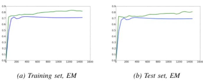
(a) Training set, EM (b) Test set, EM
Fig. 9. Learning curves showing the training and test scores (Jaccard index) on the Hippocampus dataset as a function of the number of iterationst. We report results for the sampling method with and without working set in green and blue respectively.
E. Generalization Error
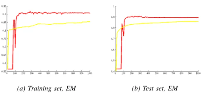
The evolution of the training scores and test scores as a function of the number of iterations is shown in Figs. 10 and 9. The parameters for the methods reported in these figures were found using cross-validation to avoid over-fitting. We have seen that all these methods could reach higher scores on the training set using different sets of parameters. Working sets + inference + autostep achieved the highest score on the training set and had to be regularized by increasing the value ofλ(increasingρ(t)also lead to a better generalization error). The curves in Fig. 9 clearly show that the working set of constraints produces much higher score on both the training and test sets. Fig. 10 shows thatWorking sets + inference + autostepsignificantly outperformsSGDon the training set as well as the test set. As shown in Table IV, it also outperforms
SSVMon the training set.
Hippocampus Striatum Photon receptor
SSVM 90.9% 86.3% 86.3%
Autostep 93.8% 90.6% 89.2% TABLE IV
TRAINING SCORES ACHIEVED BYSSVMANDWorking sets + inference + autostepUSING THE ORIGINAL FEATURES ON ALL THREE DATASETS.
(a) Training set, EM (b) Test set, EM
Fig. 10. Learning curves showing the training and test scores, expressed in terms of the Jaccard index, on the Striatum dataset as a function of the number of iterationst. We report results forWorking sets + inference + autostep
andSGD + inferencein red and yellow respectively.
F. Further Observations
1) Approximate subgradients: Our approach, and most of the existing methods presented in the related work section, all optimize the same objective function, given in Eq. 3, and rely on the computation of the most violated constraints. When these constraints cannot be obtained exactly, as is usually the case in image segmentation, the subgradient estimates are then necessarily only approximate. Certain methods, such as [55], require these quantities to be exact, while others, such as [40], [14] and [23], may work with approximate subgradients to obtain convergence up to a certain accuracy. The experi-mental results suggest that using a history of constraints as well as appropriate step sizes make learning more robust to approximation errors. An in-depth theoretical analysis of the accuracy of the subgradients will undoubtedly provide further insight into the behavior of this class of methods; though this is beyond the focus of this work, which is motivated by the need to improve performance in known applications.
2) Parameter selection for Kernelized features: While in certain cases kernel methods show improved performance compared with linear methods, they also introduce tuning parameters such as the number of support vectors. The kernel method presented in Section IV is not exempt from this difficulty. The selection of the number of support vectors for this method was done by cross-validation over the regulariza-tion constant λ and by empirically selecting an appropriate
number of training samples. The memory complexity of the linear SSVM is affected by the dimension of the kernelized features and is therefore another limiting factor that must be considered. We found empirically that the number of support vectors scale almost linearly with the number of training samples when fixing the regularization constantλ. In our case,
we found a training set of 40,000 samples to be a good trade-off between performance and training complexity.
3) Our Approach vsSSVM: Although SSVMtakes fewer iterations to converge, we found the cost per iteration to be much higher than SGD-based methods, which is mostly due to the higher cost of the loss-augmented inference. We hypothesize that the region of the space visited by SSVM
is highly non-submodular. One alternative to address this problem proposed in [50] is to perform the optimization over
a much smaller set of parameters for which exact optimization can be performed with graph-cuts.
4) Working sets + inferencevsWorking sets + inference + autostep: As stated earlier, all methods converged after at most 1000 iterations. The improvement due to the automatic step size selection reported in the experimental section is thus not due to a faster rate of convergence. Rather, we believe it to be attributable to the difficulty of manually setting the right step size at each iteration. We found empirically that different step size selections can occasionally yield improvements on specific datasets but we did not find a specific one that would perform well for all datasets. We thus opted for the standard decreasing schemeη(t)=β
t that gave the best results overall.
VIII. CONCLUSION
Understanding neural connectivity, function, and structure of the brain requires detailed 3D models. Although new imaging techniques such as FIB-SEM allow neuroscientists to visualize the brain in great detail, these crucial models are mostly still traced by hand. To eliminate this barrier to progress, new automatic segmentation techniques for identify-ing structures of interest in these rich datasets are required.
To address this need, we have presented a new segmentation framework that nearly achieves a human level of performance, raising the bar over previous methods, including our own earlier work. To this end, we introduced three key innovations, including a technique to leverage the power of non-linear kernels in a structured prediction framework as well as a working set based approximate subgradient method with line-search to learn graphical models when inference is challeng-ing. Our method is particularly appealing for learning large CRFs with loops, which are common in computer vision tasks, since under these circumstances the use of working sets of constraints makes the subgradient method more robust to approximation errors and produce higher-quality solutions.
The benefits of our approach were clearly demonstrated on 2D confocal optical images and 3D EM image stacks, but it is important to note that our method is general and can be applied to imagery from any type of microscopy.
REFERENCES
[1] R. Achanta, A. Shaji, K. Smith, A. Lucchi, P. Fua, and S. Susstrunk. SLIC superpixels compared to state-of-the-art superpixel methods.
IEEE Transactions on Pattern Analysis and Machine Intelligence,
34(11):2274–2282, Nov 2012.
[2] B. Andres, U. Koethe, M. Helmstaedter, W. Denk, and F. Hamprecht. Segmentation of SBFSEM Volume Data of Neural Tissue by Hierarchi-cal Classification. InDAGM Symposium on Pattern Recognition, volume 5096 ofLecture Notes in Computer Science, pages 142–152, 2008. [3] M.-F. Balcan, A. Blum, and S. Vempala. Kernels as features: On kernels,
margins, and low-dimensional mappings. Machine Learning, 65(1):79– 94, Oct 2006.
[4] L. Bertelli, T. Yu, D. Vu, and B. Gokturk. Kernelized Structural SVM Learning for Supervised Object Segmentation. InConference on
Computer Vision and Pattern Recognition, pages 2153–2160, 2011.
[5] D. Bertsekas.Nonlinear Programming. Athena Scientific, 1999. [6] J. Besag. Spatial Interaction and the Statistical Analysis of Lattice
Systems. J. Roy. Statist. Soc. B, 36(2):192–225, 1974.
[7] Y. Boykov and M. Jolly. Interactive Graph Cuts for Optimal Boundary & Region Segmentation of Objects in N-D Images. InInternational