© 2011 IEEE. Reprinted, with permission, from Madhu Goyal, Feature Selection of Imbalanced Gene Expression
Microarray Data . Software Engineering, Artificial Intelligence, Networking and Parallel/Distributed Computing
(SNPD), 2011 12th ACIS International Conference on, July 2011. This material is posted here with permission of the
IEEE. Such permission of the IEEE does not in any way imply IEEE endorsement of any of the University of
Technology, Sydney's products or services. Internal or personal use of this material is permitted. However, permission
to reprint/republish this material for advertising or promotional purposes or for creating new collective works for
resale or redistribution must be obtained from the IEEE by writing to [email protected]. By choosing to
view this document, you agree to all provisions of the copyright laws protecting it
Feature Selection of Imbalanced Gene Expression Microarray Data
Ali Anaissi
(Author)
Center of Quantum Computation and Intelligent Systems (QCIS), Faculty of Engineering and
Information Technology (FEIT), University of Technology, Sydney (UTS)
Broadway NSW 2007, Australia
E-mail: [email protected]
Madhu Goyal
(Author)
Center of Quantum Computation and Intelligent Systems (QCIS), Faculty of Engineering and
Information Technology (FEIT), University of Technology, Sydney (UTS)
Broadway NSW 2007, Australia
E-mail: [email protected]
Paul J. Kennedy
(Author)
Center of Quantum Computation and Intelligent Systems (QCIS), Faculty of Engineering and
Information Technology (FEIT), University of Technology, Sydney (UTS)
Broadway NSW 2007, Australia
E-mail: [email protected]
Abstract— Gene expression data is a very complex data set characterised by abundant numbers of features but with a low number of observations. However, only a small number of these features are relevant to an outcome of interest. With this kind of data set, feature selection becomes a real prerequisite. This paper proposes a methodology for feature selection for an imbalanced leukaemia gene expression data based on random forest algorithm. It presents the importance of feature selection in terms of reducing the number of features, enhancing the quality of machine learning and providing better understanding for biologists in diagnosis and prediction. Algorithms are presented to show the methodology and strategy for feature selection taking care to avoid overfitting. Moreover, experiments are done using imbalanced Leukaemia gene expression data and special measurement is used to evaluate the quality of feature selection and performance of classification.
Keywords- feature selection; random forest; imbalanced data; cost sensitive learning.
I. INTRODUCTION
Many features are available in gene expression microarray data with a small number of observations. It implied that many genes are redundant and irrelevant to a specific outcome of interest. Consequently, a small set of these genes are related to the desired output and can be used in prediction and classification. As this data has a small size number of samples and their dimensionality is very large with correlated variables, feature selection becomes a big challenge and represents a real prerequisite in the field of bioinformatics [1] [2] [3] [4].
Feature selection is a technology used to select a subset of genes that represents the most important and relevant features by removing the redundant and irrelevant features from a given data set. Many potential benefits can be achieved in feature selection. The first one is reducing a high dimensional data set into lower dimension by removing the noise and irrelevant information. Reducing the effect of the curse of dimensionality and enhancing the quality of dimensionality reduction algorithm especially the non-linear ones which mostly based on distance measurement. The third advantage is increasing the speed of learning algorithm such as classification, similarity measurement and prediction. The last one is providing better understanding for biologists and assists them in diagnosis and prediction.
This work is motivated by a childhood gene expression data set for Leukaemia malignancy. The data set is very complex and it consists of a small number of patients with a very large number of correlated features. Patients are imbalanced separated based on the risk type of the malignancy. Biologists want to know which subset of features plays the main role in discrimination between these patients based on the risk type. According to the characteristics of the given data set, a feature selection technique is presented for this issue with ability to handle the dependencies between features and imbalanced data.
The rest of this paper is organized as follows. Section II introduces the different techniques of feature selection. Section III explains the random forest and how it is very suitable for gene expression data. We will discuss the evaluation measures for feature selection based on the classifier performance in Section IV. Section V discusses the different methods to deal with imbalanced data. Section
VI presents the methods and algorithms used in this work to attain the desired quality of features selection. Section VII discuses the obtained results and calculate the accuracy and precision of classification performance. In Section VIII, we draw conclusions about the results and present some of the future work.
II. FEATURE SELECTION TECHNIQUES
There are three general approaches for feature selection. The first one is concerning feature selection regardless of the classifier. This method is known as filtering technique. It aims to calculate the importance of each feature and then select the top rank. This method is simple, fast and easily scales to very high dimensional data. However, it has some drawback as most of the proposed filter techniques are univariate (t-test and ANOVA [5]). This means that each feature is considered and treated separately, thereby ignoring the correlation between features. On the other hand, gene expression data set is considered as highly correlated features. As a result, a worse misclassification performance arises comparing to other feature selection techniques.
The second approach participates in prediction and how to build a good classifier. This method is known as a wrapper selection (e.g. Genetic algorithms [6]) which aims to select a subset of features that are useful to build a good classifier or predictor. The advantage of this technique is the ability to take into account the correlation between features and the interaction with the classifier. However, this technique has some drawbacks as it prones to a high risk of over fitting and it is very intensive computation.
The last approach is the embedded method (ex: Random forest [7]). It is similar to wrapper technique with less computation and less risk of over fitting. In this paper, we will use the embedded technique to select the most relevant subset feature that will have a good performance in classification and prediction. Moreover, Random forest will be interpolated in this technique to measure the importance of the features and evaluate the classification performance.
III. RANDOM FOREST ALGORITHM
Random forest is an ensemble classifier that consists of many decision trees. Many classification trees are grown in order to classify an input sample. These trees start voting for each class type. The class with higher number of votes win the classification.
During the construction of each tree, about one-third of the cases are left out of the sample. This out-of-bag data is used to estimate the classification error. In addition to the out-of-bag estimations, random forest generates the importance measurements of each input features based on the out-of-bag error and class votes. Based on these measurements, features are selected with a high importance value.
As feature elimination decision should be taken precisely, Random Forest is very suitable for microarray data. It uses
ensemble classifiers for feature selection instead of use one particular classifier and accepts its outcome as a final result. In other words, features will not be deleted based on one decision or one tree, but many trees will decide and confirm this decision of elimination. Another characteristic of Random Forest is that it is applicable on a very high dimensional data with a low number of observations and high correlated variables. These two characteristics represent the main description of microarray data sets. The last common characteristic between Random Forest and Microarray is that random forest can handle missing data and unbalanced classes. In microarray data, it is rare to have balanced classes and without any missing features. For example, in the target data set, the patients are classified into three categories (high, medium, and standard risk) and the medium risk category has the majority in the data set.
Random forest consists of several steps 1. Choose T—number of trees to grow.
2. Choose m—number of variables used to split each node. m << M, where M is the number of input variables. m is hold constant while growing the forest.
3. Grow T trees. When growing each tree do the following. (a) Construct a bootstrap sample of size n sampled from Sn with replacement and grow a tree from this
bootstrap sample.
(b) When growing a tree at each node select m variables at random and use them to find the best split.
(c) Grow the tree to a maximal extent.
4. To classify point X collect votes from every tree in the forest and then use majority voting to decide on the class label.
Finally, the algorithm produces a ranked list of feature’s importance with a classification error rate. The top features, which represent the most significant and relevant features, will be selected based on the importance measurements. Then the above four steps are repeated until the error rate reach the minimum value and before going back in increasing.
As imbalanced problem should be considered while applying random forest, a performance measurement is another factor that should be also considered to evaluate the classification of imbalanced data.
IV. EVALUATION MEASURES OF IMBALANCED DATA As our target data is extremely imbalanced, the minor class has a very little impact on the accuracy measurement. This yields to a fact that the traditional accuracy measure cannot be an adequate performance measure in a case of extremely imbalanced data. Other measures have been proposed for imbalanced data evaluation of the classification performance measure. Most of these measurements rules are based on the data obtained from the confusion matrix. Confusion matrix represents the outcome of the actual predicted classification obtained by the classifier. Table 1 illustrates a confusion matrix for a two-class two-classification. Conventionally, the majority two-class is
represented as a negative class label and the minority class is represented is as a positive class label. The actual class label of the examples presented in the first column, and their predicted class label presented in the first row. The numbers of positive and negative examples that are classified correctly are denoted by TP and TN, while the misclassified examples are denoted by FN and FP.
Table 1. A confusion matrix for a two-class classification
Predicted positive class Predicted negative class Actual positive class
Actual negative class
True Positive(TP) False Negative(FN) False Positive(FP) True Negative(TN)
In order to measure the performance of the classifier, the accuracy should be determined for each class separately; i.e. the true negative rate and the true positive rate which shown in equation 1 and 2, respectively. These two estimated values also known as Recall.
Recall+=True Negative Rate=
FP
TN
TN
+
(1) Recall-=True Positive Rate=FN
TP
TP
+
(2) Another interested measure is the precision of thepredictive positive and negative cases which is the proportion of the correct predicted positive cases and negative cases, respectively. This can be determined using equation 3 and 4. Precision+=
FP
TP
TP
+
(3) Precision-=FN
TN
TN
+
(4) These presented measures will be adopted to evaluate the performance of the classifier after applying feature selection and removing the redundant and irrelevant features.V. METHOD TO SOLVE THE IMBALANCED PROBLEM Our target gene expression data set has a problem of imbalance; i.e., classes or patients are not balanced distributed and some patients represent a very small minority class. An example of this problem is that patients with high risk have a minority number in the data set comparing to the patients with medium risk. Features of the majority classes dominate the learning algorithm and make features in the minority classes difficult to be fully recognized. This yields to unsatisfactory classification performance.
Two different approaches have been proposed to overcome this problem. The first approach is known as sampling technique. This solution aims to alter the distribution of the classes toward more balanced classes. This can be done either by over sampling technique or down sampling technique and sometimes both [11].
Down sampling is a technique used to remove a number of observations in such way from the majority class. It aims to attain the sample number of the majority class as in the minority class. SHRINC, which is an algorithm proposed by Kubat et al. (1997) [10], is used for down sampling technique by reducing the number of sample of the majority class.
This method has some drawbacks because it can eliminate some useful information. Moreover, as we showed in the above discussion about the gene expression data set, a very small number of observations are available in the target gene expression data. Consequently, elimination of observations is not allowed for the target data set.
On the other hand, over sampling technique aims to increase the minority class by replicating the minority sample so that they reach the same size as the majority class. The synthetic minority over sampling technique (SMOTE) [11] is an approach used to form new minority class examples by interpolating between several minority classes examples that lie together. The main key of this method is based on the k-nearest neighbours and it is based on the distance measure, thus; it cannot work on a very high dimensional data set like our data set due to the curse of dimensionality.
The second approach to tackle the problem of imbalanced data is the cost sensitive learning [8] [9] [12]. This can be achieved by assigning a high cost to misclassification of the minority class and vice versa. Based on the above discussion about sampling technique, this method is more suitable on the target data and for learning extremely imbalanced data. One question is asked; how cost sensitive learning can be used with random forest. Random forest produces votes from each generated tree in the forest. These votes then used to classify a point or observation. The majority voting decides the class label of the input point. Cost sensitive learning will be applied on these votes by assigning weight for each class. A higher misclassification error cost is given to the minority class by assigning a larger weight. These weights will play a role in calculating the votes at the terminal nodes. The weighted vote of a class is the weight for that class times the number of cases for that class.
As random forest builds each tree from a bootstrap sample, another approach has been proposed to help and support cost sensitive learning. This approach aims to induce random forest to constitute tree from a balanced bootstrap sample. i.e., a bootstrap sample is drawn from the minority class with the same number of cases from the majority class.
VI. STRATEGY APPLIED FOR FEATURE SELECTION In this paper we propose a strategy composed of different methods and algorithms to address the problem of imbalanced data and select the most relevant features. These algorithms are presented in several steps which are shown in the following paragraphs.
A. Step 1. Algorithm to Find the Best Training Error Cost for Each Class.
Based on the discussion about the imbalanced data and as we proposed to use the cost sensitive learning to handle this problem, The first step was to find the best weight to assign for each class. Knowing that, each tree is built by taking samples from each class with the size number same as the number of the minor class i.e.; balanced samples. An algorithm has been developed to find these weights and it is presented in the next paragraph.
Let D is the number of features and N is number of patients.
1. Select m features random sample from the data set where m <<D
2. Loop1:
2.1 Assign randomly an error cost for each class 2.2 Loop2:
2.1.1 Run random forest on this sample with the assigned error cost
2.1.2 Read the out-of-bag error(oob) and the importance values for each feature
2.1.3 Delete features with importance <=0 2.1.4 If oob<previous oob
Then continue Loop2 on the selected features
2.1.5 Else if oob is relatively acceptable as well as the precision, then save assigned error cost values and exit.
2.1.6 Else continue Loop1 and assigned a new cost error values
After running this algorithm and determining the error cost values, these values are examined on other random samples to ensure that they are well selected and can make the data more balanced for different samples. The reason for selecting a random sample in the above algorithm is that the data set is a very complex data and has very large number of the features. As a result, the above algorithm will be impractical if it is run on the full data set.
B. Step 2. Algorithm to Select the Important Features.
After determining the error cost values for each class, the next step is to start running random forest and select the most important and relevant features based on the desired class label i.e. risk type. As we said before, it is impractical to run the random forest on the full data set. A strategy has been followed for this issue. The data is randomly divided into different samples. Then we run random forest on each sample and accumulate the result in a one data set.
After that, the accumulated data set is used and random forest start running in several iterations. In each iteration, features with small importance value are removed until the out-of-bag error and number of selected features becomes stable or the out-of-bag error goes up. The next paragraph presents the algorithm of this method.
1. Divide the data randomly into different samples (without replacing)
2. For n=1: number of samples
2.1 Run random forest sample number n
2.2 Read the out-of-bag(oob) and the importance values for each feature
2.3 Delete features with importance <=0
2.4 Accumulate the selected data in Predefined matrix M
End 3. Do
3.1 Run random forest on the matrix M
3.2 Read the out-of-bag(oob) and the importance values for each feature
3.3 Delete features with importance <=0
While oob<previous oob and the precision of each class is acceptable (Another criteria to stop running random forest is when the selected features become stable).
C. Step 3. Algorithm to Avoid Overfitting in Feature Selection
Although random forest uses the cross-validation technique and it produces the out-of-bag error which is similar to out of sample test. Another strategy has been followed to ensure that the selected features are useful and has a good performance in classification. Furthermore, this strategy also aims to ensure that the algorithm will not overfit or overtraining. Consequently, the data is decomposed into two data sets; train and test data. Based on algorithm 2, the train data is processed in the first loop. After ending this loop, the test data is read and irrelevant features are eliminated based on the features selected from the train data in the first loop and test data is attached to the train data. This mean that we have a completely train data and a heterogeneous data that contains test and train data. The second loop is continued on the train data as in the algorithm 2 but in each iteration, the heterogeneous data is filtered by eliminating features based on the random forest of the train data and then evaluate the classification of the filtered test data and read the out-of-bag error. At the instance that the out-bag-error is going back in increasing on the heterogeneous data, processing should be ended because it is the beginning of the over-training. The next paragraph illustrates this algorithm.
1. Divide the data into two data sets train and test.
2. Divide the train data randomly into different samples (without replacing)
3. For n=1: number of samples
3.2 Read the out-of-bag-train error(oob) and the importance values for each feature
3.3 Delete features with importance <=0
3.4 Accumulate the selected data in Predefined matrix M
End
4. Filtered the test data by keeping the features selected from the train data and bind them to the train data 5. Do
5.1 Run random forest on the matrix M(train) 5.2 Read the out-of-bag-train error and the
importance values for each feature
5.3 Delete features from the train data with importance <=0 as well as the test data
5.4 Run random forest on the filtered test data and read the out-of-bag-test error of test data
While out-of-bag-test <previous out-of-bag-test (Another criteria to stop running random forest is when the selected features become stable).
VII. DATA SET
Gene expression data is very complex data set that characterized by its high dimensionality with a low number of observations. Another characteristic of gene expression data is the correlation between features. A feature that is completely useless by itself can provide a significant performance improvement when taken with others. Another difficulty can be faced in gene expression data is the imbalanced data; i.e., at least one of the classes has very small samples and considered as a minor sample.
A gene expression data set has been used in this study for validation and experiments. It is collected from Westmead hospital for children. The data is about childhood Leukaemia and it is composed of 110 patients with 22,278 features. The patients are classified into 3 classes
Medium risk (78 patients) Standard risk (21 patients) High risk (11 patients)
As can be seen from the distribution of the classes, the data is extremely imbalanced where the patients with medium risk is overcome the data set and makes the classifier tends to be biased towards this majority class. Moreover, the data set has a very small number of observations or patients comparing to the number of features which also pose feature selection to a great challenge and complex computation.
VIII. EXPERIMENTS AND RESULTS
As the first step was to solve the imbalanced problem, the first algorithm is executed and training error cost are determined for each class. These weights are:
High: 0.05973619
Medium: 0.06548166
Standard: 0.06247892
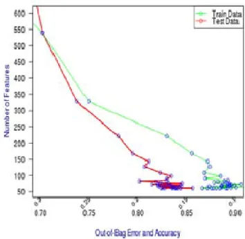
Using these weights and with the helping of the balance sample size of each tree, relevant features have been selected with good performance classification for each class and specially the minor class. Ninety five features out of the 22,278 have selected during this processing with a good performance classification. Ninety eight patients have been used for training and 12 patients for testing. Figure 1 presents graphically the processing of the algorithm by plotting the out-of-bag error for the test and train data in contrast to the number of features. As can be seen from the graph and based on the train data, the out-of-bag error is in decreasing as the number of irrelevant features and noise are eliminated in each iteration. After several iterations, the out-bag-error become stable in a range between 0.07 and 0.04 with the number of features also stable around the number 95 and 61. With respect to the test data, the classification performance is quite similar to the train data with less accuracy.
Figure 1: Out-of -bag error during processing
Moreover, it can be noticed during the processing that there is no over training of the data where the out-of-bag error of the test data is not increasing after several iteration. Confusion matrix shown in table 2 resulted after completion the execution of the training algorithm. As can be seen from this matrix, patients with high risk are full predicted. Sixty nine patients with standard risk are predicted correctly. However, two patients are predicted as high risk and one patient as standard risk. With respect to the standard risk patients, sixteen patients are predicted correctly and only one patient is predicted as a medium risk.
Based on the performance measurement which discussed before, several calculations are done to show the accuracy and precision of the classifier after features selection. The precisions of the high, medium and standard class are 81.8 %, 98.5% and 94.1% respectively. However, the accuracy of the high, medium and standard are 100%, 95.8% and 94.1% respectively (Table 3).
Table 1: Confusion matrix of the training data
High Medium Standard
High 9 0 0
Medium 2 69 1
Standard 0 1 16
Table 2: Precision and accuracy of classification
Precision Accuracy
High risk 0.818 1 Medium risk 0.985 0.958 Standard risk 0.941 0.941
IX. CONCLUSION AND FURTHER STUDY
In this paper we have proposed a methodology to select the relevant and important features of an imbalanced gene expression data set. The data was about leukaemia childhood malignancy and features are selected based on the risk type of the patients. Random forest has been used in this methodology with the consideration of the imbalanced data. We have discussed the important of features selection in the field of bioinformatics and how it is shifted to become essential step before applying any machine learning algorithms. We also presented the different techniques of feature selection and we shown how the embedded method and random forest is one of the most suitable techniques for feature selection of imbalanced gene expression data. Moreover, we have shown in this paper different methodology to solve the imbalanced problem and how ‘cost sensitive learning’ technique is might be the only method can be applied on the imbalanced gene expression data.
Different rules are also presented in this paper to measure the classification performance of imbalance data. Then we presented the experiments done for this work and we shown the outcome of the classification after selecting the most important and relevant features which summarized in the confusion matrix.
Based on the obtained result from the Leukaemia gene expression data set, there is no doubt that the outcome was very acceptable where almost all the patients are correctly predictive with a small subset of features rather than the 22,678.
With respect to the imbalanced problem, it can be implied that the cost-sensitive learning performed a good mission in making the High risk patients are fully recognized and classified. On the other hand, neither over-sampling nor down-sampling technique cannot be applied on these kinds of data sets. We can also imply from these experiments that the cost-sensitive learning is doing well on the large datasets.
Another factor that deserves to be considered in these studies is the over-fitting problem. We have shown in this paper how the over-fitting problem can be avoided by evaluating the classification performance and checking the out-bag error for the test data set along with processing of the train data. However, in this experiment we have not reached the overtraining level.
REFERENCES
[1] Varshavsky R, et al. Novel unsupervised feature filtering of biological data. Bioinformatics 2006; 22:e507-e513.
[2] Guyon I, Elisseeff A. An introduction to variable and feature selection. J. Mach Learn Res. 2003; 3:1157-1182.
[3] Alon U, et al. Broad patterns of gene expression revealed by clustering analysis of tumor and normal colon tissues probed by oligonucleotide arrays. Proc. Nat. Acad. Sci. USA 1999; 96:6745-6750.
[4] Ben-Dor A, et al. Tissue classification with gene expression profiles. J. Comput. Biol. 2000; 7:559-584.
[5] Jafari P, Azuaje F. An assessment of recently published gene expression data analyses: reporting experimental design and statistical factors. BMC Med. Inform. Decis. Mak. 2006; 6:27.
[6] Li L, et al. Gene selection for sample classification based on gene expression data: study of sensitivity to choice of parameters of the GA/KNN method. Bioinformatics 2001; 17:1131-1142
[7] Breiman, L., 2001. Random Forests. Machine Learn. 45, 5–32. [8] Domingos, P. (1999). Metacost: A general method for making
classifiers cost-sensitive. In Proceedings of the 5th ACM SIGKDD International Conference on Knowledge Discovery and Data Mining, (pp. 155–164)., San Diego. ACM Press.
[9] Pazzani, M., Merz, C., Murphy, P., Ali, K., Hume, T., & Brunk, C. (1994). Reducing misclassificationcosts. In Proceedings of the 11th International Conference on Machine Learning, San Francisco. Morgan Kaufmann.
[10] Kubat, M., Holte, R., & Matwin, S. (1998). Machine learning for the detection of oil spills in satellite radar images. Machine Learning, 30, 195–215.
[11] Chawla, N. V., Lazarevic, A., Hall, L. O., & Bowyer, K. W. (2003). SMOTEboost: Improving predictionof the minority class in boosting. In 7th European Conference on Principles and Practice of Knowledge Discovery in Databases, (pp. 107–119).
[12] Charles Elkan, “The Foundations of Cost-Sensitive Learning,’’ the Seventeenth International Joint Conference on Arti_cial Intelligence, pp. 973-978