Targeted Minimum Loss Based Estimation of an Intervention Specific Mean Outcome

University of California, Berkeley

U.C. Berkeley Division of Biostatistics Working Paper Series

Year  Paper

Targeted Minimum Loss Based Estimation of

an Intervention Specific Mean Outcome

Mark J. van der Laan

Susan Gruber

∗_{Division of Biostatistics, School of Public Health, University of California, Berkeley,}

[email protected]

†_{Division of Biostatistics, School of Public Health, University of California, Berkeley,}

[email protected]

This working paper is hosted by The Berkeley Electronic Press (bepress) and may not be commer-cially reproduced without the permission of the copyright holder.

http://biostats.bepress.com/ucbbiostat/paper290 Copyright c2011 by the authors.

Targeted Minimum Loss Based Estimation of

an Intervention Specific Mean Outcome

Mark J. van der Laan and Susan Gruber

Abstract

Targeted minimum loss based estimation (TMLE) provides a template for the construction of semiparametric locally efficient double robust substitution esti-mators of the target parameter of the data generating distribution in a semipara-metric censored data or causal inference model based on a sample of independent and identically distributed copies from this data generating distribution (van der Laan and Rubin (2006), van der Laan (2008), van der Laan and Rose (2011)). TMLE requires 1) writing the target parameter as a particular mapping from a typ-ically infinite dimensional parameter of the probability distribution of the unit data structure into the parameter space, 2) computing the canonical gradient/efficient influence curve of the pathwise derivative of the target parameter mapping, 3) specifying a loss function for this parameter that is possibly indexed by unknown “nuisance” parameters, 4) a least favorable parametric submodel/path through an initial/current estimator of the parameter chosen so that the linear span of the gen-eralized loss-based score at zero fluctuation includes the efficient influence curve, and 5) an updating algorithm involving the iterative minimization of the loss-specific empirical risk over the fluctuation parameters of the least favorable para-metric submodel/path. By the generalized loss-based score condition 4) on the submodel and loss function, it follows that the resulting estimator of the infinite dimensional parameter solves the efficient influence curve (i.e., efficient score) equation, providing the basis for the double robustness and asymptotic efficiency of the corresponding substitution estimator of the target parameter obtained by plugging in the updated estimator of the infinite dimensional parameter in the tar-get parameter mapping.

To enhance the finite sample performance of the TMLE of the target parame-ter, it is of interest to choose the parameter and the nuisance parameter of the

loss function as low dimensional as possible. Inspired by this goal, we present a particular closed form TMLE of an intervention specific mean outcome based on general longitudinal data structures. %We also present its generalization of this type of TMLE to other causal parameters. This TMLE provides an alternative to the closed form TMLE presented in van der Laan and Gruber (2010) and Stitelman and vanderLaan (2011) based on the log-likelihood loss function. The theoretical properties of the TMLE are also practically demonstrated with a small scale sim-ulation study. The proposed TMLE builds upon a previously proposed estimator by Bang and Robins (2005) by integrating some of its key and innovative ideas into the TMLE framework.

1

Introduction.

Many studies generate data sets that can be represented asnindependent and identically distributed observations on a specified longitudinal data structure. By specifying a causal graph (Pearl (1995), Pearl (2000)), or equivalently, a system of structural equations specifying the observed variables as a function of a set of observed parent variables and an unmeasured exogenous error term, one codes the assumptions needed to be able to define a post-intervention distribution of this longitudinal structure that represents the distribution the data would have had under a specified intervention on a subset of the nodes defining the observed longitudinal data structure. Causal effects are defined as parameters of a collection of post intervention distributions.

A current and important topic is the estimation of causal effects of setting the value of multiple time point intervention-nodes on some final outcome of interest based on observing n independent and identically distributed copies of a longitudinal data structure. In particular, one might be concerned with estimation of the mean of the outcome under the post-intervention distribu-tion for a specified multiple time point intervendistribu-tion. Under a causal graph and a so called sequential randomization and positivity assumption, one can identify the latter by the so called G-computation formula which maps the distribution of the observed longitudinal data structure on the experimental unit into the post-intervention distribution of the outcome. In this article we consider estimation of this intervention specific mean outcome in a semipara-metric model that only makes statistical assumptions about the intervention mechanism, where the latter is defined by the conditional distribution of the intervention node, given the parent nodes of the intervention node, across the intervention nodes.

Different type of estimators of the intervention specific mean outcome in such a semiparametric model have been proposed. These estimators can be categorized as inverse probability of treatment/censoring weighted (IPTW) es-timators, estimating equation based estimators based on solving an estimating equation such as the augmented IPTW estimating equation, maximum like-lihood based G-computation estimators based on parametric models or data adaptive loss-based learning algorithms, and targeted maximum likelihood (or more general, minimum loss-based) estimators defined in terms of an initial estimator, loss function and least favorable fluctuation submodel through an initial or current estimator that is used to iteratively update the initial es-timator till convergence. The IPTW eses-timator relies on an eses-timator of the intervention mechanism, the maximum likelihood estimator relies on an es-timator of the relevant factor of the likelihood, while the augmented IPTW

estimator and TMLE utilize both estimators. The augmented IPTW and the TMLE are so called double robust, and locally asymptotically efficient. The TMLE is also a substitution estimator and is therefore guaranteed to respect the global constraints of the statistical model and target parameter mapping. IPTW estimation is presented and discussed in detail in (Robins, 1999; Hernan et al., 2000). Augmented IPTW is originally developed in Robins and Rotnitzky (1992). Further development on estimating equation method-ology and double robustness is presented in (Robins et al., 2000; Robins, 2000; Robins and Rotnitzky, 2001) and van der Laan and Robins (2003). For a detailed bibliography on locally efficient estimating equation methodology we refer to Chap. 1 in van der Laan and Robins (2003).

For the original paper on TMLE we refer to van der Laan and Rubin (2006). Subsequent papers on TMLE in observational and experimental studies include Bembom and van der Laan (2007), van der Laan (2008), Rose and van der Laan (2008, 2009, 2011), Moore and van der Laan (2009a,b,c), Bembom et al. (2009), Polley and van der Laan (2009), Rosenblum et al. (2009), van der Laan and Gruber (2010), Stitelman and van der Laan (2010), Gruber and van der Laan (2010b), Rosenblum and van der Laan (2010), Wang et al. (2010), and Stitelman and van der Laan (2011b). For a general comprehensive book on this topic, which includes most of these applications on TMLE and many more, we refer to van der Laan and Rose (2011). An original example of a particular type of TMLE (based on a double robust parametric regression model) for estimation of a causal effect of a point-treatment intervention was presented in Scharfstein et al. (1999) and we refer to Rosenblum and van der Laan (2010) for a detailed review of this earlier literature and its relation to TMLE. van der Laan (2010) and Stitelman and van der Laan (2011a) (see also van der Laan and Rose (2011)) present a closed form TMLE, based on the log-likelihood loss function, for estimation of a causal effect of a multiple time point intervention on an outcome of interest (including survival outcomes that are subject to right-censoring) based on general longitudinal data structures.

In this article we integrate some key ideas from the double robust estimat-ing equation method proposed in Bang and Robins (2005) into the framework of targeted minimum loss based estimation. The resulting estimator 1) in-corporates data adaptive estimation in place of parametric models, 2) can be applied to parameters for which there exists no mapping of the efficient influence curve into an estimating equation, thus also avoiding the potential problem of estimating equations having no or multiple solutions, and 3) has flexibility to incorporate robust choices of loss functions and hardest paramet-ric submodels so that the resulting TMLE is a robust substitution estimator (e.g., the squared error loss and linear fluctuation for conditional means is

replaced by a robust loss and logistic fluctuation function). This results in a new TMLE based on a loss function that may have advantages relative to the TMLE based on the log-likelihood loss function as developed in van der Laan (2010) and Stitelman and van der Laan (2011a): see our discussion for more details on this. We generalize this new TMLE to causal parameters defined by projections on working marginal structural models.

This article is organized as follows. In Section 2 we define the estimation problem in terms of the longitudinal unit data structure, the statistical model for the probability distribution of this unit data structure, the G-computation formula for the distribution of the data under a multiple time point interven-tion, and the corresponding target parameter being the intervention specific mean outcome. We show that the target parameter can be defined as a func-tion of an iteratively defined sequence of condifunc-tional means of the outcome under the distribution specified by the G-computation formula, one for each intervention node. In Section 2 we also derive a particular orthogonal decom-position of the canonical gradient/efficient influence curve of the target pa-rameter mapping, where each component corresponds with a ”score” of these conditional means. In Section 3 we present the TMLE of this target parameter in terms of an iteratively defined sequence of loss functions for the iteratively defined sequence of conditional means, an initial estimator using iterative loss-based learning to estimate each of the subsequently defined conditional means, an iteratively defined sequence of least favorable parametric submodels that are used for fluctuating each conditional mean subsequently, and finally the TMLE-algorithm that updates the initial estimator by iteratively minimizing the loss-based empirical risk along the least favorable parametric submodel through the current estimator. The TMLE solves the efficient influence curve estimating equation, which provides a basis for establishing the double robust-ness of TMLE and statistical inference. In Section 4 we review the statistical properties of this TMLE and statistical inference. In Section 5 we carry out a small scale simulation study comparing this TMLE with an IPTW and a parametric MLE based estimator. We conclude with some remarks in Section 5. A generalization of the TMLE for causal parameters defined by working marginal structural models is presented in the Appendix. The Appendix also provides R-code implementing the newly proposed TMLE.

2

Longitudinal data structure, model, target

parameter, efficient influence curve.

We observe n i.i.d. copies of a longitudinal data structure

O = (L(0), A(0), . . . , L(K), A(K), Y =L(K+ 1)),

whereA(j) denotes a discrete valued intervention node,L(j) is an intermediate covariate realized after A(j −1) and before A(j), j = 0, . . . , K, and Y is a final outcome of interest.

The probability distribution P0 of O can be factorized according to the

time-ordering as P0(O) = K+1 Y k=0 P0(L(k)|P a(L(k))) K Y k=0 P0(A(k)|P a(A(k))) ≡ K+1 Y k=0 Q0,L(k)(O) K Y k=0 g0,A(k)(O) ≡ Q0g0,

whereP a(L(k))≡( ¯L(k−1),A¯(k−1)) andP a(A(k))≡( ¯L(k),A¯(k−1)) denote the parents ofL(k) andA(k) in the time-ordered sequence, respectively. Here we used the notation ¯L(k) = (L(0), . . . , L(k)). Note also thatQ0,L(k) denotes

the conditional distribution of L(k), given P a(L(k)), and, g0,A(k) denotes the

conditional distribution ofA(k), givenP a(A(k)). We will also use the notation

g0:k ≡

Qk

j=0gA(j). We consider a statistical model M for P0 that possibly

assumes knowledge on g0. If Q is the set of all values for Q0 and G the

set of possible values of g0, then this statistical model can be represented

as M = {P = Qg : Q ∈ Q, g ∈ G}. In this statistical model Q puts no restrictions on the conditional distributions Q0,L(k) k= 0, . . . , K+ 1.

Let Pa(l) = K+1 Y k=0 Qa_L(k)(¯l(k)), (1) where Qa L(k)(¯l(k)) = QL(k)(l(k) | ¯l(k − 1),A¯(k − 1) = ¯a(k − 1)). This is

the so called G-computation formula for the post-intervention distribution corresponding with the intervention that set all intervention nodes ¯A(K) equal to ¯a(K). Let La _{= (L(0), L}a_{(1), . . . , Y}a _{= L}a_{(K + 1)) denote the random}

Our statistical target parameter is the mean of Ya_{: Ψ(P) = E}

PaYa, where

Ψ : M → IR. This target parameter only depends on P through Q = Q(P). Therefore, we will also denote the target parameter mapping with Ψ : Q =

{Q(P) :P ∈ M} →IR, acknowledging the abuse of notation.

Consider the NPSEML(k) = fL(k)(P a(L(k)), UL(k)), A(k) =fA(k)(P a(A(k)),

UA(k)) in terms of a set of functions (fL(k) : k = 0, . . . , K + 1),(fA(k) : k =

0, . . . , K), and an exogenous vector of errorsU = (UL(0), . . . , UL(K+1), UA(0), . . . ,

UA(K)) (Pearl (1995), Pearl (2000)). This allows one to define the

counterfac-tual L¯a by deterministically setting all the A(k) equal to a(k) in this system

of structural equations. The probability distribution of this counterfactual is called the post-intervention distribution ofL. Under the sequential randomiza-tion assumprandomiza-tion stating that A(k) is independent of L¯a, given P a(A(k)), and

the positivity assumption,P(A(k) = a(k)|L¯(k),A¯(k−1) = ¯a(k−1)) >0 a.e., the probability distribution ofL¯ais identified and given by the G-computation

formula P₀a defined by the true distribution P0 of O under this system. In

particular, for any underlying distribution defined by the distribution of the exogenous errors U and the collection of functions (i.e., fL(k) and fA(k)), we

have that EY¯a = EPaYa = Ψ(P) for the distribution P of O implied by this

underlying distribution. Thus the causal model and causal parameter EY¯a

implies a statistical model Mdefined as the set of possible probability distri-butionP of O, and a statistical target parameter Ψ :M → IR. For the sake of estimation of EY¯a in this causal model, only the statistical model M and the

statistical target parameter are relevant. As a consequence, the estimation of Ψ(P0) based on the statistical knowledgeP0 ∈ Mas developed in this article

also applies to estimation of the intervention specific meanEY¯a in this causal

model.

2.1

Representation of target parameter as function of

an iteratively defined sequence of conditional means.

By the iterative conditional expectation rule (tower rule), we can represent

EPaYa as an iterative conditional expectation, first conditioning on ¯La(K),

then conditioning on ¯La(K−1), and so on, until the conditional expectation given L(0), and finally taking the mean over L(0). Formally, this defines a mapping fromQinto the real line defined as follows. Compute ¯Qa

Y =EQa YY ≡

E(Y | A¯(K) = ¯a(K),L¯(K)) by computing the integral of Y with respect to (w.r.t.) conditional distribution Qa Y of Y, given ¯L(K),A¯(K) = ¯a(K). Given ¯ Qa Y, we compute ¯QaL(K)=EQaL(K) ¯ Qa

Y, obtained by integrating out L(K) in ¯QaY

w.r.t. the conditional distribution Qa

1) = ¯a(K−1). This process is iterated: Given ¯Qa L(k), we compute ¯Q a L(k−1) = EQa L(k−1) ¯ Qa

L(k), starting at k =K + 2 and moving backwards till the final step

¯

Qa_L(0) = EQL(0)Q¯

a

L(1) at k = 1. For notational convenience, here we define

¯ Qa L(K+2) ≡ Y. Note that ¯Q a L(k) = ¯Q a L(k)( ¯L(k −1)) is a function of O through ¯

L(k−1), and, in particular, ¯Qa_L(0) is a constant. We also note that in terms of counterfactuals or the distribution ofPa _{we have ¯Q}a

L(k) =EQ(Y

a_|L¯a_(k−1)).

Of course, if this process is applied to the true distributionQ0, then we indeed

obtain the desired intervention specific mean: ¯Qa_0,L(0) =E0Ya= Ψ(Q0).

Instead of representing our target parameter as a function of Q = (QY,

QL(K), . . . , QL(0)), we will view it as a function of an iteratively defined

se-quence of conditional means ¯Qa _{≡ ( ¯Q}a

Y,Q¯aL(K), . . . ,Q¯

a

L(0)), where ¯Q

a L(k) is

viewed as a parameter (i.e.,EQa L(k)

¯

Qa_L(k+1)) ofQa_L(k), given the previous ¯Qa_L(k+1). We will write Ψ( ¯Qa_{) if we want to stress that our target parameter only}

de-pends on Q through this iteratively defined ¯Qa_{. Note that indeed ¯Q}a _{is a}

function of Q.

2.2

Representation of efficient influence curve of target

parameter as sum of iteratively defined scores of

iteratively defined conditional means.

Given the statistical model M, and target parameter Ψ : M → IR, ef-ficiency theory teaches us that an estimator ˆΨ (viewed as mapping from empirical distribution into IR) is asymptotically efficient at P0 among the

class of regular estimators of Ψ(P0) if and only if the estimator is

asymptoti-cally linear at P0 with influence curve equal to the canonical gradient D∗(P0)

of the pathwise derivative of Ψ : M → IR at P0: i.e., ˆΨ(Pn) −Ψ(P0) =

1/nPn

i=1D

∗_(P

0)(Oi) + oP(1/

√

n). We remind the reader that a pathwise derivative for a path {P() : } ⊂ M through P at = 0 is defined by

d

dΨ(P())

=0. If for all paths through P, this derivative can be represented

as P D∗(P)S ≡ R

D∗(P)(o)S(o)dP(o), where S is the score of the path at

= 0, and D∗(P) is an element of the tangent space at P, then the target parameter mapping is pathwise differentiable at P and its canonical gradient is D∗(P). The canonical gradient forms a crucial ingredient for the construc-tion of double robust semiparametric efficient estimators, and, in particular, for the construction of a TMLE. We note that, due to the factorization of

P = Qg and that the target parameter only depends on P through Q, the canonical gradient does not depend on the model choice for g. In particular, the canonical gradient in the model in which g0 is known equals the canonical

gradient in our model M, which assumes some model G, possibly a nonpara-metric model (?). The following theorem provides the canonical gradient and presents a particular representation of the canonical gradient that will be uti-lized in the definition of our TMLE presented in the next section. This form of the efficient influence curve was established in Bang and Robins (2005).

Theorem 1 Let D(Q, g)(O) = Y I( ¯A(K_g)=¯a(K))

0:K −Ψ(Q). This is a gradient of

the pathwise derivative of Ψ in the model in which g is known. For nota-tional convenience, in this theorem we often use a notation that suppresses the dependence of functions on Q, g. The efficient influence curve is given by D∗ = PK+1

k=0 D

∗

k, where Dk∗ = Π(D | Tk) is the projection of D onto

the tangent space Tk = {h(L(k), P a(L(k)) : EQ(h | P a(L(k))) = 0} of

QL(k) in the Hilbert space L20(P) with inner-product hh1, h2iP = P h1h2.

Re-call the definition Q¯a_L(k) = E(Ya | L¯a(k − 1)), and the recursive relation ¯ Qa L(k) =EQaL(k) ¯ Qa L(k+1). We have D∗_K+1 = I( ¯A(K) = ¯a(K)) g0:K (Y −Q¯a_K+1), and D∗_k = I( ¯A(k−1) = ¯a(k−1)) g0:k−1 n ¯ Qa_L(k+1)−EQa L(k) ¯ Qa_L(k+1)o, = I( ¯A(k−1) = ¯a(k−1)) g0:k−1 _¯ Qa_L(k+1)−Q¯a_L(k) , k =K, . . . ,0. In particular, D∗₀ = ¯Qa_L(1)−EL(0)Q¯aL(1) = ¯Q a L(1)−Ψ( ¯Q a_).

We note that for each k=K+ 1, . . . ,0,

D_k∗(Q, g) =D∗_k( ¯Qa_L(k),Q¯a_L(k+1), g0:k−1)

depends on Q, g only through Q¯a

L(k+1), its mean Q¯

a

L(k) underQ

a

L(k), and g0:k−1.

Proof. The formula for D_K∗₊₁ is obvious. Note,

D_K∗ =E(D|L(K),A¯(K−1),L¯(K−1))−E(D|A¯(K −1),L¯(K−1)) = I( ¯A(K−_g1)=¯a(K−1) 0:K−1 n EY I(A(K_g)=a(K)) K |L(K), ¯ A(K−1) = ¯a(K −1),L¯(K−1) −EY I(A(K_g)=a(K)) K | ¯ A(K−1) = ¯a(K −1),L¯(K−1)o.

Note also that E(Y I(A(K) =a(K))/gK |L(K),A¯(K−1) = ¯a(K−1),L¯(K−1)) =E(E(Y |L¯(K), A(K),A¯(K −1))I(A(K_g)=a(K)) K | ¯ L(K),A¯(K−1) = ¯a(K−1)) =E( ¯Qa_Y( ¯L(K))I(A(K) =a(K))/gK |L(K),A¯(K−1) = ¯a(K −1),L¯(K−1)) =E( ¯Qa Y( ¯L(K))|L(K),A¯(K−1) = ¯a(K −1),L¯(K−1)) = ¯Qa Y( ¯L(K)). Thus, E(Y I(A(K) = a(K))/gK |A¯(K−1) = ¯a(K−1),L¯(K−1)) =EQa L(K) ¯ Qa_Y.

Thus, we found the following representation of DK:

DK = I( ¯A(K−1) = ¯a(K−1)) g0:K−1 n ¯ Qa_Y −EQa L(K) ¯ Qa_Yo. Consider now DK−1 =E(D|L(K−1),A¯(K −2),L¯(K−2))−E(D|A¯(K−2),L¯(K−2)) = I( ¯A(K−_g2)=¯a(K−2)) 0:K−2 n E(Y I(A(K)=a(K_g),A(K−1)=a(K−1)) K−1:K |L(K−1), ¯ A(K−2),L¯(K−2)) −E(Y I(A(K) =a(K), A(K −1) =a(K−1))/gK−1:K |A¯(K−2),L¯(K−2)) . Note that E(YI(A(K)=a(K_g),A(K−1)=a(K−1)) K−1:K |L(K −1), ¯ A(K−2) = ¯a(K −2),L¯(K−2)) =E(Ya _|L(K−1),A¯_{(K−1) = ¯a(K−1),L}¯_(K−2)) =E(Ya |L¯a(K−1)) = ¯Qa L(K). This shows DK−1 = I( ¯A(K−2) = ¯a(K −2)) g0:K−2 n ¯ Qa_L(K)−EQa L(K−1) ¯ Qa_L(K) o .

In general, for k = 1, . . . , K + 1, we have

Dk =E(D|L(k),A¯(k−1),L¯(k−1))−E(D|A¯(k−1),L¯(k−1)) = I( ¯A(k−_g1)=¯a(k−1)) 0:k−1 E(Ya|L(k),A¯(k−1),L¯(k−1)) −E(Ya _{|A¯(k−1),L¯(k−1))} = I( ¯A(k−_g1)=¯a(k−1)) 0:k−1 n ¯ Qa_L(k+1)−EQa L(k) ¯ Qa_L(k+1) o = I( ¯A(k−_g1)=¯a(k−1)) 0:k−1 n ¯ Qa L(k+1)−Q¯aL(k) o .

Finally, D0 =E(D|L(0)) =E(Ya |L(0))−Ψ( ¯Qa) = ¯Qa_L(1)−EQL(0)Q¯ a L(1) = ¯Qa L(1)−Q¯ a L(0). 2

The following theorem states the double robustness of the efficient influence curve as established previously (e.g, van der Laan and Robins (2003)).

Theorem 2 Consider the representation D∗( ¯Qa_{, g,Ψ( ¯Q}a_{))of the efficient}

in-fluence curve as provided in Theorem 1 above. We have for any g for which

gK( ¯A(K) = ¯a(K),L¯(K))>0 a.e.,

P0D∗( ¯Qa, g,Ψ( ¯Qa0)) = 0 if Q¯a = ¯Qa0 or g =g0.

3

TMLE of intervention specific mean.

The first step of the TMLE involves writing our target parameter as Ψ( ¯Qa_),

as done above. Secondly, we construct an initial estimator ¯Qa

n of ¯Qa0 and gn

of g0. In addition, we need to present a loss functionLη( ¯Qa) for ¯Qa0, possibly

indexed by a nuisance parameterη, satisfying ¯Qa

0 = arg minQ¯aP₀L_η0( ¯Qa), and

a parametric submodel{Q¯a_{(, g) :}in the parameter space of ¯Q}a_{, so that the}

linear span of the loss-based score _ddLη0( ¯Q

a_{(, g)) at = 0 includes the}

effi-cient influence curve D∗(Q, g) of the target parameter mapping at P =Q∗g. Specifically, for each component ¯Qa

0,L(k) of ¯Q

a _{= ( ¯Q}a

L(0), . . . ,Q¯

a

L(K+1)) we

pro-pose a loss functionLk,Q¯a

L(k+1)( ¯Q

a

L(k)) indexed by “nuisance” parameter ¯Q

a L(k+1),

and a corresponding submodel ¯Qa

L(k)(, g) through ¯Q

a

L(k) at = 0 so that

d

dLQ¯a_L(k+1)( ¯QLa(k)(, g)) at= 0 equals thek-th componentD

∗

k( ¯QaL(k),Q¯

a

L(k+1), g)

of the efficient influence curve D∗ as defined in Theorem 1, k = 0, . . . , K + 1. The sum loss function PK+1

k=0 Lk,Q¯a

L(k+1)( ¯Q

a

L(k)) is now a loss function for

( ¯Qa_L(0), . . . ,Q¯a_L(K+1)) and the corresponding ”score” of the submodel through ¯

Qa _{defined by all thesek-specific submodels spans the complete efficient}

influ-ence curve.

Finally, we will present a particular closed form targeted minimum loss-based estimation algorithm that iteratively minimizes the empirical mean of the loss function over this parametric submodel through the current estima-tor of ¯Qa₀ (starting with initial estimator), updating one component at the time. This algorithm starts with updating the initial estimator ¯Qa

L(K+1),n of

¯

¯

Qa,_L(∗_K+1),n = ¯Qa

L(K+1),n(K,n, gn) with K,n = arg minPnL( ¯Q a

L(K+1),n(, gn)).

It iterates this updating process going backwards till obtaining the update ¯

Qa,_L(0)∗ _,n = ¯Qa_L(0),n(0,n, gn) of the initial estimator ¯QaL(0),n of ¯Q a

L(0), where 0,n =

arg minPnL_Q¯a,∗ L(1),n( ¯Q

a

L(0),n(, gn)) using the most recent updated estimator ¯Q a,∗

L(1),n

of ¯Qa_0,L(1). This yields the TMLE ¯Qa,_n∗ of the vector of conditional means ¯Qa₀. In particular, its first component ¯Qa,_L(0)∗ _,n is the TMLE of Ψ( ¯Qa

0) = ¯Qa0,L(0).

By the fact that the MLE of k solves the score equation, it follows that

the TMLE solves PnDk∗( ¯Q a,∗

L(k),n,Q¯ a,∗

L(k+1),n, g0:k−1,n) for each k =K + 1, . . . ,0.

In particular, this implies that ( ¯Qa,∗

n , gn) solves the efficient influence curve

equation: PnD∗( ¯Qna,∗, gn,Ψ( ¯Qa,n∗)) = 0. Before we proceed with describing the

template for construction of the TMLE, we first present the summary of the practical implementation of the proposed TMLE.

3.1

Summary of practical implementation of TMLE.

We will assume that Y is bounded (i.e, P0(Y ∈(a, b)) = 1 for some a < b < ∞), and thereby, without loss of generality, we can assume that Y ∈[0,1]. A special case would be that Y is binary valued with values in {0,1}. Firstly, we carry out a logistic regression regressing Y onto ¯A(K) = ¯a(K),L¯(K). For example, we might fit a multivariate linear logistic regression of Yi onto a

set of main terms that are univariate summary measures Zi extracted from

¯

Li(K) among the observations with ¯Ai(K) = ¯a(K). Alternatively, we use

data adaptive machine learning algorithms to fit this underlying regression. Let gn be an estimator of g0. Subsequently, we use this initial estimator of

¯

Qa_Y,0 =E0(Y |A¯(K) = ¯a(K),L¯(K)) as an off-set in a univariate logistic

regres-sion with clever covariate I( ¯A(K) = ¯a(K))/g0:K,n, and fit the corresponding

univariate logistic regression ofY among the observations with ¯A(K) = ¯a(K). This yields the TMLE ¯Qa,_Y,n∗ of the last component ¯Qa_Y,0 of ¯Qa₀.

We now run a logistic regression of ¯Qa,_Y,n∗ onto ¯A(K−1) = ¯a(K−1),L¯(K−1). This initial estimator of ¯Qa

L(K) = E(Y

a _{| L¯}a_{(K −1)) is used as an off-set in}

a univariate logistic regression of ¯Qa,_Y,n∗ with clever covariate I( ¯A(K −1) = ¯

a(K −1))/g0:K−1,n. Let ¯Qa,

∗

L(K),n be the resulting fit of ¯Q a

L(K). This is the

TMLE of ¯Qa_L(K),0 (second from last component of ¯Qa₀).

This process of subsequent estimation of the next conditional mean, given the TMLE-fit of the previous conditional mean, is iterated. Thus, for anyk ∈ {K+1, . . . ,1}, run a logistic regression of the previous TMLE fit ¯Qa,_L(∗_k+1),nonto

¯

A(k−1) = ¯a(k−1),L¯(k−1), and use this fit as an off-set in a univariate logistic regression of ¯Qa,_L(∗_k+1),n with clever covariate I( ¯A(k−1) = ¯a(k−1))/g0:k−1,n.

Let ¯Qa,_L(∗_k),n be the resulting logistic regression fit of ¯Qa

L(k). This is the TMLE

of ¯Qa

L(k),0, k=K+ 1, . . . ,1.

Consider now the fit ¯Qa,_L(1)∗ _,n at the k = 1-step. This is a function of

L(0). We estimate ¯Qa_L(0) with the empirical mean _n1 Pn

i=1Q¯ a,∗ L(1),n(Li(0)). Let ¯ Qa,∗ n = ( ¯Q a,∗ L(k),n, k = 0, . . . , K + 1) be the TMLE of ¯Q a

0. The last estimate 1 n Pn i=1Q¯ a,∗ L(1),n(Li(0)) is the TMLE ¯Q ∗ L(0),n = Ψ( ¯Q a,∗

n ) of our target parameter

¯

Qa

L(0) = Ψ( ¯Q

a

0).

3.2

Loss function for

Q

¯

.

We will assume that Y is bounded (i.e, P0(Y ∈(a, b)) = 1 for some a < b < ∞), and thereby, without loss of generality, we can assume that Y ∈ [0,1]. A special case would be that Y is binary valued with values in {0,1}. As a consequence, for eachk, ¯Qa

L(k) is a function that maps ¯L(k−1) into (0,1). For

eachk =K+ 1, . . . ,0, we define the following loss function for ¯Qa_L(k), indexed by “nuisance” parameter ¯Qa L(k+1): L_k,Q¯a L(k+1)( ¯Q a L(k)) = −I( ¯A(k−1) = ¯a(k−1))× _¯ Qa_L(k+1)log ¯Qa_L(k)+ (1−Q¯_La_(k+1)) log(1−Q¯a_L(k)) .

For notational convenience, here we define ¯Qa

L(K+2) ≡ Y, so that the loss

function for ¯Qa_Y is given by

LK+1( ¯QaY) =−I( ¯A(K) = ¯a(K))

Y log ¯Qa_Y + (1−Y) log(1−Q¯a_Y) .

Indeed, we have that

E0( ¯QaL(k+1)(L(k),L¯(k−1))|A¯(k−1) = ¯a(k−1),L¯(k−1)) = arg min_¯ Qa L(k) EP0Lk,Q¯a_L(k+1)( ¯Q a L(k)).

In other words, given any function ¯Qa

L(k+1) ofL(k),L¯(k−1), the minimizer of

the expectation of the loss function L_k,Q¯a

L(k+1) over all candidates ¯Q

a

L(k), is the

actual conditional mean underQa_0,L(k) of ¯Qa_L(k+1) (see e.g., Gruber and van der Laan (2010a)). In particular, if the “nuisance” parameter ¯Qa

L(k+1) of this loss

function is correctly specified, then this minimizer equals the desired ¯Qa_0,L(k). An alternative choice of loss function is a (possibly weighted) squared error loss function: L_k,Q¯a L(k+1)( ¯Q a L(k)) =I( ¯A(k−1) = ¯a(k−1)) ¯QaL(k+1)−Q¯aL(k) 2 .

However, this choice combined with linear fluctuation submodels (as in Bang and Robins (2005)) will yield a non-robust TMLE not respecting the global constraints of the model and target parameter, for the same reason as presented in Gruber and van der Laan (2010a).

These loss functions for ¯Qa

L(k) across k can be combined into a single

loss function Lη( ¯Qa) = P_kK₌₀+1 Lk,ηk( ¯Q a L(k)) ηk= ¯Qa_L(k+1) indexed by a nuisance parameter η = (ηk : k = 0, . . . , K + 1). This can be viewed as a sum

loss function indexed by nuisance parameters ηk, and, at correctly specified

nuisance parameters, it is indeed minimized by ¯Qa

0. However, the nuisance

parameters are themselves minimizers of of the risk of these loss functions, so that it is sensible to define ¯Qa₀ as the solution of the iterative minimiza-tion of the risks of the loss funcminimiza-tions: Y = ¯Qa

0,L(K+2), for k = K + 2, . . . ,1,

¯

Qa_0,L(k−1) = arg min_Q¯a

L(k−1)E0LQ¯a0,L(k)( ¯Q

a

L(k−1)). This is indeed the way we

uti-lize this loss function for ¯Qa in both the definition of the TMLE, as well as in the definition of a cross-validation selector below for the sake of construction of an initial estimator of ¯Qa

0.

3.3

Least favorable parametric submodel.

In order to compute a TMLE we wish to determine a submodel {Q¯a

L(k)(k, g) : k} through ¯Qa_L(k) atk = 0 so that d dk L_k,Q¯a L(k+1)( ¯Q a L(k)(k, g)) k=0 =D∗_k(Q, g). (2) Recall the definition of D_k∗(Q, g) in Theorem 1. We can select the following submodel

Logit ¯Qa_L(k)(g, k) = Logit ¯QaL(k)+k

1

g0:k−1

, k=K+ 1, . . . ,0,

where we define g0:−1 = 1. This submodel does indeed satisfy the generalized

score-condition (2). In particular, the submodel ¯Qa(0, . . . , K+1, g) defined by

these k-specific submodels through ¯Qa

L(k), k = 0, . . . , K + 1, and the above

sum loss function L_Q¯a( ¯Qa) =

PK+1

k=0 Lk,Q¯a

L(k+1)( ¯Q

a

L(k)) satisfies the condition

that the generalized score spans the efficient influence curve:

D∗(Q, g)∈ d dLQ¯a( ¯Q a_{(, g))} =0 . (3)

Here we used the notation h(h0, . . . , hK+1)i = {

P

kckhk : ck} for all linear

3.4

Initial estimator.

For notational convenience, in the remainder of the paper we will interchange-ably use the notation ¯Qa

L(k) and ¯Q

a

k. Firstly, we fit ¯QaK+1 based on a loss-based

learning algorithm with loss function LK+1( ¯QaK+1), or the squared error loss

function. Note that this loss function is not indexed by an unknown nuisance parameter. For example, one could fit ¯Qa

K+1 by fitting a parametric logistic

regression model for this conditional mean using one of the standard software implementations of logistic regression, ignoring that the outcomeY might not be binary. However, in general, we recommend the utilization of machine learn-ing algorithms based on this same loss function. Given an estimator ¯Qa

K+1,n of

¯

Qa_K+1, we can fit ¯Qa_K based on a loss-based learning algorithm with loss func-tion L_K,Q¯a

K+1,n( ¯Q

a

K). For example, a fit could be obtained by fitting a logistic

regression model for the conditional mean of ¯Qa

K+1,n as a linear function of a

set of main terms extracted from ¯L(K−1), ignoring that the outcome is not binary. This process can be iterated. So for k = K + 1 to k = 1, we fit ¯Qa k

with a loss-based learning algorithm based on loss functionL_k,Q¯a k+1( ¯Q

a

k), given

the previously selected estimator of the nuisance parameter ¯Qa

k+1 in this loss

function. Finally, ¯Qa

L(0),n= 1/n

Pn

i=1Q¯aa,n(Li(0)). In this manner, we obtain a

fit ¯Qa_n of ¯Qa₀ = ( ¯Qa_L(0), . . . ,Q¯a_L(K+1)). We can estimateg0 with a log-likelihood

based learning algorithm, which results in an estimator gn of g0.

For each of these loss-based learning algorithms we could employ a super learning algorithm (van der Laan et al. (2007) and Chapter 3 in van der Laan and Rose (2011) based on Polley and van der Laan (2010)), which is defined in terms of a library of candidate estimators and it uses cross-validation to select among these candidate estimators. For that purpose it is appropriate to review the cross-validation selector among candidate estimators based on a loss func-tion with a nuisance parameter, as originally presented and studied in van der Laan and Dudoit (2003). Consider the loss function L_Q¯a

k+1( ¯Q

a

k) for ¯Qak,0 with

nuisance parameter ¯Qa_k+1. Given an estimator ˆQ¯a_k+1 of the nuisance parameter, given a candidate estimator ˆQ¯a

k of ¯Qak,0 (or, more precisely,EQL(k),0Q¯

a

k+1,n), the

cross-validated risk of this candidate estimator is evaluated as

EBnP

1

n,BnLk,Qˆ¯a

k+1(Pn,Bn0 )

( ˆQ¯a_k(P_n,B0 _n)).

Here Bn ∈ {0,1}n is a cross-validation scheme splitting the sample of n

observations in a training sample {i : Bn(i) = 0} and validation sample

{i : Bn(i) = 1}, and Pn,B1 n, P

0

n,Bn are the corresponding empirical

giving it a uniform distribution on V vectors with np 1’s and n(1−p) 0’s. Thus, in this cross-validated risk the nuisance parameter is estimated with the previously selected estimator, but applied to the training sample within each sample split. In particular, given a set of candidate estimators ˆQ¯a

k,j of ¯Qak,0

indexed by j = 1, . . . , J, the cross-validation selector is given by

Jn≡arg min j EBnP 1 n,BnLk,Qˆ¯a k+1(Pn,Bn0 ) ( ˆQ¯a_k,j(P_n,B0 _n)).

Given the cross-validation selectorJn, one would estimate ¯Qak,0with ˆQ¯

a

k,Jn(Pn).

(Note that the latter represents now an estimator ˆQ¯a_k of the nuisance pa-rameter ¯Qa

k in the loss function of the next parameter ¯Qak−1, and the same

cross-validation selector can now be employed.) The oracle inequality for the cross-validation selector in van der Laan and Dudoit (2003) applies to this cross-validation selector Jn. However, specific theoretical study of the

result-ing estimator of (e.g.) ¯Qa

L(0) based on the sequential cross-validation procedure

(given collections of candidate estimators ˆQ¯a

k,j,j = 1, . . . , Jk,k =K+1, . . . ,1)

described above is warranted and is an area for future research.

To save computer time, one could decide to estimate the nuisance param-eters in these loss functions with the selected estimator based on the whole sample. We suggest that this may not harm the practical performance of the cross-validation selector, but this remains to be investigated.

3.5

TMLE algorithm.

We already obtained an initial estimator ¯Qa_k,n, k = 0, . . . , K + 1 and gn. Let

¯ Qa,_K∗_+2,n ≡Y. For k =K+ 1 to k = 1, we compute k,n ≡arg min k PnLk,Q¯a,∗_k+1,n( ¯Q a k,n(k, gn)),

and the corresponding update ¯Qa,_k,n∗ = ¯Qa

k,n(k,n, gn). Finally, ¯Qa, ∗ L(0),n = 1/nPn i=1Q¯ a,∗

1,n(Li(0)). This defines the TMLE ¯Qa,n∗ = ( ¯Q a,∗

k,n, k= 0, . . . , K+ 1)

of ¯Qa₀ = ( ¯Qa_L(0), . . . , Q¯a_L(K+1)).

Finally, we compute the TMLE ofψ0as the plug-in estimator corresponding

with ¯Qa,_n∗: Ψ( ¯Qa,_n∗) = ¯Qa,_L(0)∗ _,n = 1 n n X i=1 ¯ Qa,_1,n∗(Li(0)).

We note that this single step recursive TMLE is an analogue to the recursive algorithm in Bang and Robins (2005) (operating on estimating functions), and

the single step recursive TMLE in van der Laan (2010) and Stitelman and van der Laan (2011a).

Remark: Iterative TMLE based on common fluctuation parameter.

One could have used a hardest parametric submodel ¯Qa(, g) = ( ¯Qa_k(, g) :

k = 0, . . . , K + 1) with a common k = for all k = 0, . . . , K + 1, and use

the sum-loss function L_Q¯a( ¯Qa) so that the generalized score d

dLQ¯a( ¯Qa(, g))

at zero fluctuation equals the efficient influence curve. An iterative TMLE is now defined as follows: Setj = 0, computej

n = arg minPnL_Q¯a,j n ( ¯Q

a,j

n (, gn)),

compute the update ¯Qa,j+1

n = ¯Qa,jn (jn, gn), and iterate this updating step till

convergence (i.e., j

n ≈ 0). Notice that the common jn now provides an

up-date of all K+ 1-components of ¯Qa,j_n , and that the nuisance parameter in the loss function is also updated at each step. The final ¯Qa,∗

n solves the efficient

influence curve equation PnD∗( ¯Q∗n, gn) again. However, the above TMLE

al-gorithm with the multivariate -fluctuation parameter using the backwards (recursive) updating algorithm, converges in one single step and thus exists in closed form. Therefore, we prefer this single step TMLE (analogue to the expressed preference of the single step (backwards updating) TMLE above the common- iterative TMLE in van der Laan (2010)).

Remark: TMLE using Inverse probability of treatment weighted loss function. Alternatively, we can select the submodels

Logit ¯Qa_L(k)(k) = Logit ¯QLa(k)+k1, k=K+ 1, . . . ,0,

and, for eachk =K+ 1, . . . ,0, given ¯Qa

L(k+1) andg, the following loss function

for ¯Qa L(k): L_k,Q¯a L(k+1),g( ¯Q a L(k)) = − I( ¯A(k) = ¯a(k)) g0:k−1 _¯ Qa_L(k+1)log ¯Qa_L(k)+ (1−Q¯a_L(k+1)) log{1−Q¯a_L(k)} .

This choice of loss function and submodel also satisfies the generalized score condition (2). The same single step recursive (backwards) TMLE applies.

4

Statistical properties and inference for TMLE.

The TMLE ¯Qa,∗

n solves PnD∗( ¯Qna,∗, gn,Ψ( ¯Qa,n∗)) = 0, where the efficient

in-fluence curve D∗( ¯Qa, g,Ψ( ¯Qa)) is presented in Theorem 1. Due to the dou-ble robustness stated in Theorem 2, the estimator Ψ( ¯Qa,∗

for ψ0 if either ¯Qa,n∗ or gn is consistent. In addition, under regularity

con-ditions, if gn = g0, Ψ( ¯Qa,n∗) will also be asymptotically linear with influence

curveD∗( ¯Qa,∗, g0, ψ0), where ¯Qa,∗ is the possibly misspecified limit of ¯Qa,n∗. As

shown in van der Laan and Robins (2003), ifgnis a maximum likelihood based

consistent estimator of g0 according to a model G with tangent space Tg(P0),

then under similar regularity conditions, the TMLE Ψ( ¯Qa,_n∗) is asymptoti-cally linear with influence curveD∗( ¯Qa,∗_{, g}

0, ψ0)−Π(D∗( ¯Qa,∗, g0, ψ0)|Tg(P0)),

where Π(· | Tg(P0)) is the projection operator onto Tg(P0) ⊂ L20(P0) within

the Hilbert space L2₀(P0) with inner product hh1, h2iP0 = P0h1h2. Note that

if ¯Qa,∗ = ¯Qa₀, then the latter influence curve is the efficient influence curve

D∗( ¯Qa

0, g0, ψ0), so that, in this case, the TMLE is asymptotically efficient.

Therefore, under the assumption that G contains the true g0, we can

conser-vatively estimate the asymptotic covariance matrix of √n(Ψ( ¯Qa,_n∗)−Ψ( ¯Qa₀)) with Σn =PnD∗( ¯Qna,∗, gn, ψn∗)D ∗ ( ¯Qa,_n∗, gn, ψ∗n) > .

If one is only willing to assume that either ¯Qa,∗

n or gn is consistent, then the

influence curve is more complex (see van der Laan and Robins (2003), van der Laan and Rose (2011)), and we recommend the bootstrap, although one can still use Σn as a first approximation, and confirm findings of interest with the

bootstrap.

Formal asymptotic linearity theorems with precise conditions can be estab-lished by imitating the proof in Zheng and van der Laan (2011) for the natural direct effect parameter, and Zheng and van der Laan (2010) and van der Laan and Rose (2011) for the additive causal effect parameter. In fact, the asymp-totic linearity theorem for the TMLE presented in this article will have very similar structure and conditions to the asymptotic linearity theorem stated in the above referenced articles. General templates for establishing asymptotic linearity are provided in van der Laan and Robins (2003) and van der Laan and Rose (2011) as well.

5

Simulation studies.

The TMLE presented in this paper provides a streamlined approach to the analysis of longitudinal data that reduces bias introduced by informative cen-soring and/or time-dependent confounders. Simulation studies presented in this section illustrate its application in two important areas, the estimation of the effect of treatment in an RCT with informative drop-out and time-dependent treatment modification, and estimation of the effect of treatment on survival in an observational study setting. TMLE performance is compared

with the inverse-probability-of-treatment-weighting (IPTW) estimator, and a parametric maximum likelihood estimator (MLEp) obtained by plugging

un-targeted estimates of ¯Qa_L(k) into the G-computation formula given in Eq. 1. Influence curve-based estimates of the variance of the TMLE are reported, and compared with the empirical variance of the Monte Carlo estimates.

5.1

Simulation 1: Additive effect of treatment in RCT

with non-compliance and informative drop-out.

Treatment decisions made over time can make it difficult to assess the effect of a particular drug regimen on a subsequent outcome. Consider a randomized controlled trial (RCT) to assess drug effectiveness on a continuous-valued out-come, for example, the effect of an asthma medication on airway constriction after one year of adherence to treatment. Suppose a subset of subjects in the treatment group discontinue the treatment drug in response to results of an intermediate biomarker assay or clinical test midway through the trial (e.g. forced expiratory volume). The diagram in Figure 1 shows the time order-ing of intervention nodes (A) and covariate/event nodes (L). A(0) and A(2) represent treatment nodes, and A(1), A(3) represent censoring nodes.

L0 A0 A1 L1 A2 A3 Y

Figure 1: Simulation 1: Time ordering of intervention and non-intervention nodes, baseline covariates L0= (W1, W2, W3), treatment nodes (A0, A2), censoring nodes

(A1, A3), time-dependent covariate L1, outcome Y.

Our target parameter is the mean outcome under treatmentA(0) =A(2) = 1 and no censoring A(1) = A(3) = 1 minus the mean outcome under control

A(0) =A(2) = 0 and no censoring: ψ0 =E0{Y(1,1,1,1)−Y(0,1,0,1)}. With

this scenario in mind, data were generated as follows:

W1, W2 ∼ Bernouli(0.5) W3 ∼ N(4,1) g0(1|P a(A0)) = P(A0 = 1 |L0) =expit(0) = 0.5 g1(1|P a(A1)) = P(A1 = 1 |A0, L0) = expit(0.1 + 0.5W1+W2−0.1W3+A0) L1 = 3 +A0−2W1W2−0.5W3+1

g2(1|P a(A2), A1 = 1) = P(A2 = 1|A0, A1 = 1,L¯(1))

= expit(−1.2−0.2W1−0.2W2 + 0.1W3+ 0.4L1)

g3(1|P a(A3), A1 = 1) = P(A3 = 1|A0, A1 = 1, A2,L¯(1))

= expit(1.8 + 0.1W2−0.05W3−0.4L1−1.5A2)

Y = expit(3−0.3A0+ 0.1W2−0.4L1−0.5A2+2)

with 1, 2 ∼i.i.d. N(0,1). Results were obtained for 500 samples of size n1 =

100, and n2 = 1000.

Because the study mimics an RCT, the initial treatment assignment prob-abilities are known by design, however censoring and intermediate treatment assignment probabilities are unknown and must be estimated from the data. In one simulation setting, correctly specified regression models were used to es-timate each of the four factors ofg: initial treatment assignment probabilities (estimated as the empirical proportion assigned to treatment and control), cen-soring (loss to follow-up) at baseline, intermediate switching from treatment to control, and subsequent loss to follow-up before measuring the outcome at one year. Two approaches were used to estimate theg-factors. The first relied on correctly specified logistic regression models to regress Ak on the parents

of Ak. The second used main terms logistic regression models that included

all covariates measured prior to Ak in the time ordering shown in Figure 1.

This alternate formulation contains the truth, but in finite samples can lead to violations of the positivity assumption, and poor fits of the true regression coefficients: gn,kwas not bounded away from (0,1) in this simulation. For

con-venience, in Table 1 these are referred to as correct and misspecified models for g, respectively.

Three separate sets of logistic regression models were used to estimate conditional means ¯Qa

L(k): 1) including all terms used to generate the data at

each node that gives practically unbiased estimation of ψ0 (Qc), 2) including

main term baseline covariates only (Qm1), and 3) an intercept-only model

(Qm2).

The IPTW estimator is consistent when gn is a consistent estimator of

g0. Thus, IPTW results are expected to be unbiased only wheng is correctly

specified. Consistency of MLEprelies on consistent estimation of ¯QaL(k). TMLE

estimates were also obtained based on each of these three initial parametric model specifications, in conjunction with the correct and mis-specified models forg. The TMLE of the targeted causal effect was defined as the difference of the two TMLEs for the two treatment specific means.

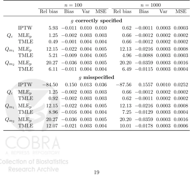
Results: Results in Table 1 confirm that all estimators are unbiased under correct parametric model specification, although sparsity in the data inflates IPTW variance at the smaller sample size. When g0 is consistently estimated,

misspecification bias in MLEp estimates that rely on specificationQm1 orQm2

is greatly reduced by the TMLE procedure. However, relative to the correctly specified MLE and IPTW estimator, some bias remains at the larger sample size. When g0 is misspecified the bias of the IPTW estimator is extreme

relative to the true parameter value (ψ0 = −0.1779), and variance is three to

four times that of MLEp and TML estimators, even when n= 1000. TMLE’s

ability to reduce the bias is impaired by misspecification of g0, but because

the submodel and quasi-log-likelihood loss function used in the estimation procedure respect the bounds on the statistical model M, the variance does not suffer(Gruber and van der Laan, 2010a).

Table 1: Simulation 1 results, ψ0 =−0.1779.

n= 100 n= 1000

Rel bias Bias Var MSE Rel bias Bias Var MSE g correctly specified IPTW 5.93 −0.011 0.010 0.010 0.62 −0.0011 0.0003 0.0003 Qc MLEp 1.25 −0.002 0.003 0.003 0.66 −0.0012 0.0002 0.0002 TMLE 0.49 −0.001 0.004 0.004 0.66 −0.0012 0.0002 0.0002 Qm1 MLEp 12.15 −0.022 0.004 0.005 12.13 −0.0216 0.0003 0.0008 TMLE 5.21 −0.009 0.004 0.005 4.96 −0.0088 0.0003 0.0003 Qm2 MLEp 20.27 −0.036 0.003 0.005 20.20 −0.0359 0.0003 0.0016 TMLE 6.11 −0.011 0.004 0.004 6.49 −0.0115 0.0003 0.0004 g misspecified IPTW −84.50 0.150 0.013 0.036 −87.56 0.1557 0.0010 0.0252 Qc MLEp 1.25 −0.002 0.003 0.003 0.66 −0.0012 0.0002 0.0002 TMLE 0.92 −0.002 0.003 0.003 0.62 −0.0011 0.0002 0.0002 Qm1 MLEp 12.15 −0.022 0.004 0.005 12.13 −0.0216 0.0003 0.0008 TMLE 8.96 −0.016 0.004 0.004 7.25 −0.0129 0.0003 0.0004 Qm2 MLEp 20.27 −0.036 0.003 0.005 20.20 −0.0359 0.0003 0.0016 TMLE 12.07 −0.021 0.003 0.004 10.01 −0.0178 0.0003 0.0006

5.2

Simulation 2: Causal effect of treatment on

sur-vival with right-censoring and time-dependent

co-variates.

Consider an observational study in which we wish to estimate the treatment-specific survival probability at time tk, ψ0 = P(T¯a > tk), where treatment

is assigned at baseline, time-dependent covariates and mortality are assessed periodically during follow-up and at the end of study. During the trial some subjects experience the event, and others drop out due to reasons related to treatment or covariate information, thereby confounding a naive effect esti-mate. The time-ordering of the intervention nodes (A), and time-dependent covariate/event nodes (L) for one such study design is shown in Figure 2.

L0 A0 A1 L1 L2 L3 A2 L4 L5 L6 A3 Y

Figure 2: Simulation 2: Time ordering of intervention and non-intervention nodes, baseline covariatesL0= (W1, W2, W3, W4, W5)), treatment nodeA0, censoring nodes

(A1, A2, A3), time-dependent covariates (L2, L3, L5, L6), intermediate and final

outcome (L1, L4, Y).

IPTW, MLEp, and TMLE were applied to 500 samples of size n1 = 100,

n2 = 1000, to estimate mean survival under treatment at time tk = 3. Data

were generated as follows:

W1, W2, W3, W4, W5 ∼N(0,1)

P(A0= 1|P a(A0)) = expit(0.1W1+ 0.2W2+ 0.1W3+ 0.2W4+ 0.1W5)

P(A1= 1|P a(A1)) = expit(0.1 + 0.2W1+ 0.4W4+ 0.2W5+ 0.1A0)

L1 = expit(−2 + 0.4W1W2+ 0.3W3+ 0.4W4−0.3W5−A0) L2 = 1 + 0.2W2+ 0.7W4+ 0.1W5+ 0.5A0+1 L3 = 1 + 0.1W1+ 0.2W3+ 0.5W5+ 0.2A0+ 0.2L2+2 P(A2= 1|P a(A2)) = expit(−0.6 + 0.3W2+A0+ 0.1L2+ 0.5L3) L4 = expit(−0.5 + 0.1W2−A0+ 0.3L2−0.7L3) L5 = 1−1.5W2+ 0.4A0 + 0.5L2+ 0.1L3+3 L6 = 1 + 0.1W3+ 2A0+ 0.6L3+ 0.2L5+4

P(A3= 1|P a(A3)) = expit(1.2−0.4A0−0.2L2+ 0.3L50.2L6)

P(Y = 1|P a(Y))) = expit(−3−0.2W1W2−0.2A0+ 0.3L3+ 0.6L5+ 0.2L6),

with1, 2, 3, 4 ∼i.i.d. N(0,1). The values of censoring nodes A(t) for subjects

set to 1 to reflect the fact that the outcome attk is known even in the absence

of additional follow-up time. The values at all nodes following censoring or an observed outcome event at time t were set to 0. As in Simulation 1, results were obtained for correct and misspecified regression models for ¯Qa

L(k) and gk.

The conditional means ¯Qq_L(k) were estimated with logistic regression models including all terms used to generate the actual data (Qc), including main term

baseline covariates only (Qm1), and an intercept-only model (Qm2). The g

factors were estimated by using correctly specified logistic regression models to regressAkon the parents ofAk, and a second time, using main terms logistic

regression models that included all covariates measured prior toAkin the time

ordering shown in Figure 2. Again, the censoring and treatment probabilities were not truncated from below.

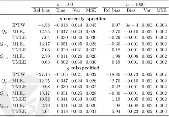
Table 2: Simulation 2,ψ0 = 0.386.

n= 100 n= 1000

Rel bias Bias Var MSE Rel bias Bias Var MSE g correctly specified IPTW −4.58 −0.018 0.044 0.045 0.07 3e−4 0.003 0.003 Qc MLEp 12.25 0.047 0.024 0.026 −2.70 −0.010 0.002 0.002 TMLE 7.64 0.030 0.030 0.030 −0.29 −0.001 0.002 0.002 Qm1 MLEp 13.17 0.051 0.025 0.028 −0.30 −0.001 0.002 0.002 TMLE 7.63 0.029 0.031 0.032 −0.18 −0.001 0.002 0.002 Qm2 MLEp 2.79 0.011 0.020 0.020 1.98 0.008 0.002 0.002 TMLE 0.63 0.002 0.030 0.030 0.19 0.001 0.002 0.002 g misspecified IPTW −27.15 −0.105 0.021 0.032 −18.80 −0.073 0.002 0.007 Qc MLEp 12.25 0.047 0.024 0.026 −2.70 −0.010 0.002 0.002 TMLE 9.98 0.039 0.030 0.032 −0.22 −0.001 0.002 0.002 Qm1 MLEp 13.17 0.051 0.025 0.028 −0.30 −0.001 0.002 0.002 TMLE 10.52 0.041 0.033 0.035 1.19 0.005 0.002 0.002 Qm2 MLEp 2.79 0.011 0.020 0.020 1.98 0.008 0.002 0.002 TMLE 4.64 0.018 0.030 0.031 5.94 0.023 0.002 0.003

Results: Sparsity in the data at small sample size increases bias in all es-timators, with the exception of TMLE under dual misspecification Qm2, gmis,

in comparison with performance at the larger sample size, where the positiv-ity assumption is met (Table 2). The G-computation estimators using the

specification Qm2 (intercept-only model) are least impacted by this violation.

Sparsity again inflates IPTW variance relative to the other estimators. When

g0 is correctly specified all estimators have comparable MSE at n = 1000. At

that sample size, if g0 is misspecified the variance dominates the MSE for all

estimators, except for the IPTW.

5.3

Inference.

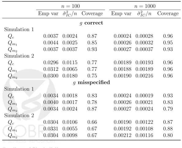
Table 3 allows us to compare the empirical variance of the Monte Carlo TMLE estimates obtained above, with influence curve-based variance esti-mates, _dvar(ψn) = ˆσIC2 /n, and lists coverage of 95% IC-based confidence

in-tervals. As an estimate of the influence curve we use the estimated efficient influence curve, which is known to be asymptotically correct if bothQ0 andg0

Table 3: Empirical variance of Monte Carlo TMLE estimates, mean IC-based variance estimates, and coverage of nominal 95% confidence intervals.

n = 100 n= 1000 Emp var ˆσ2

IC/n Coverage Emp var σˆIC2 /n Coverage

g correct Simulation 1 Qc 0.0037 0.0024 0.87 0.00024 0.00028 0.96 Qm1 0.0044 0.0025 0.85 0.00026 0.00032 0.95 Qm2 0.0037 0.0037 0.93 0.00027 0.00037 0.93 Simulation 2 Qc 0.0296 0.0115 0.77 0.00189 0.00193 0.96 Qm1 0.0312 0.0065 0.77 0.00188 0.00189 0.96 Qm2 0.0300 0.0180 0.75 0.00190 0.00216 0.96 g misspecified Simulation 1 Qc 0.0034 0.0018 0.83 0.00024 0.00019 0.93 Qm1 0.0040 0.0017 0.78 0.00026 0.00021 0.83 Qm2 0.0034 0.0024 0.87 0.00027 0.00024 0.79 Simulation 2 Qc 0.0304 0.0106 0.66 0.00190 0.00122 0.87 Qm1 0.0331 0.0055 0.67 0.00192 0.00108 0.88 Qm2 0.0304 0.0098 0.67 0.00212 0.00116 0.80

are consistently estimated, and it results in asymptotically conservative vari-ance estimates if g0 is consistently estimated. When g0 is correctly specified

sparsity in the data leads to anti-conservative confidence intervals. However when sample size is increased to 1000, observed coverage is quite close to the nominal rate. As predicted by theory, when both Q0 and g0 are misspecified,

(efficient-)influence curve-based inference is not reliable. However, ifg0 is

mis-specified but Q0 is correctly estimated, coverage is close to the nominal rate

for Simulation 1.

6

Concluding remarks.

TMLE is a general template for construction of semiparametric efficient sub-stitution estimators requiring writing the target parameter as a function of an infinite dimensional parameter (e.g., Ψ( ¯Qa)) for an infinite dimensional pa-rameter (e.g., ¯Qa), a loss function for this parameter possibly indexed by a nuisance parameter (e.g., Lη( ¯Qa)), a parametric submodel with loss

function-specific score spanning the efficient influence curve (and/or any other desired estimating function), and a specification of a resulting iterative targeted mini-mum loss-based estimation algorithm that minimizes the loss function-specific empirical risk along the parametric submodel until no further update improves the empirical risk. Since the nuisance parameters in the loss function are a function of ¯Qa_{itself, the estimator of the nuisance parameters in the loss}

func-tion are also updated at each step to reflect their last fitted value. The TMLE is a two stage procedure, where the first stage involves loss-based learning of the infinite dimensional parameter, and the subsequent stage is a targeted iterative update of this initial estimator that is only concerned with fitting the target parameter, and which guarantees that the TMLE of the infinite dimensional parameter solves the efficient influence curve equation. The in-fluence curve of the TMLE is defined by the fact that it solves this estimating equation.

As apparent from a formal analysis of the TMLE, whether the conditions for asymptotic linearity are met depends on how well (e.g., at what rate) the TMLE estimates these nuisance parameters of the efficient influence curve. The latter also affects the finite sample performance of the TMLE. Therefore, if the initial estimator of the infinite dimensional parameter in the TMLE in-volves trading off bias and variance w.r.t. an infinite dimensional parameter that is much richer than needed for evaluation of the target parameter, then finite sample performance is degraded relative to a TMLE that uses an initial estimator that involves trading off bias and variance for a smaller infinite

di-mensional parameter that is more relevant for the target parameter. From this perspective, the TMLE proposed in this article, inspired by the double robust estimator of Bang and Robins (2005), appears to be based on an excellent choice of loss function and parametric submodel.

By the same token, a substitution estimator obtained by plugging in a log-likelihood based super learner will be less targeted than a substitution estimator obtained by plugging in a loss-based super learner based on a more targeted loss function. Therefore, loss-based learning provides fundamental improvements on log-likelihood based learning by allowing the selection of a targeted loss function, and targeted minimum loss-based estimation (TMLE) provides the additional bias reduction so that the resulting estimators allow for statistical inference in terms of a central limit theorem, under appropriate regularity conditions.

It will be of interest to further evaluate the practical performance of this TMLE in future studies, in particular, in comparison with other TMLEs such as the one proposed in van der Laan (2010) and Stitelman and van der Laan (2011a) based on the log-likelihood loss function. A practical advantage of the TMLE presented in this article is that it is easier to implement since it only involves fittingK (iteratively defined) regressions, while the TMLE in van der Laan (2010) based on the log-likelihood involves fittingK conditional densities of L(K). It should be noted that by using a more targeted loss function for the initial estimator such as the one in this article, the TMLE based on fitting conditional densities can still be as good as a TMLE based on only fitting the required conditional means (see also the Appendix in van der Laan and Rose (2011) and van der Laan and Gruber (2010) for efficient influence curve based targeted loss functions that can be used to build the initial estimator). In other words, it is not a mistake to use a plug-in estimator based on an estimate of the whole density of the data, but one wants to fit this density based on a criterion for a candidate estimator that reflects the performance of the resulting plug-in estimator of the target parameter.

In this paper we made use of sequential loss-based learning defined as follows: Let Qk0 = arg minQkP0Lk,Qk+1,0(Qk) be defined as the minimizer of

the risk of a loss function that is indexed by Qk+1,0, k = K + 1, . . . ,0. Let

Q = (Q0, . . . , QK+1). The parameter of interest is a parameter Ψ(Q). For

k =K+ 1, . . . ,0, given an estimator of Qk+1,0, one applies loss-based learning

of Qk,0 based on the loss function Lk,Qk+1,0(Qk). The statistical properties

of such estimators of Q(P0) based on sequential cross-validation estimator

selection remain to be studied.

If Ψ(Q) is a pathwise differentiable parameter with efficient influence curve

proce-dure into a targeted minimum loss-based (sequential) learning algorithm: start with initial estimator Qn = (Qk,n : k = 0, . . . , K + 1) and gn, construct

sub-models {Qk(, g) : } through Qk at = 0 so that _ddLk,Qk+1(Qk(, g))

=0 = D∗_k(Q, g) and D∗(Q, g) = P kD ∗ k(Q, g), and for k = K + 1, . . . ,0, k,n =

arg minkPnLk,Q∗k+1,n(Qk,n(, gn)), where Q ∗

k,n =Qk,n(k,n). The final TMLE is

the plug-in estimator Ψ(Q∗_n), and we have PnD∗(Q∗n, gn) = 0. In particular,

the TMLE we presented in this article can be generalized to any pathwise dif-ferentiable parameter of the distribution of Ya_{, possibly conditional on L(0)}

orLa(k) at a particulark (as in history adjusted marginal structural models), by applying the conditional iterative expectation rule to (P(Ya_{=y) :a, y) as}

in this article forEYa_{, and applying the above TMLE framework with the}

de-composition of the efficient influence curve, the loss functions and submodels. Precise demonstrations for causal parameter defined by marginal structural models are presented in the Appendices below.

For future research it will also be of interest to develop a collaborative TMLE based on the TMLE presented here, thereby also allowing the targeted estimation of the intervention mechanism based on the collaborative double robustness of the efficient influence curve as presented in van der Laan and Gruber (2010) and van der Laan and Rose (2011).

APPENDIX: TMLE for causal parameters

de-fined by working MSM without baseline

covari-ates.

Consider the same longitudinal data structureO= (L(0), A(0), . . . , L(K), A(K), Y =L(K+ 1)), and statistical model M. Let La _{be the random variable with}

distribution equal to the G-computation formula Pa = QK+1

k=0 Q

a

L(k), where

Qa

L(k)is the conditional distribution ofL(k), given ¯L(k−1),A¯(k−1) = ¯a(k−1).

In this article we presented a TMLE for EYa_{. Suppose now that our target}

parameter is Ψ(Q) =f(EYa :a ∈ A) for some multivariate Euclidean valued functionf, and a collection of static regimensA. For example, given a working model {mβ :β} forEYa, and function h, we could define

Ψ(Q0) = arg min β E0 X a∈A h(a)(Ya−mβ(a))2, or if Y ∈[0,1], Ψ(Q0) = arg min β −E0 X a∈A h(a){Yalogmβ(a) + (1−Ya) log(1−mβ(a))}.

In this article we presented the efficient influence curveDa,∗ ₌P

kD a,∗

k of the

target parameter EYa _{with an orthogonal decomposition given in Theorem}

1, where D_ka,∗ is a score of the conditional distribution QL(k) of L(k), given

¯

L(k−1),A¯(k−1). The efficient influence curve of the target parameter Ψ is thus given by D∗ = P a∈Af 0 aD ∗ a, where f 0 a0 = d dEYa0f(EY a _{:a ∈ A). We note}

that this can be decomposed as

D∗ =X a f_a0 ( X k Da,_k∗ ) ≡X k D_k∗, where D_k∗ =X a f_a0D_ka,∗.

This represents an orthogonal decomposition of the efficient influence curve

D∗ of Ψ in terms of scores of QL(k). Specifically,

DK+1 = X a∈A f_a0I( ¯A(K) = a) g0:K (Y −Q¯a_K+1), and D∗_k = X a∈A f_a0I( ¯A(k−1) = ¯a(k−1)) g0:k−1 n ¯ Qa_L(k)−EQa L(k−1) ¯ Qa_L(k)o, = X a∈A f_a0I( ¯A(k−1) = ¯a(k−1)) g0:k−1 _¯ Qa_L(k)−Q¯a_L(k−1) , k=K, . . . ,0.

We note that Ψ(Q) depends on Q through ¯Q ≡ ( ¯Qa : a ∈ A), where ¯

Qa= ( ¯Qa_k=E(Ya|L¯a(k−1)) :k = 0, . . . , K+ 1). In this article we proposed a sum loss function L_a,Q¯a( ¯Qa) =

PK+1 k=0 La,k,Q¯a k+1( ¯Q a k) for ¯Qa0, where −La,k,Q¯a k+1( ¯Q a k) =I( ¯A(k−1) = ¯a(k−1)) _¯ Qa_k+1log ¯Qa_k+ (1−Q¯a_k+1) log{1−Q¯a_k} .

As a consequence, L_Q¯( ¯Q) ≡ P_a∈Af_a0L_a,Q¯a( ¯Qa) is a valid loss function for

¯ Q0 = ( ¯Qa0 :a∈ A). Note L_Q¯( ¯Q) = X a∈A f_a0 K+1 X k=0 L_a,k,Q¯a k+1( ¯Q a k) = K+1 X k=0 ( X a∈A f_a0L_a,k,Q¯a k+1( ¯Q a k) ) ≡ K+1 X k=0 Lk,Q¯k+1( ¯Qk),

where ¯Qk = ( ¯Qak : a ∈ A) and Lk,Q¯k+1( ¯Qk) = P a∈Af 0 aLa,k,Q¯a k+1( ¯Q a k) is a loss function for ¯Qk.

Consider the submodel ¯Qk(k, g) = ( ¯Qak(k, g) :a∈ A) defined by

Logit ¯Qa_L(k)(k, g) = Logit ¯QaL(k)+k

1

g0:k−1

, k=K+ 1, . . . ,0,

where we define g0:−1 = 1. This submodel does indeed satisfy the generalized

score-condition d dk Lk,Q¯k+1( ¯Qk(k, g)) k=0 =D_k∗, k = 0, . . . , K + 1.

In particular, the submodel ¯Q(0, . . . , K+1, g) defined by these k-specific

sub-models through ¯Qk,k = 0, . . . , K+ 1, and the above sum loss functionL_Q¯( ¯Q)

satisfies the condition that the generalized score spans the efficient influence curve: D∗(Q, g)∈ d dLQ¯( ¯Q(, g)) =0 . (4)

Finally, we present the TMLE-algorithm. Suppose we already obtained an initial estimator ¯Qk,n, k = 0, . . . , K + 1 and gn. Let ¯Qa,

∗ K+2,n ≡ Y for each a∈ A. For k =K+ 1 to k = 1, we compute k,n ≡arg min k PnLk,Q¯∗_k+1,n( ¯Qk,n(k, gn)),

and the corresponding update ¯Q∗_k,n = ¯Qk,n(k,n, gn). Finally, for each a ∈ A,

define ¯Qa,_L(0)∗ _,n = 1/nPn

i=1Q¯

a,∗

1,n(Li(0)), providing the TMLE ¯Q∗_L(0),nof ¯QL(0),0 =

( ¯Qa

L(0),0 :a). This defines the TMLE ¯Q

∗

n = ( ¯Q

∗

k,n, k = 0, . . . , K + 1) of ¯Q0.

Finally, we compute the TMLE ofψ0as the plug-in estimator corresponding

with ¯Q∗_n: Ψ( ¯Q∗_n) = f( ¯Q∗_L(0),n) =f 1 n n X i=1 ¯ Qa,_1,n∗(Li(0)) :a∈ A ! .

The TMLE solves the efficient influence curve equation 0 =PnD∗( ¯Qn∗, gn,Ψ( ¯Q∗n)),

thereby making it a double robust locally efficient substitution estimator, un-der regularity conditions.