A Simple Convolutional Generative Network for Next Item Recommendation

Yuan, F., Karatzoglou, A., Arapakis, I., Jose, J. M. and He, X. (2019) A Simple

Convolutional Generative Network for Next Item Recommendation. In: Twelfth

ACM International Conference on Web Search and Data Mining, Melbourne,

Australia, 11-15 Feb 2019, pp. 582-590. ISBN 9781450359405

There may be differences between this version and the published version. You are

advised to consult the publisher’s version if you wish to cite from it.

© 2019 Association for Computing Machinery. This is the author's version of the

work. It is posted here for your personal use. Not for redistribution. The definitive

Version of Record was published in WSDM '19: Proceedings of the Twelfth ACM

International Conference on Web Search and Data Mining

https://doi.org/10.1145/3289600.3290975

http://eprints.gla.ac.uk/182377/

Deposited on: 13 November 2020

Enlighten – Research publications by members of the University of Glasgow

http://eprints.gla.ac.uk

A Simple Convolutional Generative Network for Next Item

Recommendation

Fajie Yuan

Alexandros Karatzoglou

Ioannis Arapakis

Joemon M Jose

Xiangnan He

National University of Singapore Singapore

[email protected]

ABSTRACT

Convolutional Neural Networks (CNNs) have been recently intro-duced in the domain of session-based next item recommendation. An ordered collection of past items the user has interacted with in a session (or sequence) are embedded into a 2-dimensional latent matrix, and treated as an image. The convolution and pooling opera-tions are then applied to the mapped item embeddings. In this paper, we first examine the typical session-based CNN recommender and show that both the generative model and network architecture are suboptimal when modeling long-range dependencies in the item sequence. To address the issues, we introduce a simple, but very effective generative model that is capable of learning high-level representation from both short- and long-range item dependencies. The network architecture of the proposed model is formed of a stack ofholedconvolutional layers, which can efficiently increase the receptive fields without relying on the pooling operation. Another contribution is the effective use of residual block structure in recom-mender systems, which can ease the optimization for much deeper networks. The proposed generative model attains state-of-the-art accuracy with less training time in the next item recommendation task. It accordingly can be used as a powerful recommendation baseline to beat in future, especially when there are long sequences of user feedback.

ACM Reference Format:

Fajie Yuan, Alexandros Karatzoglou, Ioannis Arapakis, Joemon M Jose, and Xiangnan He. 2019. A Simple Convolutional Generative Network for Next Item Recommendation. InThe Twelfth ACM International Conference on Web Search and Data Mining (WSDM ’19), February 11–15, 2019, Melbourne,

∗_{A Part of work was done while at Telefonica Research, Spain and University of Glasgow, UK.}

Permission to make digital or hard copies of all or part of this work for personal or classroom use is granted without fee provided that copies are not made or distributed for profit or commercial advantage and that copies bear this notice and the full citation on the first page. Copyrights for components of this work owned by others than ACM must be honored. Abstracting with credit is permitted. To copy otherwise, or republish, to post on servers or to redistribute to lists, requires prior specific permission and/or a fee. Request permissions from [email protected].

WSDM ’19, February 11–15, 2019, Melbourne, VIC, Australia © 2019 Association for Computing Machinery.

ACM ISBN 978-1-4503-5940-5/19/02. . . $15.00 https://doi.org/10.1145/3289600.3290975

VIC, Australia.ACM, New York, NY, USA, 9 pages. https://doi.org/10.1145/ 3289600.3290975

1

INTRODUCTION

Leveraging sequences of user-item interactions (e.g., clicks or pur-chases) to improve real-world recommender systems has become increasingly popular in recent years. These sequences are automati-cally generated when users interact with online systems in sessions (e.g., shopping session, or music listening session). For example,

users on Last.fm1or Weishi2typically enjoy a series of songs/videos

during a certain time period without any interruptions, i.e., a lis-tening or watching session. The set of music videos played in one session usually have strong correlations [6], e.g., sharing the same album, writer, or genre. Accordingly, a good recommender system is supposed to generate recommendations by taking advantage of these sequential patterns in the session.

A class of models often employed for these sequences of interac-tions are the Recurrent Neural Networks (RNNs). RNNs typically generate a softmax output where high probabilities represent the most relevant recommendations. While effective, these RNN-based models, such as [3, 15], depend on a hidden state of the entire past that cannot fully utilize parallel computation within a sequence [8]. Thus their speed is limited in both training and evaluation.

By contrast, training CNNs does not depend on the computations of the previous time step and therefore allow parallelization over every element in a sequence. Inspired by the successful use of CNNs in image tasks, a newly proposed sequential recommender, referred

to asCaser [29], abandoned RNN structures, proposing instead

a convolutional sequence embedding model, and demonstrated that this CNN-based recommender is able to achieve comparable

or superior performance to the popular RNN model in the top-N

sequential recommendation task. The basic idea of the convolution

processing is to treat thet×kembedding matrix as the “image"

of the previoust interactions inkdimensional latent space and

regard the sequential pattens as local features of the “image". A max pooling operation that only preserves the maximum value of the convolutional layer is performed to increase the receptive field, as well as dealing with the varying length of input sequences. Fig. 1

depicts the key architecture ofCaser.

1_{https://www.last.fm} 2_{http://weishi.qq.com/}

Embedding Look-up Convolutional Layers Max pooling Fee dfo rward la ye rs t (a) (b) (c) (d)

Figure 1:The basic structure ofCaser[29]. The red, yellow and blue regions denotes a2×k,3×kand4×kconvolution filter respectively, wherek=5. The purple row stands for the true next item.

Considering the training speed of networks, in this paper we follow the path of sequential convolution techniques for the next item recommendation task. We show that the typical network

ar-chitecture used inCaserhas several obvious drawbacks — e.g.,: (1)

the max pooling scheme that is safely used in computer vision may discard important position and recurrent signals when modeling long-range sequence data; (2) generating the softmax distribution only for the desired item fails to effectively use the compete set of dependencies. Both drawbacks become more severe as the length of the sessions and sequences increases. To address these issues, we in-troduce a simple but fundamentally different CNN-based sequential recommendation model that allows us to model the complex condi-tional distributions even in very long-range item sequences. To be more specific, first our generative model is designed to explicitly encode item inter-dependencies, which allows to directly estimates the distribution of the output sequence (rather than the desired item) over the raw item sequence. Second, instead of using ineffi-cient huge filters, we stack the 1D dilated convolutional layers [31] on top of each other to increase the receptive fields when modeling long-range dependencies. The pooling layer can be safely removed in the proposed network structure. It is worth noting that although the dilated convolution was invented for dense prediction in image generation tasks [4, 26, 31], and has been applied in other fields (e.g., acoustic [22, 26] and translation [18] tasks), it is yet unexplored in recommender systems with huge sparse data. Furthermore, to ease the optimization of the deep generative architecture, we propose using residual network to wrap convolutional layer(s) by residual block. To the best of our knowledge, this is also the first work in terms of adopting residual learning to model the recommendation task. The combination of these choices enables us to tackle large-scale problems and attain state-of-the-art results in both short- and long-range sequential recommendation data sets. In summary, our main contributions include a novel recommendation generative model (Section 3.1) and a fundamentally different convolutional

network architecture (Sections 3.2∼3.4).

2

PRELIMINARIES

First, the problem of recommending items from sequences is de-scribed. Next, a recent convolutional sequence embedding

recom-mendation model (Caser) is shortly recapitulated along with its

limitations. Lastly, we review previous work on sequence-based recommender systems.

2.1

Top-

N

Session-based Recommendation

Let{x0,x1, ...,xt−1,xt}(interchangeably denoted byx0:t) be an

user-item interaction sequence (or a session), wherexi ∈R(0≤i≤

t)is the index of the clicked item out of a total number oft+1 items

in the sequence. The goal of sequential recommendation is to seek

a model such that for a given prefix item sequence,x={x0, ...,xi}

(0≤i<t), it generates a ranking or classification distributionyfor

all candidate items, wherey=[y1, ...,yn] ∈Rn.yjcan be a score,

probability or a rank of itemi+1 that will occur in this sequence.

In practice, we typically make more than one recommendation by

choosing the top-N items fromy, referred to as the top-N

session-based (sequential) recommendations.

2.2

Limitations of

Caser

The basic idea ofCaseris to embed the previoustitems as at×k

matrixEby the embedding look-up operation, as shown in Fig. 1 (a).

Each row vector of the matrix corresponds to the latent features of one item. The embedding matrix can be regarded as the “image" of

thetitems in thek-dimensional latent space. Intuitively, models

of various CNNs that are successfully applied in computer vision can be adapted to model the “image" of an item sequence. How-ever, there are two aspects that differentiate sequence modeling from image processing, which makes the use of CNN based models non-straightforward. First, the variable-length item sequences in real-world scenarios produce a large number of “images" of differ-ent sizes, where traditional convolutional structures with fix-sized filters may fail. Second, the most effective filters for images, such as

3×3 and 5×5, are not suitable for sequence “images" since these

small filters (in terms of row-wise orientation) are not suitable to capture the representations of full-width embedding vectors.

To address the above limitations, filters inCaserslide over full

columns of the sequence “image” by large filter. That is, the width of filters is usually the same as the width of the input “images". The

height typically varies by sliding windows over 2−5 items at a time

(Fig. 1 (a)). Filters of different sizes will generate variable-length feature maps after convolution (Fig. 1 (b)). To ensure that all maps have the same size, the max pooling is performed over each map, which selects only the largest number of each feature map, resulting

in a 1×1 map (Fig. 1 (c)). Finally, these 1×1 maps from all filters

are concatenated to form a feature vector, followed by a softmax layer that yields the probabilities of next item (Fig. 1 (d)). Note that we have omitted the vertical convolution in Fig. 1, since it does not solve the major problems discussed below.

Based on the above analysis of the convolutions inCaser, one

may find that there exist several drawbacks with the current design. First, the max pooling operator has obvious disadvantages. It cannot distinguish whether an important feature in the map occurs just one or multiple times and it ignores the position in which it occurs. The max pooling operator while safely used in image processing

(with small pooling filters, e.g., 3×3) may be harmful for modeling

long-range sequences (with large filters, e.g., 1×20). Second, the

convolutional layer is likely to fail when modeling complex rela-tions or long-range dependences. The last important disadvantage comes from the generative process of next item, which we will describe in detail in Section 3.1.

2.3

Related Work

Early work in sequential recommendations mostly rely on the markov chain [5] and feature-based matrix factorization [12, 32–34] approaches. Compared with neural network models, the markov chain based approaches fail to model complicated relations in the

se-quence data. For example, inCaser, the authors showed that markov

chain approaches failed to model union-level sequential patterns and did not allow skip behaviors in the item sequences. Factor-ization based approaches such as factorFactor-ization machines model a sequence by the sum of its item vectors. However, these methods do not consider the order of items and are not specifically invented for sequential recommendations.

Recently, deep learning models have shown state-of-the-art rec-ommendation accuracy in contrast to conventional models. More-over, RNNs, a class of deep neural networks, have almost dominated the area of sequential recommendations. For example, a Gated

Re-current Unit (GRURec) architecture with a ranking loss was

pro-posed by [15] for session-based recommendation. In the follow-up papers, various RNN variants have been designed to extend the typical one for different application scenarios, such as by adding personalization [25], content [9] and contextual features [27], at-tention mechanism [7, 20] and different ranking loss functions [14]. By contrast, CNN based sequential recommendation models are more challenging and much less explored because convolutions are not a natural way to capture sequential patterns. To our best knowledge, only two types of sequential recommendation

archi-tectures have been proposed to date: the first one byCaseris a

standard 2D CNN, while the second is a 3D CNN [30] designed to model high-dimensional features. Unlike the aforementioned examples, we plan to investigate the effects of 1D CNNs with ef-ficient dilated convolution filters and residual blocks for building the recommendation architecture.

3

MODEL DESIGN

To address the above limitations, we introduce a new probabilistic generative model that is formed of a stack of 1D convolution layers. We first focus on the form of the distribution, and then the architec-tural innovations. Generally, our proposed model is fundamentally

different fromCaserin several key ways: (1) our probability

esti-mator explicitly models the distribution transition of all individual items at once, rather than the final one, in the sequence; (2) our network has a deep, rather than shallow, structure; (3) our convo-lutional layers are based on the efficient 1D dilated convolution rather than standard 2D convolution; and (4) pooling layers are removed.

3.1

A Simple Generative Model

In this section, we introduce a simple yet very effective generative model directly operating on the sequence of previous interacted items. Our aim is to estimate a distribution over the original item

interaction sequences that can be used totractablycompute the

likelihood of the items and to generate the future items that users

would like to interact. Letp(x)be the joint distribution of item

sequencex={x0, ...,xt}. To modelp(x), we can factorize it as a

product of conditional distributions by the chain rule. p(x)=

t

Ö

i=1

p(xi|x0:i−1,θ)p(x0) (1)

where the valuep(xi|x0:i−1,θ)is the probability ofi-th itemxi

conditioned on all the previous itemsx0:i−1. A similar setup has

been explored by NADE [19], PixelRNN/CNN [23, 24] in biological and image domains.

Owing to the ability of neural networks in modeling complex nonlinear relations, in this paper we model the conditional distribu-tions of user-item interacdistribu-tions by a stack of 1D convolutional

net-works. To be more specific, the network receivesx0:t−1as the input

and outputs distributions over possiblex1:t, where the distribution

ofxtis our final expectation. For example, as illustrated in Fig. 2, the

output distribution ofx15is determined byx0:14, whilex14is

deter-mined byx0:13. It is worth noting that in previous sequential

recom-mendation literatures, such asCaser,GRURecand [20, 25, 28, 30],

they only model a single conditional distributionp(xi|x0:i−1,θ)

rather than all conditional probabilitiesÎt

i=1p(xi|x0:i−1,θ)p(x0).

Within the context of the above example, assuming{x0, ...,x14}

is given, models likeCaseronly estimate the probability

distribu-tion (i.e., softmax) of the next itemx15(also see Fig. 1 (d)), while

our generative method estimates the distributions of all individual

items in{x1, ...,x15}. The comparison of the generating process is

shown below.

Caser/GRU Rec:{x0,x1, ...,x14}

| {z } input ⇒ x15 |{z} output Ours:{x0,x1, ...,x14} | {z } input ⇒ {x1,x2, ...,x15} | {z } output (2)

where⇒denotes ‘predict’. Clearly, our proposed model is more

effective in capturing the set of all sequence relations, whereas

CaserandGRURecfail toexplicitlymodel the internal sequence

features between{x0, ...,x14}. In practice, to address the drawback,

such models will typically generate a number of sub-sequences (or sub-sessions) for training by means of data augmentation tech-niques [28] (e.g., padding, splitting or shifting the input sequence), such as shown in Eq. (3) ( see [20, 25, 29, 30]).

Caser/GRU Rec sub−session−1 :{x−1,x0, ...,x13} ⇒x14 Caser/GRU Rec sub−session−2 :{x−1,x−1, ...,x12} ⇒x13

...

Caser/GRU Rec sub−session−12 :{x−1,x−1, ...,x2} ⇒x3 (3)

While effective, the above approach to generate sub-session cannot guarantee the optimal results due to the separate optimization for each sub-session. In addition, optimizing these sub-sessions sepa-rately will result in corresponding computational costs. Detailed comparison with empirical results has also been reported in our experimental sections.

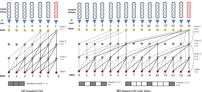
Input Conv:1 r=3 Conv:2 r=5 Conv:3 r=7 item 0 1 2 3 4 5 6 1 2 3 4 5 6 7 item Standard Conv1D 1×3 Sampled Softmax FC Layer (a)Standard CNN item 0 1 2 3 4 5 6 7 8 9 10 11 12 13 14 1 2 3 4 5 6 7 8 9 10 11 12 13 14 15 item Conv1D: 1×3 𝑙=2 Conv1D: 1𝑙=4 ×3 Sampled Softmax FC Layer Input 𝑙=1 Conv:1 𝑙=2 r=3 Conv:2 𝑙=4 r=7 Conv:3 𝑙=8 r=15

(b)Dilated CNN with ‘Holes’

Figure 2:The proposed generative architecture with 1D standard CNNs (a) and efficient dilated CNNs (b). The blue lines are the identity map which exists only for residual block (b) in Fig. 3. An example of a standard 1D convolution filter and dilated filters are shown at the bottom of (a) and (b) respectively. We will refer to a dilated convolution with a dilation factorlasl-dilated convolution. Apparently, compared with the standard CNN that linearly increases the receptive field by the depth of the network, the dilated CNN has a much larger receptive field by the same stacks without introducing more parameters. It can be seen that the standard convolution is a special case of 1-dilated convolution.

3.2

Network Architecture

3.2.1 Embedding Look-up Layer:Given an item sequence{x0, ...,xt},

the model retrieves each of the firsttitems{x0, ...,xt−1}via a

look-up table, and stacks these item embeddings together. Assuming

the embedding dimension is 2k, wherekcan be set as the number

of inner channels in the convolutional network. This results in a

matrix of sizet×2k. Note that unlikeCaserthat treats the input

matrix as a 2D “image" during convolution, our proposed architec-ture learns the embedding layer by 1D convolutional filters, which we will describe later.

3.2.2 Dilated layer: As shown in Fig. 2 (a), the standard filter is

only able to perform convolution with the receptive field linearly by the depth of the network. This makes it difficult to handle long-range sequences. Similar to Wavenet [22], we employ the dilated convolution to construct the proposed generative model. The basic idea of dilation is to apply the convolutional filter over a field larger than its original length by dilating it with zeros. As such, it is more efficient since it utilizes fewer parameters. For this reason, a dilated

filter is also referred to as aholedorsparsefilter. Another benefit is

that dilated convolution can preserve the spatial dimensions of the input, which makes the stacking operation much easier for both convolutional layers and residual structures.

Fig. 2 shows the network comparison between the standard con-volution and dilated concon-volutions with the proposed sequential

generative model. The dilation factor in (b) are 1,2,4 and 8. To

describe the network architecture, we denote receptive field,j-th

convolutional layer, channel and dilation asr,Fj,Candl

respec-tively. By setting the width of convolutional filterf as 3, we can

see that the dilated convolutions (Fig. 2 (b)) allow for exponential

increase in the size of receptive fields (r=2j+1−1), while the same

stacking structure for the standard convolution (Fig. 2 (a)) has only

linear receptive fields (r =2j+1). Formally, with dilationl, the

filter window from locationiis given as

h

xi xi+l xi+2l ... xi+(f−1)·l

i

and the 1D dilated convolution operator∗_lon elementhof the item

sequence is given below

(x∗_lд)(h)=

f−1

Õ

i=0

xh−l·i·д(i) (4)

whereдis the filter function. Clearly, the dilated convolutional

structure is more effective to model long-range item sequences, and thus more efficient without using larger filters or becoming deeper. In practice, to further increase the model capacity and receptive fields, one just need to repeat the architecture in Fig. 2 multiple times by stacking, e.g., 1,2,4,8,1,2,4,8.

3.2.3 One-dimensional Transformation:Although our dilated

con-volution operator depends on the 2D input matrixE, the proposed

network architecture is actually composed of all 1D convolutional layers. To model the 2D embedding input, we perform a simple reshape operation, which serves as a prerequisite for performing

1D convolution. Specifically, the 2D matrixEis reshaped fromt×2k

to a 3D tensorTof size 1×t×2k, where 2kis treated as the “image”

channel rather than the width of the standard convolution filter in

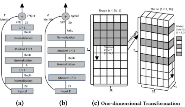
1×1 + Masked 1×3 Normalization ReLU Input E Normalization 1×1 Normalization 2𝑘 E identity F(E)+E F(E) 2𝑘 𝑘 ReLU ReLU (a) + Masked 1×3 Normalization ReLU Input E Masked 1×3 2𝑘 E identity F(E)+E F(E) 2𝑘 ReLU Normalization (b) t Dilated Conv1D： (1×3, 2k) 2k t Shape (t×2k, 1) Standard Conv2D (3×2k,1) 1 Shape (1×t, 2k) (c)One-dimensional Transformation

Figure 3:Dilated residual blocks (a), (b) and one-dimensional trans-formation (c). (c) shows the transtrans-formation from the 2D filter (C= 1)(left) to the 1D 2-dilated filter (C =2k) (right); the vertical black arrows represent the direction of the sliding convolution. In this work, the default stride for the dilated convolution is 1. Note the re-shape operation in (b) is performed before each convolution in (a) and (b) (i.e.,1×1and masked1×3), which is then followed by a reshape back step after convolution.

3.3

Masked Convolutional Residual Network

Although increasing the depth of network layers can help obtain higher-level feature representations, it also easily results in the vanishing gradient issue, which makes the learning process much harder. To address the degradation problem, residual learning [10] has been introduced for deep networks. While residual learning has achieved huge success in the domain of computer vision, it has not appeared in the recommender system literature.

The basic idea of residual learning is to stack multiple convolu-tional layers together as a block and then employ a skip connection scheme that passes the previous layers’s feature information to its posterior layer. The skip connection scheme allows to explicitly fit the residual mapping rather than the original identity mapping, which can maintain the input information and thus enlarge the

prop-agated gradients. Formally, denoting the desired mapping asH(E),

we let the residual block fit another mapping ofF(E)=H(E) −E.

The desired mapping now is recast intoF(E)+Eby element-wise

addition (assuming thatF(E)andEare of the same dimension).

As has been evidenced in [10], optimizing the residual mapping

F(E)is much easier than the original, unreferenced mappingH(E).

Inspired by [11, 18], we introduce two residual modules in Fig. 3 (a) and (b).

In (a), we wrap each dilated convolutional layer by a residual block, while in (b) we wrap every two dilated layers by a different residual block. That is, with the design of block (b), the input layer and the second convolutional layer should be connected by skip connection (i.e., the blue lines in Fig. 2). Specifically, each block is made up of the normalization, activation (e.g., ReLU [21]), con-volutional layers and a skip connection in a specific order. In this work we adopt the state-of-the-art layer normalization [1] before each activation layer, as it is well suited to sequence processing and online learning in contrast with batch normalization [16].

Regarding the properties of the two residual networks, the resid-ual block in (a) consists of 3 convolution filters: one dilated filter of

size 1×3 and two regular filters of size 1×1. The 1×1 filters are

introduced to change the size ofCso as to reduce the parameters

to be learned by the 1×3 kernel. The first 1×1 filter (close to input

Ein Fig. 3 (a)) is to changeCfrom 2ktok, while the second 1×1

filter does the opposite transformation in order to maintain the spatial dimensions for the next stacking operation. To show the

effectiveness of the 1×1 filters in (a), we compute the number of

parameters in both (a) and (b). For simplicity, we omit the activation and normalization layers. As we can see, the number of parameters

for the 1×3 filter is 1×3×2k×2k=12k2(i.e., in (b)) without the

1×1 filters. While in (a), the number of parameters to be learned is

1×1×2k×k+1×3×k×k+1×1×k×2k=7k2. The residual

mappingF(E,{Wi})in (a) and (b) is formulated as:

F(E,{Wi})=

(

W3(σ(ψ(W2(σ(ψ(W1(σ(ψ(E)))))))))) Fig.3 (a)

σ(ψ(W₄′(σ(ψ(W₂′(E))))) Fig.3 (b)

(5)

whereσandψdenote ReLU and layer-normalization,W1andW3

denote the convolution weight function of standard 1×1

convolu-tions, andW2,W₂′andW₄′denote the weight function ofl-dilated

convolution filter with size of 1×3. Note that bias terms are omitted

for simplifying notations.

3.3.1 Dropout-mask:To avoid the future information leakage

prob-lem, we propose a masking-based dropout trick for the 1D dilated convolution to prevent the network from seeing the future items.

Specifically, when predictingp(xi|x0:i−1), the convolution filters

are not allowed to make use of the information fromxi:t. Fig. 4

shows several different ways to perform convolution. As shown, our dropout-masking operation can be implemented either by padding the input sequence in (d) or shifting the output sequence by a few timesteps in (e). The padding method in (e) is very likely to result in information loss in a sequence, particularly for short sequences. Hence in this work, we apply the padding strategy in (d) with the

padding size of(f −1) ∗l.

3.4

Final Layer, Network Training and

Generating

As mentioned, the matrix in the last layer of the convolution

archi-tecture (see Fig. 2), denoted byEo, preserves the same dimensional

size of the inputE, i.e.,Eo ∈Rt×2k. However, the output should be

a matrix or tensor that contains probability distributions of all items

in the output sequencex1:t, where the probability distribution of

xt is the desired one that generates top-Npredictions. To do this,

we can simply use one more convolutional layer on top of the last

convolutional layer in Fig. 2 with filter of size 1×1×2k×n, wheren

is the number of items. Following the procedure of one-dimensional transformation in Fig. 3 (c), we obtain the expected ouput matrix

Ep _∈

Rt×n, where each row vector after the softmax operation

represents the categorical distribution overxi(0<i≤t).

The aim of optimization is to maximize the log-likelihood of the

training data w.r.t.θ. Clearly, maximizing logp(x)is mathematically

equivalent to minimizing thesumof the binary cross-entropy loss

for each item inx1:t. For practical recommender systems with tens

of millions items, the negative sampling strategy can be applied to bypasses the generation of full softmax distributions, where

the 1×1 convolutional layer is replaced by a fully-connected (FC)

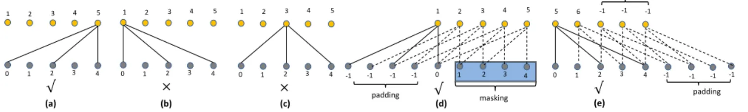
0 1 2 3 4 1 2 3 4 5 √ 0 1 2 3 4 1 2 3 4 5 × 3 0 1 2 4 1 2 3 4 5 × 0 1 2 3 4 1 2 3 4 5 √ -1 -1 -1 -1 padding _masking (a) (b) (c) (d) -1 padding 3 0 1 2 4 5 6 -1 -1 -1 √ (e) -1 -1 -1 padding

Figure 4:The future item can only be determined by the past ones according to Eq. (1). (a) (d) and (e) show the correct convolution process, while (b) and (c) are wrong. E.g., in (d), items of{1,2,3,4}are masked when predicting1, which can be technically implemented by padding.

either the sampled softmax [17] or kernel based sampling [2]. The recommendation accuracy by these negative sampling strategies is nearly identical with the full softmax method with properly tuned sampling size.

For comparison purpose, we only predict the next one item in our evaluation, and then stop the generating process. Nevertheless, the model is able to generate a sequence of items simply by feeding the predicted one item (or sequence) into the network to predict

the next one, and thus the prediction at the generating phrase is

se-quential. This matches most real-world recommendation scenarios, where the next action is followed when the current one has been observed. But at both training and evaluation phases, the

condi-tional predictions for all timesteps can be madein parallel, because

the complete sequence of input itemsxis already available.

4

EXPERIMENTS

In this section we detail our experiments, report results for several

data sets, and compare our model (calledNextItNet) with the

well-known RNN-based modelGRURec[15, 28] and the state-of-the-art

CNN-based modelCaser. Note that (1) since the main contributions

in this paper do not focus on combining various features, we omit the comparison with content- or context-based sequential recom-mendation models, such as the 3D CNN recommender [30] and

other RNN variants [9, 20, 25, 27]; (2) theGRURecbaseline could

be regarded as the state-of-the-artImproved GRURec[28] when

dealing with the long-range session data sets because our main data augmentation technique for the two baseline models follows

the same way inImproved GRURec.

4.1

Datasets and Experiment Setup

4.1.1 Datasets and Preprocessing. The first data set

‘Yoochoose-buys’ (YOO for short) is chosen from the RecSys Challenge 20153.

We use the buying dataset for evaluation. For preprocessing, we filter out sessions of length shorter than 3. Meanwhile, we find that in the processed Yoo data 96% sessions have a length shorter than 10, and we simply remove the 4% longer sessions and refer it as a short-range sequential data.

The remaining data sets are extracted from Last.fm4: one

medium-size (MUSIC_M) and one large-scale (MUSIC_L) collection by

ran-domly drawing 20,000 and 200,000 songs respectively. In the Last.fm data set, we observe that most users listen to music several hundred times a week, and some even listen to more than one hundred songs 3_{http://2015.recsyschallenge.com/challenge.html}

4_{http://www.dtic.upf.edu/ ocelma/MusicRecommendationDataset/lastfm-1K.html}

within a day. Hence, we are able to test our model in both short-and long-range sequences by cutting up these long-range listening

sessions. InMUSIC_L, we define the maximum session lengthtas

5, 10, 20, 50 and 100, and then extract everytsuccessive items as

our input sequences. This is done by sliding a window of both size

and stride oftover the whole data. We ignore sessions in which

the time span between the last two items is longer than 2 hours.

In this way, we create 5 data sets, referred to asRAW-SESSIONS.

We randomly split theseRAW-SESSIONSdata into training (50%),

validation (5%), and testing (45%) sets.

As mentioned before, the performance ofCaserandGRURecis

supposed to degrade significantly for long sequence inputs, such

as whent = 20, 50 and 100. For example, when settingt =50,

CaserandGRURecwill predictx49by usingx0:48, but without

ex-plicitly modeling the item inter-dependencies betweenx0andx48.

To remedy this defect, whent >5, we follow the common approach

[20, 28] by manually creating additional sessions from thetraining

sets ofRAW-SESSIONSso thatCaserandGRUReccan leverage the

full dependency to a large extent. Still settingt =50, one

train-ing session will then produce 45 more sub-sessions by paddtrain-ing

the beginning and removing the end indices, referred to as

SUB-SESSIONS. The example of the 45 sub-sessions are given as follows: {x−1,x0,x1, ...,x48},{x−1,x−1,x0, ...,x47},...,{x−1,x−1,x−1, ...,x4}.

RegardingMUSIC_M, we only show the results whent =5. We

show the statistics ofRAW-SESSIONS& training data ofSUB-SESSIONS

(i.e.,SUB-SESSIONS-T) in Table 1.

All models were trained on GPUs (TITAN V) using Tensorflow. The learning rates and batch sizes of baseline methods were man-ually set according to performance in validation sets. For all data

sets,NextItNet used the learning rate of 0.001 and batch size of

32. Embedding size 2kis set to 64 for all models without special

mention. We report results with residual block (a) and full softmax. We have validated the performance of results block (b) separately. To further evaluate the effectiveness of the two residual blocks, we

have also tested our model in another dataset, namely, Weishi5. The

improvements are about two times compared with the same model without residual blocks.

4.1.2 Evaluation Protocols.We reported the evaluated results by

three popular top-Nmetrics, namely MRR@N(Mean Reciprocal

Rank) [15], HR@N(Hit Ratio) [13] and NDCG@N[34] (Normalized

Discounted Cumulative Gain).N is set to 5 and 20 for comparison.

We evaluate the prediction accuracy of thelast(i.e., next) item of

each sequence in the testing set, similarly to [14]. 5_{We are working to release this dataset, which has very good sequential property.}

Table 1:Session statistics of all data sets.

DATA YOO MUSIC_M5 MUSIC_L5 MUSIC_L10 MUSIC_L20 MUSIC_L50 MUSIC_L100

RAW-SESSIONS 0.14M 0.61M 2.14M 1.07M 0.53M 0.21M 0.11M

SUB-SESSIONS-T 0.07M 0.31M 1.07M 3.21M 4.28M 4.91M 5.10M

MUSIC_M5denotesMUSIC_Mwith maximum session size of5. The same applies toMUSIC_L. ‘M’ denotes 1 million.

Table 2:Accuracy comparison. The upper, middle and below tables are MRR@5, HR@5and NDCG@5respectively.

DATA YOO MUSIC_M5 MUSIC_L5 MUSIC_L10 MUSIC_L20 MUSIC_L50 MUSIC_L100

MostPop 0.0050 0.0024 0.0006 0.0007 0.0008 0.0007 0.0007 GRURec 0.1645 0.3019 0.2184 0.2124 0.2327 0.2067 0.2086 Caser 0.1523 0.2920 0.2207 0.2214 0.1947 0.2060 0.2080 NextItNet 0.1715 0.3133 0.2327 0.2596 0.2748 0.2735 0.2583 MostPop 0.0151 0.0054 0.0014 0.0016 0.0016 0.0016 0.0016 GRURec 0.2773 0.3610 0.2626 0.2660 0.2694 0.2589 0.2593 Caser 0.2389 0.3368 0.2443 0.2631 0.2433 0.2572 0.2588 NextItNet 0.2871 0.3754 0.2695 0.3014 0.3166 0.3218 0.3067 MostPop 0.0075 0.0031 0.0008 0.0009 0.0010 0.0009 0.0009 GRURec 0.1923 0.3166 0.2294 0.2258 0.2419 0.2197 0.2212 Caser 0.1738 0.3032 0.2267 0.2318 0.2068 0.2188 0.2207 NextItNet 0.2001 0.3288 0.2419 0.2700 0.2853 0.2855 0.2704

MostPopreturns the most popular item respectively. Regarding the setup of our model, we use two-hidden-layer convolution structure with dilation factor1,2,4for the first four data sets (i.e.,YOO,MUSIC_M5,MUSIC_L5andMUSIC_L10), while for the last three long-range sequence data sets, we use1,2,4,8,1,2,4,8,to obtain above results.

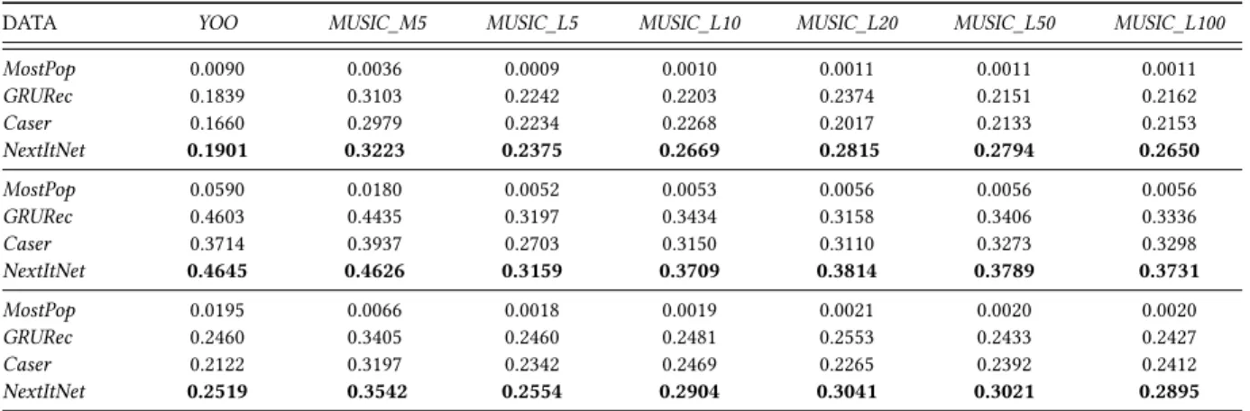
Table 3:Accuracy comparison. The upper, middle and below tables are MRR@20, HR@20and NDCG@20respectively.

DATA YOO MUSIC_M5 MUSIC_L5 MUSIC_L10 MUSIC_L20 MUSIC_L50 MUSIC_L100

MostPop 0.0090 0.0036 0.0009 0.0010 0.0011 0.0011 0.0011 GRURec 0.1839 0.3103 0.2242 0.2203 0.2374 0.2151 0.2162 Caser 0.1660 0.2979 0.2234 0.2268 0.2017 0.2133 0.2153 NextItNet 0.1901 0.3223 0.2375 0.2669 0.2815 0.2794 0.2650 MostPop 0.0590 0.0180 0.0052 0.0053 0.0056 0.0056 0.0056 GRURec 0.4603 0.4435 0.3197 0.3434 0.3158 0.3406 0.3336 Caser 0.3714 0.3937 0.2703 0.3150 0.3110 0.3273 0.3298 NextItNet 0.4645 0.4626 0.3159 0.3709 0.3814 0.3789 0.3731 MostPop 0.0195 0.0066 0.0018 0.0019 0.0021 0.0020 0.0020 GRURec 0.2460 0.3405 0.2460 0.2481 0.2553 0.2433 0.2427 Caser 0.2122 0.3197 0.2342 0.2469 0.2265 0.2392 0.2412 NextItNet 0.2519 0.3542 0.2554 0.2904 0.3041 0.3021 0.2895

Table 4:Effects of sub-session in terms of MRR@5. The upper, mid-dle and below tables represent GRU, Caser and NextItNet respec-tively. “10”,“20”,“50” and “100” are the session lengths.

Sub-session 10 20 50 100 Without 0.1985 0.1645 0.1185 0.0746 With 0.2124 0.2327 0.2067 0.2086 Without 0.1571 0.1012 0.0216 0.0084 With 0.2214 0.1947 0.2060 0.2080 Without 0.2596 0.2748 0.2735 0.2583

Table 5:Effects of the residual block in terms of MRR@5. “ With-out” means no skip connection. “M5”, “L5”, “L10” and “L50” denote

MUSIC_M5,MUSIC_L5,MUSIC_L10andMUSIC_L50 respectively.

DATA M5 L5 L10 L50

Without 0.2968 0.2146 0.2292 0.2432

With 0.3300 0.2455 0.2645 0.2760

4.2

Results Summary

Overall performance results of all methods are illustrated in Ta-ble 2 and 3, which clearly show that the neural network models

(i.e.,Caser,GRURecand our model) obtain very promising

Table 6:Effects (MRR@5) of increasing embedding size. The upper and below tables areMUSIC_M5 andMUSIC_L100 respectively.

2k 16 32 64 128 GRURec 0.2786 0.2955 0.3019 0.3001 Caser 0.2855 0.2982 0.2979 0.2958 NextItNet 0.2793 0.3063 0.3133 0.3183 GRURec 0.1523 0.1826 0.2086 0.2043 Caser 0.0643 0.1129 0.2080 0.2339 NextItNet 0.1668 0.2289 0.2583 0.2520

MUSIC_M5, the three neural models perform more than 120 times

better on MRR@5 thanMostPop, which is a widely used

recommen-dation benchmark. The best MRR@20 result we have achieved by

NextItNetis 0.3223 in this data set, which roughly means that the desired item is ranked on position 3 in average among the 20,000 candidate items. We then find that among these neural network

based models,NextItNetlargely outperformsCaser&GRURec. We

believe there are several reasons contributing to the state-of-the-art

results. First, as highlighted in Section 3.1,NextItNettakes full

ad-vantage of the complete sequential information. This can be easily

verified in Table 4, where we observe thatCaser&GRURecwithout

subsession perform extremely worse with long sessions. In

addi-tion, even with sub-sessionCaser&GRURecstill show significantly

worse results thanNextItNetbecause the separate optimization of

each sub-session is clearly suboptimal compared with leveraging

full sessions byNextItNet. Second, unlikeCaser,NextItNethas no

pooling layers, although it is also a CNN based model. As a result,

NextItNetpreserves the whole spatial resolution of the original

embedding matrixEwithout any information lost. The third

advan-tage is thatNextItNetcan support deeper layers by using residual

learning, which better suits for modeling complicated relations and long-range dependencies. We have separately validated the performance of residual block in Fig. 3 (b) and showed the results

in Table 5. It can be observed that the performance ofNextItNet

can be significantly improved by the residual block design. Table 6 shows the impact of embedding sizes.

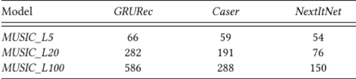
In addition to the advantage of recommendation accuracy, we

have also evaluated the efficiency ofNextItNetin Table 7. First, it

can be seen thatNextItNetandCaserrequires less training time than

GRURecin all three data sets. The reason that CNN-based models can be trained much faster is due to the full parallel mechanism of convolutions. Clearly, the training speed advantage of CNN models are more preferred by modern parallel computing systems. Second,

it shows thatNextItNetachieves further improvements in training

time compared withCaser. The faster training speed is mainly

becauseNextItNetleverages the complete sequential information

during training and then converges much faster by less training epochs. To better understand of the convergence behaviours, we have shown them in Fig. 5. As can be seen, our model with the same number of training sessions converges faster (a) and better

(b, c, d) thanCaserandGRURec. This confirms our claim in Section

3.1 sinceCaserandGRUReccannot make full use of the internal

sequential information in the session.

Table 7:Overall training time (mins).

Model GRURec Caser NextItNet

MUSIC_L5 66 59 54

MUSIC_L20 282 191 76

MUSIC_L100 586 288 150

5

CONCLUSION

In this paper, we presented a simple, efficient and highly effective

convolutional generative model for session-based top-Nitem

rec-ommendations. The proposed model combines masked filters with 1D dilated convolutions to increase the receptive fields, which is very important to model the long-range dependencies. In addition, we have applied residual learning to enable training of much deeper networks. We have shown that our model can greatly outperform state-of-the-arts in real-world session-based recommendation tasks. The proposed model can serve as a generic method for modeling both short- and long-range session-based recommendation data.

For comparison purposes, we have not considered additional contexts in either our model or baselines. However, our model is flexible to incorporate various context information. For example,

if we know the user identityuand locationp, the distribution in

Eq. (1) can be modified as follows to incorporate these information. p(x)=

t

Ö

i=1

p(x_i|x0:i−1,u,P,θ)p(x0) (6)

where we can combineE (before convolution) orEo(after

con-volution) with the user embedding vectoruand location matrix

Pby element-wise operations, such as multiplication, addition or

concatenation. We leave the evaluation for future work.

ACKNOWLEDGMENTS

This paper was supported by the European Union’s Horizon 2020 Re-search and Innovation program under grant agreement No 780787.

REFERENCES

[1] Jimmy Lei Ba, Jamie Ryan Kiros, and Geoffrey E Hinton. 2016. Layer normalization.arXiv preprint arXiv:1607.06450(2016).

[2] Guy Blanc and Steffen Rendle. 2017. Adaptive Sampled Softmax with Kernel Based Sampling.arXiv preprint arXiv:1712.00527(2017). [3] Sotirios P. Chatzis, Panayiotis Christodoulou, and Andreas S. Andreou.

2017. Recurrent Latent Variable Networks for Session-Based Recom-mendation. InProceedings of the 2nd Workshop on Deep Learning for Recommender Systems (DLRS 2017). ACM, 38–45.

[4] Liang-Chieh Chen, George Papandreou, Iasonas Kokkinos, Kevin Mur-phy, and Alan L Yuille. 2016. Deeplab: Semantic image segmentation with deep convolutional nets, atrous convolution, and fully connected crfs.arXiv preprint arXiv:1606.00915(2016).

[5] Chen Cheng, Haiqin Yang, Michael R Lyu, and Irwin King. 2013. Where You Like to Go Next: Successive Point-of-Interest Recommendation.. InIJCAI.

[6] Zhiyong Cheng, Jialie Shen, Lei Zhu, Mohan Kankanhalli, and Liqiang Nie. 2017. Exploiting Music Play Sequence for Music Recommendation. InIJCAI.

[7] Qiang Cui, Shu Wu, Yan Huang, and Liang Wang. 2017. A Hierarchical Contextual Attention-based GRU Network for Sequential Recommen-dation.arXiv preprint arXiv:1711.05114(2017).

0 2 4 6 8 10 12 14 4 6 8 10 12 training instances

Avg loss NextItNet g=256k

Caser g=256k GRU g=256k (a)Loss 0 2 4 6 8 10 12 14 0 0.08 0.16 0.24 training instances MRR@100 NextItNet g=256k Caser g=256k GRU g=256k (b)MRR@5 0 2 4 6 8 10 12 14 0 0.1 0.2 0.3 training instances HR@100 NextItNet g=256k Caser g=256k GRU g=256k (c)HR@5 0 2 4 6 8 10 12 14 0 0.08 0.16 0.24 0.32 training instances NDCG@100 NextItNet g=256k_{Caser g=256k} GRU g=256k (d)NDCG@5

Figure 5:Convergence behaviors ofMUSIC_L100.GRUis short forGRURec.д=256k means the number of training sequences (or sessions) of one unit in x-axis is 256k. Note that (1) to speed up the experiments, all of the convergence tests are evaluated on the first 1024 sessions in the testing set; (2) onlyNextItNethas converged in above figures, whileGRUandCaserrequire more training instances for convergence.

[8] Jonas Gehring, Michael Auli, David Grangier, Denis Yarats, and Yann N Dauphin. 2017. Convolutional Sequence to Sequence Learning.arXiv preprint arXiv:1705.03122(2017).

[9] Youyang Gu, Tao Lei, Regina Barzilay, and Tommi S Jaakkola. 2016. Learning to refine text based recommendations.. InEMNLP. 2103–2108. [10] Kaiming He, Xiangyu Zhang, Shaoqing Ren, and Jian Sun. 2016. Deep

residual learning for image recognition. InCVPR. 770–778.

[11] Kaiming He, Xiangyu Zhang, Shaoqing Ren, and Jian Sun. 2016. Iden-tity mappings in deep residual networks. InECCV. Springer, 630–645. [12] Xiangnan He and Tat-Seng Chua. 2017. Neural factorization machines

for sparse predictive analytics. InSIGIR. ACM, 355–364.

[13] Xiangnan He, Zhankui He, Xiaoyu Du, and Tat-Seng Chua. 2018. Ad-versarial personalized ranking for recommendation. InSIGIR. ACM, 355–364.

[14] Balázs Hidasi and Alexandros Karatzoglou. 2017. Recurrent Neural Net-works with Top-k Gains for Session-based Recommendations.arXiv preprint arXiv:1706.03847(2017).

[15] Balázs Hidasi, Alexandros Karatzoglou, Linas Baltrunas, and Domonkos Tikk. 2015. Session-based recommendations with recurrent neural networks.arXiv preprint arXiv:1511.06939(2015).

[16] Sergey Ioffe and Christian Szegedy. 2015. Batch normalization: Accel-erating deep network training by reducing internal covariate shift. In ICML. 448–456.

[17] Sébastien Jean, Kyunghyun Cho, Roland Memisevic, and Yoshua Ben-gio. 2014. On using very large target vocabulary for neural machine translation.arXiv preprint arXiv:1412.2007(2014).

[18] Nal Kalchbrenner, Lasse Espeholt, Karen Simonyan, Aaron van den Oord, Alex Graves, and Koray Kavukcuoglu. 2016. Neural machine translation in linear time.arXiv preprint arXiv:1610.10099(2016). [19] Hugo Larochelle and Iain Murray. 2011. The neural autoregressive

distribution estimator. InAISTATS. 29–37.

[20] Jing Li, Pengjie Ren, Zhumin Chen, Zhaochun Ren, Tao Lian, and Jun Ma. 2017. Neural Attentive Session-based Recommendation. InCIKM. ACM, 1419–1428.

[21] Vinod Nair and Geoffrey E Hinton. 2010. Rectified linear units improve restricted boltzmann machines. InICML. 807–814.

[22] Aaron van den Oord, Sander Dieleman, Heiga Zen, Karen Simonyan, Oriol Vinyals, Alex Graves, Nal Kalchbrenner, Andrew Senior, and Koray Kavukcuoglu. 2016. Wavenet: A generative model for raw audio. arXiv preprint arXiv:1609.03499(2016).

[23] Aaron van den Oord, Nal Kalchbrenner, and Koray Kavukcuoglu. 2016. Pixel recurrent neural networks.arXiv preprint arXiv:1601.06759

(2016).

[24] Aäron van den Oord, Nal Kalchbrenner, Oriol Vinyals, Lasse Espe-holt, Alex Graves, and Koray Kavukcuoglu. 2016. Conditional image generation with pixelcnn decoders. InNIPS. Curran Associates Inc., 4797–4805.

[25] Massimo Quadrana, Alexandros Karatzoglou, Balázs Hidasi, and Paolo Cremonesi. 2017. Personalizing Session-based Recommenda-tions with Hierarchical Recurrent Neural Networks.arXiv preprint arXiv:1706.04148(2017).

[26] Tom Sercu and Vaibhava Goel. 2016. Dense Prediction on Sequences with Time-Dilated Convolutions for Speech Recognition. arXiv preprint arXiv:1611.09288(2016).

[27] Elena Smirnova and Flavian Vasile. 2017. Contextual Sequence Mod-eling for Recommendation with Recurrent Neural Networks.arXiv preprint arXiv:1706.07684(2017).

[28] Yong Kiam Tan, Xinxing Xu, and Yong Liu. 2016. Improved recurrent neural networks for session-based recommendations. InProceedings of the 1st Workshop on Deep Learning for Recommender Systems. ACM, 17–22.

[29] Jiaxi Tang and Ke Wang. 2018. Personalized Top-N Sequential Recom-mendation via Convolutional Sequence Embedding. InACM Interna-tional Conference on Web Search and Data Mining.

[30] Trinh Xuan Tuan and Tu Minh Phuong. 2017. 3D Convolutional Networks for Session-based Recommendation with Content Features. InRecSys. ACM.

[31] Fisher Yu and Vladlen Koltun. 2015. Multi-scale context aggregation by dilated convolutions.arXiv preprint arXiv:1511.07122(2015). [32] Fajie Yuan, Guibing Guo, Joemon M Jose, Long Chen, Haitao Yu, and

Weinan Zhang. 2016. Lambdafm: learning optimal ranking with factor-ization machines using lambda surrogates. InCIKM. ACM, 227–236. [33] Fajie Yuan, Guibing Guo, Joemon M Jose, Long Chen, Haitao Yu, and

Weinan Zhang. 2017. Boostfm: Boosted factorization machines for top-n feature-based recommendation. InIUI. ACM, 45–54.

[34] Fajie Yuan, Xin Xin, Xiangnan He, Guibing Guo, Weinan Zhang, Tat-Seng Chua, and Joemon Jose. 2018. fBGD: Learning Embeddings From Positive Unlabeled Data with BGD.UAI.