c
PRIVACY-PRESERVING DATA PUBLISHING AND ANALYTICS USING DATA CUBES
BY BOLIN DING
DISSERTATION
Submitted in partial fulfillment of the requirements for the degree of Doctor of Philosophy in Computer Science
in the Graduate College of the
University of Illinois at Urbana-Champaign, 2012
Urbana, Illinois
Doctoral Committee:
Professor Jiawei Han, Chair & Director of Research Professor Marianne Winslett
Associate Professor Chengxiang Zhai
Abstract
Data cubes play an essential role in data analysis and decision support. In a data cube, data from a fact table is aggregated on subsets of the table’s dimensions, forming a collection of smaller tables called cuboids. When the fact table includes sensitive data such as salary or diagnosis, publishing even a subset of its cuboids may compromise individuals’ privacy. In this thesis, we address several problems about privacy-preserving publishing of data cubes using differential privacy or its extensions, which provide privacy guarantees for individuals by adding noise to query answers. The first problem is about how to improve the data quality in privacy-preserving data cubes. Our noise-control frameworks choose noise source in a data cube, i.e., an initial subset of cuboids to compute directly from the fact table with certain amount of noise to be injected to each of them, and then compute the remaining cuboids from them. We show that it is NP-hard to choose proper noise source for certain noise-control objectives, but provide efficient approximation algorithms. The second problem is about how to enforce consistency in the published cuboids. We proposed several approaches with provable guarantee on the noise bound and one of them can even improve the utility of differentially private cuboids (reducing error). The third problem is about how to calibrate noise in data cubes subject to certain exact background knowledge while we are trying to improve the data quality. The notation of generic differential privacy is applied, and we generalize its properties to plug it into our noise-control frameworks for handling background knowledge. Techniques proposed in this thesis provide advanced principles and major parts of a complete solution towards privacy-preserving publishing of data cubes.
Acknowledgments
First and foremost, I would like to express my greatest thanks to my advisor, Professor Jiawei Han, for his continued guidance, support, and encouragement during my Ph.D. study. I am so fortunate to be leaded into the area of data mining by him. I am truly grateful for his vision and direction about research, inspiration, and perfect personality as advisor.
Also I would like to show my deep gratitude to other doctoral committee members, Profes-sor Ashwin Machanavajjhala, ProfesProfes-sor Marianne Winslett, and ProfesProfes-sor Chengxiang Zhai, for their invaluable help on my research and constructive suggestions on the dissertation.
Many thanks to my mentors at Microsoft Research, Dr. Arnd Christian K¨onig, Dr. Vivek Narasayya, Dr. Surajit Chaudhuri, and Dr. Haixun Wang. I learned a lot from them and gained a lot of valuable experiences, which are important to my Ph.D. research.
I also thank Liangliang Cao, Jing Gao, Ruoming Jin, Xin Jin, Zhenhui Li, Cindy Xide Lin, David Lo, Luiz Mendes, Nikunj Oza, Yongxin Tong, Ashok Srivastava, Lu Su, Yintao Yu, Bo Zhao, and Feida Zhu for enjoyable collaborations over the years.
Last but not least, my heartfelt appreciation goes to my wife Jieqiu, my parents, and my whole family. I can always feel their love, inspiration, bless, and support behind me.
Table of Contents
List of Figures . . . vii
Chapter 1 Introduction . . . 1
Chapter 2 Background and Related Work . . . 9
2.1 Background and Notations . . . 9
2.1.1 Data Cubes . . . 9
2.1.2 Differential Privacy . . . 11
2.2 Related Work . . . 14
2.2.1 Differentially Private Data Publishing . . . 14
2.2.2 Differentially Private Data Mining . . . 20
2.2.3 Extension of Differential Privacy . . . 21
Chapter 3 Optimizing Noise Sources in Data Cubes . . . 23
3.1 Measuring Noise and Publishing Objectives . . . 23
3.2 Optimizing Noise by Source Selection . . . 24
3.2.1 Noise Control Framework: Cuboid Selection . . . 28
3.2.2 Optimization Algorithms for Cuboid Selection . . . 35
3.3 Optimizing Noise by Distribution Tuning . . . 41
3.3.1 A Generalized Framework: Distribution Selection . . . 42
3.3.2 Selecting the Best Parameters of Noise . . . 45
3.4 Extension of Optimization Framework . . . 50
3.4.1 Minimizing Relative Error . . . 50
3.4.2 Extension to Other Measures . . . 52
3.4.3 Handling Larger Data Cubes . . . 53
Chapter 4 Enforcing Consistency in Noisy Cubes . . . 54
4.1 Consistency and Distance . . . 55
4.2 Linear Programming Consistency . . . 57
4.3 Least Squares Consistency . . . 60
4.3.1 Unweighted Version: Enforcing Consistency inKpart . . . 60
Chapter 5 Background Knowledge on Cuboids . . . 68
5.1 Background: Generic Differential Privacy . . . 69
5.2 Preserving Generic Differential Privacy . . . 71
5.2.1 Estimating Generic Sensitivity . . . 71
5.2.2 Useful Properties of Generic Differential Privacy . . . 75
5.3 Optimizing Noise on Background Knowledge . . . 77
Chapter 6 Experimental Study . . . 79
6.1 Experiment Setting and Datasets . . . 79
6.2 Experiments . . . 81
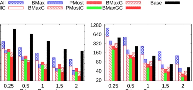
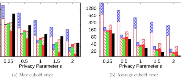
6.2.1 Varying Privacy Parameter ² . . . 81
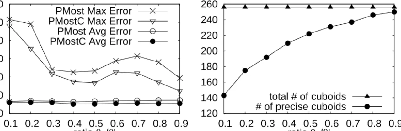
6.2.2 Varying Variance Threshold θ0 . . . 83
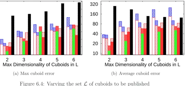
6.2.3 Varying Set of Cuboids to be Published . . . 84
6.2.4 Noise in Different Cuboids . . . 85
6.2.5 Scalability: Number and Cardinality of Dimensions . . . 85
6.2.6 Efficiency of Different Publishing Algorithms . . . 88
6.2.7 Background Knowledge v.s. Noise . . . 89
6.3 Summary . . . 90
Chapter 7 Conclusions and Future Work . . . 92
7.1 Conclusions . . . 92
7.2 Future Work . . . 93
List of Figures
1.1 Fact Table and a count data cube . . . 3
1.2 Advantage of using privacy-preserving data cubes for data analytics . . . 4
2.1 Lattice of cuboids in a data cube . . . 11
3.1 Lattice of cuboids and variance magnification of noise . . . 26
5.1 A shortest sequence of moves for 2×2×2 case . . . 74
6.1 Varying privacy parameter ² in the Adult dataset . . . 81
6.2 Varying privacy parameter ² in the Nursery dataset . . . 82
6.3 Varying θ0 in Algorithm 2 (for PMost and PMostC) . . . 83
6.4 Varying the set L of cuboids to be published . . . 84
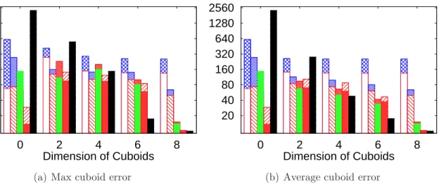
6.5 Max cuboid error as dimensionality varies, when all cuboids are released . . 85
6.6 Varying dimensionality of fact table (cardinality equals to 7) . . . 86
6.7 Varying cardinality of dimensions (7 dimensions) . . . 86
6.8 Differentially private data cube publishing time (in seconds) . . . 87
6.9 Efficiency of different algorithms (subroutines of publishing algorithms) . . . 87
Chapter 1
Introduction
Data cubes play an essential role in multidimensional data analysis and fast OLAP queries. Simply put, adata cube of afact table (i.e. a multidimensional table) consists of a collection of cuboids, where each cuboid is generated by grouping records in the table by a subset of dimensions. The publishing of data cubes can facilitate and speed up all kinds of data mining algorithms. However, as the underlying data often is sensitive, publishing all or part of a data cube may endanger the privacy of individuals. For example, privacy concerns prevent Singapore’s Ministry of Health (MOH) from performing wide-scale monitoring for adverse drug reactions among Singapore’s three main ethnic groups, none of which are typically included in pharmaceutical companies’ drug trials. Privacy concerns also limit MOH’s published health summary tables to extremely coarse categories, reducing their utility for policy planning. Institutional Review Board (IRB) approval is now required for access to most high-level summary tables from studies funded by the US National Institutes of Health, making it very hard to leverage results from past studies to plan new studies. In these, and many other scenarios, society can greatly benefit from the publication of detailed and high-utility data cubes that also preserve individuals’ privacy. This thesis studies several interweaving fundamental problems of data privacy in data cubes, including how to publish a data cube in such a way that it can be browsed by users and utilized by different data mining algorithms without endangering individuals’ privacy, how to improve the data quality in such privacy-preserving data cubes, and how to guarantee individuals’ privacy information even if adversaries have part of the data cube in their background knowledge.
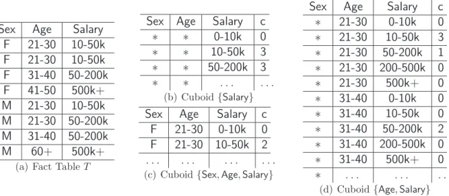
The data cube of a fact table consists of cells and cuboids. A cell aggregates the rows in the fact table that match on certain dimensions. For example, consider the fact table in Figure 1.1(a) with three dimensions, to be aggregated with count measure c. As in Figures 1.1(b)-1.1(d), a cuboid can be viewed as the projection of a fact table on a subset of dimensions, producing a set of cells with associated aggregate measures.
We aim to preserve data privacy so that individual level properties of the data are not disclosed to adversaries. The definition of privacy has needed to become stronger, partly because abundant data is now available from more and more sources on the Internet (ad-versaries have morebackground knowledge), and computers become more and more powerful (adversaries have strongercomputational power). For example, according to the definition of privacy (or security) proposed in 1980s [13, 17], individuals’ data is said to be secure if it can-not be computed from a linear combination of rows in the released table. However, because of the above two reasons, such protection of data privacy is far from sufficient nowadays, as shown in the following examples in data cubes.
With background knowledge, an adversary can easily infer sensitive information about an individual from a published data cube [33, 42, 78]. For example, in the data cube in Figure 1.1, if we know that Alice is aged 31-40 and is in the table, the count measure c in cuboid {Age,Salary} tells us her salary is 50-200k. If we know Bob is in the table and is aged 21-30, we learn there is a 75% chance that his salary is 10-50k and a 25% chance it is
50-200k. If we also know that Carl, aged21-30 and with salary50-200k, is in the table, then the values of countin cuboid {Age,Salary} tell us Bob’s salary is 10-50k.
Even publishing large actual aggregate counts is still not safe, if an adversary has enough background knowledge. For example, suppose there are 100 individuals in a fact table (Sex,Age,Salary), and we publish two cells (∗, ∗, 10-50k) and (∗, ∗, 50-200k), both with count equal to 50. Suppose the adversary knows everyone’s salary except Bob’s: if 49 people have salary 10-50k and 50 have 50-200k, it can be inferred that Bob’s salary is 10-50k.
Sex Age Salary F 21-30 10-50k F 21-30 10-50k F 31-40 50-200k F 41-50 500k+ M 21-30 10-50k M 21-30 50-200k M 31-40 50-200k M 60+ 500k+
(a) Fact TableT
Sex Age Salary c
∗ ∗ 0-10k 0
∗ ∗ 10-50k 3
∗ ∗ 50-200k 3
∗ ∗ . . . . (b) Cuboid{Salary}
Sex Age Salary c F 21-30 0-10k 0 F 21-30 10-50k 2 . . . . (c) Cuboid{Sex,Age,Salary}
Sex Age Salary c
∗ 21-30 0-10k 0 ∗ 21-30 10-50k 3 ∗ 21-30 50-200k 1 ∗ 21-30 200-500k 0 ∗ 21-30 500k+ 0 ∗ 31-40 0-10k 0 ∗ 31-40 10-50k 0 ∗ 31-40 50-200k 2 ∗ 31-40 200-500k 0 ∗ 31-40 500k+ 0 ∗ . . . . (d) Cuboid{Age,Salary}
Figure 1.1: Fact Table and a count data cube
We apply the notion of ²-differential privacy [21] in data cube publishing. Compared to previous techniques for privacy-preserving data publishing (see [1, 32] for surveys), dif-ferential privacy makes very conservative assumptions about the adversary’s background knowledge and computational power. It guarantees privacy against adversaries with arbi-trary amounts of knowledge about each individual, as long as the data of individuals are independent of each other [44]. In particular, mechanisms satisfying this definition guarantee privacy against adversaries who may know every row in the database except one.
Informally, differential privacy guarantees that the presence/absence or specific value of any particular individual’s record has little effect on the likelihood that a particular result is returned to a query. Thus an adversary cannot make meaningful inferences about any one individual’s record values, or even whether the record was present.
One way to achieve differential privacy is to add random noise to query results, called the Laplacian mechanism [21]. In this mechanism, the noise is carefully calibrated to the query’ssensitivity, which measures the total change of the query output when one individual record/tuple is deleted or added in the database. For example, if the query is to count how many rows satisfying property P, its sensitivity is one, because deleting/adding one row
%& ' ( ) %& &' * + , - & !" #$ %& '( )%&&' * . / 0 1 21 3 456 // %& ' ( ) %& &' * &7 % & !" #$
(a) Privacy-preserving data mining algorithms
!" # $ % !" "# & '" ( ) " * " ++ !" #$ %!""# & ) $ , - . / 0 10 2 345 .. "6 ! " ++ 789: ;< =>?@@ ; A A8A BC D; A:?A E
(b) Privacy-preserving data cube
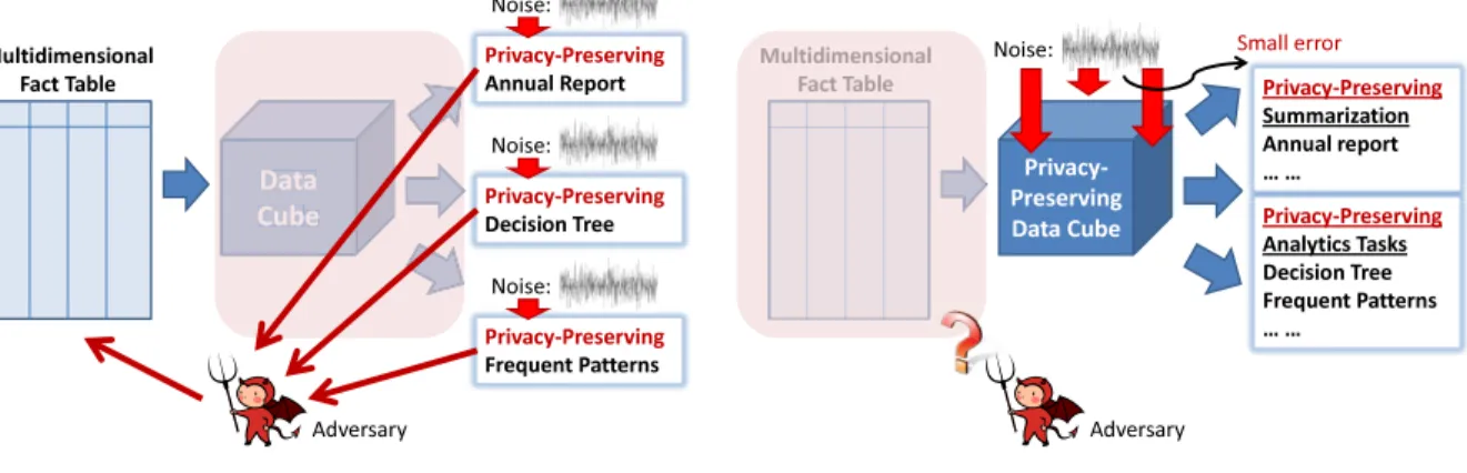
Figure 1.2: Advantage of using privacy-preserving data cubes for data analytics changes the count by at most one. As the variance of the noise increases, the privacy guarantee becomes stronger, but the utility of the result drops. Another way is exponential mechanism, where different outcomes are sampled according to noisy scoring functions [62]. There is a line of works which directly apply the notion of differential privacy in data mining algorithms (e.g. constructing decision trees [31] and mining frequent patterns [8]). The deficiency of such works is depicted in Figure 1.2(a): A data analyst may run different data mining algorithms on the same table. Although each data mining algorithm is claimed to be privacy-preserving independently, the adversary can combine results from different algorithms to enhance their background knowledge about the fact table. Such background knowledge reveals correlation inside the fact table, and thus could be more dangerous and make individuals’ privacy more vulnerable. For example, each algorithm reports the number of rows satisfying property P in its output, with a sample drawn from some noise distribu-tion inserted into this number to preserve privacy; each algorithm is privacy-preserving by itself; however, if the adversary averages the answers from multiple algorithms, the expected squared error can be reduced significantly, with individuals’ privacy endangered.
Our proposal is depicted in Figure 1.2(b). We first publish a data cube in a privacy-preserving way. This data cube can be reused by infinite number of data mining or processing
algorithms. As long as these algorithms do not access the real fact table, the same privacy guarantee is preserved from the data cube to these algorithms. The adversary cannot benefit from combining results from different algorithms (Theorems 2.1.3 and 5.2.5). So the first question is: how to improve the data quality in privacy-preserving data cubes.
To publish an ²–differentially private data cube over d dimensions, there are two natural methods. (i) We can compute the count measure from the fact table, and then add noise to each cell in each cuboid. There are 2d cuboids and modifying the value of one individual’s
record could change the count of some cell in every cuboid by 1. So the sensitivity (total change) is 2d, and according to [26], each cell needs Laplace noise Lap(2d/²)1. This results in noise with zero mean and variance equal to 2·4d/²2 added to every count. For reasonable values of d, the variance is too large, which destroys the utility of the data cube. The same idea is applied in one of the two approaches proposed in [5] to publish a set of marginals of a contingency table. (ii) Or, we can directly add noise to the fact table, or the base cuboid ({Sex, Age, Salary} in Figure 1.1(c)). Then Lap(1/²) suffices. We compute the other cuboids from the noisy base cuboid to ensure differential privacy. However, noise in high-level cuboids, such as {Salary}, will be magnified significantly, and thus the utility will be low. For example, if a cell in a high-level cuboid aggregates N cells in the base cuboid, the variance of noise in that cell is magnified by N times as well. This idea can be applied to universal histograms, but noise accumulation also makes them ineffective there [40]. Another possible way is to treat each cell as a query, and apply methods in [51] to answer a workload of count queries while ensuring differential privacy. But this approach is not practical in our context, as its running time/space is at least quadratic in the number of cells.
If we browse measures across differentially private cuboids, the sums may not match the totals recorded in other higher-level cuboids, because independent noise is inserted into different cells. According to a Microsoft user study [47], users are likely to accept these kinds
of small inconsistencies if they trust the original data and understand why the inconsistencies are present. However, if the users do not trust the original data, they may interpret the inconsistencies as evidence of bad data. So it is desirable to enforce a requirement for correct roll-up totals across dimensions in the cuboids to be published. Consistency also boosts accuracy of differentially private data publishing in some cases, e.g., in answering one-dimensional range queries [40]. The second question is: how to enforce consistency in differentially private data cubes while retaining or even improving the data quality.
Some cuboids within a data cube, especially the high-level ones, may be published exactly to both users and adversaries, either (i) because they are background knowledge that can be easily obtained (for example, how many males or females in a company) or (ii) it is required according to policies or requirement of data users. Such exact partial information or background knowledge about a data cube can cause privacy breaches when combined with differential privacy [43]. Intuitively, the more exact information released from a data cube, the more noise needed to be inserted into the rest part to preserve the same level of privacy. The third question is: how to calibrate noise in data cubes subject to certain exact background knowledge while we are trying to improve the data quality.
Contributions. Towards answering the above three questions about publishing privacy-preserving data cubes, the studies in this thesis can be summarized as follows.
• We study how to publish all or part of a data cube for a given fact table, while ensuring²-differential privacy and limiting the variance of the noise added to the cube. We propose a general noise control framework in which a subset Lpre of cuboids is
computed from the fact table, plus random noise. The remaining cuboids are computed directly from those inLpre, which is the “source of noise”. When Lpre is larger, each of
its members requires more noise, but the cuboids computed fromLpre accumulate less
noise. So a clever selection of Lpre can reduce the overall noise. This framework can
Lpre. With a larger search space, the generalized framework may potentially improve
the precision in a data cube while preserving the same level of privacy, which will be demonstrated both in theory and in experiments later in this thesis.
• We consider several publishing scenarios that fit the needs of data agents, e.g., the Ministry of Health. In the first scenario, a set of cuboids are identified to be released, and the goal is to minimize the max noise in the cuboids. In the second scenario, MOH has a large body of cross-tabulations that can be useful for urban planners and the medical community. A weighting function indicates the importance of releasing each cuboid. The question is, which of these cuboids can be released in a differentially private manner, while respecting a given noise variance bound for each cell (called precise cuboids)–the goal is to maximize the sum of the weights of the released precise cuboids. In the third scenario, a threshold of noise variance is specified for each cuboid to be released. The goal is to minimize the max relative ratio between the noise variance and the expected threshold in each released cuboid.
We formalize these scenarios as three optimization problems for the selection of Lpre,
as well as the amount of noise in each cuboid of Lpre in the generalized framework,
prove that they are NP-hard, and give efficient algorithms with provable approximation guarantees. For the first problem or the third, the max noise variance or the max relative ratio, respectively, in published cuboids will be within a factor (ln|L|+ 1)2 of optimal, where |L| is the number of cuboids to be published; and for the second, the number/weight of precise cuboids will be within a factor (1−1/e) of optimal.
• We show how to enforce consistency over a differentially private data cube by com-puting a consistent measure from the noisy measure released by a differentially private algorithm. We minimize theLp distance between the consistent measure and the noisy
the fact table when enforcing consistency. TheLp distance from the consistent measure
to the real measure is at most doubled compared with the distance from the inconsis-tent measure to the real measure, for general p. The consistency-enforcing techniques in [5] are similar to our L∞ version. But we show that the L1 version yields a much better theoretical bound on error than the L∞ version. More surprisingly, we show
that in the L2 version, the consistent measure provides even better utility than the original inconsistent noisy measure, based on the theory of (weighted) least squares and the best linear unbiased estimator (BLUE). We provide efficient algorithms to compute such consistent measures (minimizeL2 distance), with running time linear in the number of cells, while previous techniques have at least quadratic running time.
• We study the relationship between the amount of background knowledge an adversary has and the amount of noise needed to be injected in the scenario of data cubes. We consider some cuboids that have to be released exactly as the background knowledge. We generalize results in [43] about using generic differential privacy to handle such background knowledge. Based these studies, we show how to plug generic differential privacy into our noise control frameworks to limit the variance of the noise added to data cubes subject to background knowledge in forms of exact cuboids.
• All of our techniques proposed in this thesis are both proved to be sound in theory and evaluated with real datasets to verify their effectiveness in practice.
Organization. Chapter 2 provides background for data cubes and differential privacy, together a review of related work. Chapter 3 introduces our noise control publishing frame-works, and different optimization algorithms aiming at different objectives. Chapter 4 shows how to enforce consistency across cuboids based on differentLp distances and analyzes their
properties. Chapter 5 studies how to handle adversary’s background knowledge. All experi-ments are reported in Chapter 6. Chapter 7 gives conclusion and future directions.
Chapter 2
Background and Related Work
We present background materials and related work of this thesis in this chapter. We start with a formal definition ofdifferential privacy[26, 20] and its application indata cubesin Sec-tion 2.1. We then introduce some related work in SecSec-tion 2.2, including relevant techniques to apply this notation of privacy in privacy-preserving data publication (Section 2.2.1) and data mining (Section 2.2.2), and some recent progress on extending the notation of differential privacy for more general context or with weaker/stronger privacy guarantee (Section 2.2.3).
2.1
Background and Notations
The notion of differential privacy was originally introduced in [20, 26]. It is general enough to handle data models including unstructured data like search logs and structured data like histograms and graphs, as long as they can be represented as a vector of entries. In this thesis, we focus on data cubes, a modeling and analytical tool for multidimensional data. We will introduce basic concepts of data cubes and differential privacy in this section.
2.1.1
Data Cubes
Afact tableT is a multidimensional table withdnominal dimensionsA={A1, A2, . . . , Ad}.
We use Ai to denote both the ith nominal dimension and the set of all possible values for
this dimension. Let |Ai|denote the number of distinct values (i.e., cardinality) of dimension
The data cube[36] of a fact tableT can be considered as the projections ofT onto subset of dimensions. A data cube consists of cells and cuboids. More formally, a cell a takes the form (a[1], a[2], . . . , a[d]), where a[i] ∈ (Ai∪ {∗}) denotes the ith dimension’s value for this
cell, and it is associated with certain aggregate measure of interest. In this thesis, we first focus on thecount measure c and discuss how to handle other measures like the summation measure sum(sum of values associated with all rows in a cell) and the average measure avg
(average of values associated with all rows in a cell) in Section 3.4.2. The count measure
c(a) is the number of rows r in T that are aggregated in cell a (with the same values on non-∗ dimensions of a). Formally, let c(a) = |{r∈T | ∀1≤i≤d, r[i] =a[i]∨a[i] =∗}|.
A cell a is an m-dim cell if values of exactly m dimensions a[i1], . . . , a[im] are not ∗. An
m-dim cuboid C is specified by m dimensions [C] = {Ai1, . . . , Aim}, and it consists of all m-dim cells a such that ∀1≤ k ≤m, a[ik]∈ Aik, and a[j] = ∗ for all j /∈ {i1, . . . , im}. We use C and [C] interchangeably to denote either a cuboid or the set of dimensions specifying this cuboid. A cuboid C can be interpreted as the projection of T on the set of dimensions [C]. Thed-dim cuboid is called thebase cuboid and the cells in it are base cells.
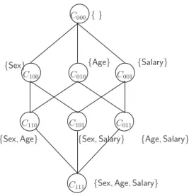
For two cuboids C1 and C2, if [C1] ⊆ [C2] (denoted as C1 ¹ C2), then for a large class of measures, such ascount c, summation sum, and averageavg, cells in C1 can be computed from C2 [36]. The cuboid C1 is said to be an ancestor of C2, and C2 is a descendant of C1. LetLall denote the set of all cuboids. Clearly, (Lall,¹) forms a lattice.
Example 2.1.1 Fact table T in Table 1.1 has three dimensions: Sex = {M, F}; Age = {
0-10,11-20, 21-30, 31-40, 41-50,51-60, 60+}; andSalary ={0-10k, 10-50k, 50-200k, 200-500k,
500k+}. Figure 2.1 shows the lattice of cuboids of T. Cuboid {Age,Salary} can be computed from T. For example, to compute the cell (∗, 21-30, 10-50k), we refer to the table T for rows (M, 21-30, 10-50k) and (F, 21-30, 10-50k), and we find three such rows. As{Salary} ⊆ {Age,Salary}, cuboid {Salary} can be computed from cuboid {Age, Salary}. For example, to compute cell (∗, ∗, 10-50k), we aggregate cells (∗, 0-10, 10-50k), . . . , (∗, 60+, 10-50k).
C110 C101 C011
C111
C100 C010 C001
C000
{Sex,Age,Salary} {Sex,Age} {Sex,Salary} {Age,Salary}
{Age} {Salary} { }
{Sex}
Figure 2.1: Lattice of cuboids in a data cube
2.1.2
Differential Privacy
Differential privacy (DP for short in the rest of this thesis) is based on indistinguishability between pairs of neighboring tables. Two tablesT1 and T2 are neighborsif they differ by one row, i.e., inserting or deleting one row from T1 yields T2. Formally, let T be the set of all possible table instances with dimensions A1, A2, . . . , Ad, and Γ(T) ={T0 | |(T −T0)∪(T0−
T)|= 1} ⊆ T the set of all neighbors of T. Clearly, T1 ∈Γ(T2) implies T2 ∈Γ(T1).
Definition 2.1.1 (Differential privacy [21]) A randomized algorithmKis²-differentially
private if for any two neighboring tables T1 and T2 and any subset S of the output of K,
Pr [K(T1)∈S]≤exp(²)×Pr [K(T2)∈S],
where the probability is taken over the randomness of K and ² is a fixed value.
Consider an individual’s concern about the privacy of her/his record r. When the pub-lisher specifies a small ², Definition 2.1.1 ensures that the inclusion or exclusion of r in the fact table makes little difference in the chances ofK returning any particular answer.
Some papers use a slightly different definition of neighbors: T1 and T2 are neighbors if they have the same cardinality and T1 can be obtained from T2 by replacing one row (²-indistinguishable [26]). Our algorithms and techniques in this thesis also work with this definition, if we double the noise, because it has been shown that any mechanism satisfies ²-indistinguishability if and only if it satisfies 2²-differential privacy.
Tools to Achieve Differential Privacy
There are two popular ways to achieve ²-differential privacy, the Laplacian mechanism [21] and the exponential mechanism [62]. In most (but not all) cases, the Laplacian mechanism is used for data publication, whereas the exponential mechanism is used for optimization problems. And, the Laplace mechanism is a special case of the exponential mechanism.
Throughout this thesis, we useR to denote the set of all real numbers. LetF :T → Rn
be a function that produces a vector of length n from a table instance. In our context (data cubes), F computes the set of cuboids to be released. In the Laplacian mechanism, for a table T, a noisy version ˜F(T) of F(T) is released to preserve differential privacy, and the amount of noise is carefully calibrated according to the sensitivity of F.
Definition 2.1.2 (Sensitivity [21]) The L1 global sensitivity of F is:
S(F) = max T2∈T µ max T1∈Γ(T2)kF(T1)−F(T2)k1 ¶ , where kx −yk1 = P
1≤i≤n|xi − yi| is the L1 distance between two n-dimensional vectors
x=hx1, x2, . . . , xni and y=hy1, y2, . . . , yni.
For example, if the function F is to count how many rows satisfying property P, then S(F) = 1, because deleting/adding one row in T changes the count F(T) by at most one.
Definition 2.1.3 (Laplacian distribution) Let Lap(λ) denote a sample Y taken from a zero-mean Laplace distribution with probability density function h(x) = 1
2λ exp(−|x|/λ). We
have Pr [|Y| ≥z] = exp(−z/λ), E [Y] = 0, and variance Var [Y] = 2λ2. We write hLap(λ)in
to denote a vector of n independent random samples hY1, Y2, . . . , Yni, where Yi ∼Lap(λ).
The following theorem quantifies how much noise to be injected into F(T) is sufficient.
Theorem 2.1.1 (Laplacian mechanism [26]) Let F : T → Rn be a query sequence of
length n against a table T ∈ T. The randomized algorithm that takes as input table T and output F˜(T) = F(T) + hLap(S(F)/²)in is²-differentially private.
In the exponential mechanism, for a given table T ∈ T, an outcome r from a domain O is randomly selected according to some scoring function s:T × O → Rand a base measure µ : O → R. s and µ are public knowledge for everyone including adversaries. To achieve differential privacy, the distribution for selecting (and publishing) r is carefully calibrated with the scoring function s and the base measure µ, as in the next theorem.
Theorem 2.1.2 (Exponential mechanism [62]) For an input table T ∈ T, the
probabil-ity of selecting an outcome r ∈ O, is proportional to exp(²·s(T, r))·µ(r). In particular,
the density function f(r) = R exp(²·s(T, r))·µ(r)
r0exp(²·s(T, r0))·µ(r0)
.
Then selecting and publishing r satisfies ²∆(s)-differential privacy, where
∆(s) = max
r∈O maxT2∈T T1max∈Γ(T2)|s(T1, r)−s(T2, r)|.
Suppose the quality of outcomes is measured by the scoring function s. Based on the above theorem, [62] shows that, using the exponential mechanism, there are some guarantees on the outcome’s quality while the ²-differential privacy is preserved.
The transition and composition properties of differential privacy are frequently used in our and others’ research on differentially private algorithms. These two properties allow the combining of the publications or outcomes of several differentially private algorithms.
Theorem 2.1.3 (Transition and composition properties [62, 59]) LetKi(·)orKi(·,·)
be a randomized algorithm which is ²i-differentially private. Then,
1. For a table T, outputting K1(T) and K2(T,K1(T)) is (²1+²2)-differentially private.
2. For any input table T and any algorithm K, outputting K1(T) and K(K1(T)) is ²1 -differentially private.
3. For any two input tablesT1 andT2 such that T1∩T2 =∅, outputtingK1(T1)andK1(T2) is ²1-differentially private.
2.2
Related Work
Since ²-differential privacy (DP) [26] was introduced, many techniques have been proposed for different data publishing and analysis tasks (refer to [21, 22, 24, 84] for a comprehensive review). We will mainly review three aspects of recent research on developing (differential) privacy-preserved algorithms: the first aspect is about data publishing and query answering algorithms (Section 2.2.1); the second is about data mining algorithms (Section 2.2.2); and the third is extensions to the notion of differential privacy (Section 2.2.3).
2.2.1
Differentially Private Data Publishing
Differential privacy has been applied in various data management and processing systems [3, 4, 11, 59, 81]. In this part, we focus on (differentially) private histograms, count queries, multidimensional data publishing, and batch-query processing techniques, as data cubes are
essentially multidimensional count queries in nature, and cuboids to be published can be thought as a batch of queries against the fact table to be answered.
Other mechanism to achieve differential privacy
Some functionsF, e.g.., the median of a set of numbers, may have very large sensitivityS(F), e.g., the range of the universe. So the resulting Laplacian mechanism may need to inject too much noise. To achieve differential privacy for a fixed table T, the amount of noise needed to be injected is actually proportional to the local sensitivity S(F, T) = maxT0∈Γ(T)kF(T)−
F(T0)k
1 [66]. However, it may already violate the differential privacy to calibrate noise to S(F, T). So it is proposed in [66] to first obtain an approximate upper bound of S(F, T) (called smooth sensitivity) without violating differential privacy, and then calibrate noise to this upper bound. The resulting privacy guarantee, (², δ)-differential privacy [25], is weaker than ²-differential privacy by additive factor δ. Also note that a more direct way to achieve (², δ)-differential privacy is to addGaussian noiseintoF(T) [25], and the techniques proposed in this thesis can be also extended for (², δ)-differential privacy.
For a single counting query, a method to ensure differential privacy (geometric mecha-nisms) [26] has been shown to be optimal under a certain user utility model [34], and the Laplacian mechanism [26] is proved to be nearly optimal.
Recently, Li et al. [56] proposes the compressive mechanism based on compression tech-nique. The basic idea is to insert noise into the compact synopsis, which is constructed using random projections and has potentially smaller sensitivity than the original table.
Noise complexity of mechanisms for answering linear queries
Hardt and Talwar [39] study the noise complexity of differentially private mechanisms in the setting where the user asks a set of linear queries non-adaptively. The noise complexity means how much noise is necessary and sufficient to make the query answers differentially
private. They show that the noise complexity is determined by two geometric parameters associated with the set of queries, and derive nearly matching upper and lower bounds of the amounts of noise needed to make the answer differentially private. This line of research is followed by [38] and [37] to obtain better asymptotic bounds.
Both a one-dimensional histogram and a multidimensional data cube can be considered as sets of linear queries. So the above upper and lower bounds also apply when we want to publish them. But it is possible to utilize the special structure of such queries in histograms or data cubes to further reduce the amount of noise needed. Also, instead of deriving asymptotic bounds of noise, there is a line of research on how to model the amount of noise needed as an objective function and solve an optimization problem to reduce noise in answering batches of linear queries. Those different lines of research will be introduced in the following parts. And it is an interesting and still quite open problem to compare different lines of methods using systematical and comprehensive experiments.
One-dimensional histogram
Histogram can be thought as a one-dimensional data aggregation and is an important tool for answering range queries. Hay et al. [40] propose an approach based on a hierarchy of intervals, so-called universal histogram. Noise is injected into answers to count queries on these intervals, and these noisy interval can be used to answer all possible range queries. A naive method injects noise directly into the data domain, and answers range queries by aggregating noisy data in the original domain. The error in the answers, if measured by variance of noise, is reduced from O(m/²2) in the naive method to O(log3m/²2) in the approach of [40]. Xiao et al. [80] propose to use the Haar wavelet for range count queries with similar error bound guarantee, which can also handle multidimensional data.
The hierarchy structure in [40] is essentially a balanced binary tree similar to interval tree [14]. A natural idea to reduce error could be optimize this tree structure, for example,
by varying the depth or fanout of the tree. However, to guide such optimization, we may need to access the statistics of the origin data, which already violates our privacy guarantee. There are mainly two differentially private ways to do such optimization: the first one is to use exponential mechanism, assigning a score for each possible structure, and selecting the (approximately) best one using randomized algorithms; and the second one borrows the ideas from smooth local sensitivity [66], using a noisy version of the statistics from we need to guide the optimization – accessing such noisy statistics is differentially private, and it is accurate enough for the purpose of optimization. These ideas are used in [67, 82, 83] to reduce error in (multidimensional) histograms for count queries, and used in [79] to optimize parameters in noise injection for reducing relative error. Such differentially private data publication techniques are data-dependent. Other techniques that do not rely on statistics about the input database are data-independent [84], including [40, 80] and ours.
Multidimensional data aggregation
Some techniques designed for differentially private histogram publication can be extended for multidimensional data aggregation and publication (e.g. [80], [82], and [67]). For example, Xiao et al. [80] also extend their wavelet approach to nominal attributes and multidimen-sional count queries. Some other differentially private techniques are designed particularly for publishing multidimensional data, e.g., [15] and [5] which are introduced below.
Cormodeet al. [15] consider how to answer multidimensional range queries in a differen-tially private way. They propose to use a quad-tree structure with Laplacian noise inserted first, and then answer range queries using the noisy quad tree.
Barak et al. [5] show how to publish a set of marginals of a contingency table while ensuring differential privacy. Here, marginals of a contingency table are essentially cuboids in our data-cube language. One of their two approaches adds noise to all the cuboids to be published. Since noise is injected into different cuboids independently, there is inconsistency
across different noisy cuboids. [5] proposes a method based on linear programming (LP) and rounding, which computes a consistent data cube from the noisy inconsistent one and minimizes theirL∞distance. At the same time, integrality can be also enforced and negative
numbers can be removed in the publishing. In the later part of this thesis, we will show that minimizing the L1 distance yields a much better theoretical bound on error. The other approach in [5] is similar, but moves to the Fourier domain at first, and add noise to Fourier coefficients. The major reason for moving to the Fourier domain is that the Fourier coefficients are the “sufficient statistics” for marginals of a contingency table, in the sense that if any Fourier coefficient is ignored, there is a free degree of freedom which can lead to unbounded error between true and reported values [60]. But unlike our work, they do not optimize the publishing strategy (the same amount of noise is injected into all cuboids or all Fourier coefficients). Moreover, the number of variables in the linear programming equals the number of cells (often > 106 in our experiments). So LP-based methods are mainly of theoretical interests and can only handle data cubes with small numbers of cells.
Optimizing noise for batches of linear queries
Linear count queries ask questions like “how many rows in the table satisfying property P.” When the database is modeled as a frequency vector, a linear count query can be presented as a vector (specifying the property P). Suppose there is a batch of linear count queries to be answered, which is presented as a query matrix(with query vectors as its columns), the very basic method is to insert noise into the frequency vector and then compute the multiplication of the noisy frequency vector and the query matrix. There is a line of work [51, 52, 53, 85] on how to reduce error in answers to the given batch of linear queries.
Liet al. [51] propose a general framework calledmatrix mechanismto support answering a given workload of count queries while preserving differential privacy. The basic idea is to choose an alternative set of queries, represented as a strategy matrix, answer these strategy
queries first using the Laplacian mechanism, and compute each query in the input workload using the noisy answers to the strategy queries. The strategy matrix is carefully selected so that every input query can be answered and the total error (sum-square error) is minimized. They [52] propose an efficient algorithm to select a near-optimal strategy matrix, and also give a lower bound of the total error one can get using the matrix mechanism [53]. While [80] and [40] can be unified in the framework of matrix mechanism, the specific algorithms given in [40, 80] are more efficient than the matrix multiplication used in [51, 52].
Yuanet al. [85] introduce a variant of the matrix mechanism, calledlow-rank mechanism. They propose practical differentially private technique for answering batch queries with high accuracy, based on a low rank approximation of the query matrix. They prove that the accu-racy (measured by sum-square error) provided by their techniques is close to the theoretical lower bound for any mechanism to answer a batch of queries under differential privacy. Note that [52] and [85], aiming at the same goal, are developed independently and to be published in the same year, so it will be very interesting to compare their performance.
Cormodeet al. [16] apply the matrix mechanism to publish data cubes. A data cube can be modeled as a batch of linear queries, each of which corresponds to a cube cell. But as the number of cells is huge, the original matrix mechanism is inapplicable as the matrices involved are too huge to be manipulated. [16] proposes an efficient noise-optimization algorithm and a consistency-enforcing algorithm via grouping matrix entries that correspond to cells in the same cuboid. So the matrices involved become small enough to be handled. Another approach proposed in [16] tries to optimize the amounts of noise to be injected into Fourier coefficients of cube cells, so that the overall noise is minimize. Different from our work, they use sum-square error to measure the overall noise, while we use max-square error.
Comparison to other privacy notations
Agrawal et al. [2] study how to support OLAP queries (cells or cuboids in data cubes) while ensuring a limited form of (ρ1, ρ2)-privacy, by randomizing each entry in the fact table with a constant probability. An OLAP query on the fact table can be answered from the perturbed table within roughly p|dataset| [5]. (ρ1, ρ2)-privacy is in general not as strong as ²-differential privacy. Also, the error incurred by this method [2] depends on the dataset size; in our framework, the amount of noise to be added is data-independent, only determined by the number of cuboids to be published and the structure of the fact table.
In data publication, differential privacy provides much stronger privacy guarantees than other privacy concepts based on deterministic algorithms do, such ask-anonymity [69, 70, 73, 72], and its extensionl-diversity [57] andt-closeness [54]. These privacy-preserving notations and techniques suppress or generalize entries in the table such that groups of tuples appear indistinguishable or uninformative about sensitive attributes. However, these techniques are vulnerable if the adversary has enough background knowledge. [74, 75, 76] study how to specify authorization and control inferences for OLAP queries in the data cube. They aim to detect OLAP queries with either unauthorized accesses or malicious inferences.
2.2.2
Differentially Private Data Mining
Data mining algorithms usually access sensitive information about individuals, such as med-ical records and search logs. It is an urgent task to develop privacy-preserving techniques so that data owners are willing to share data miners with more data. For example, the notation of differential privacy has been applied to releasing query and click histograms from search logs [35, 45], recommender systems [61], publishing commuting patterns [58], publishing re-sults of machine learning [9, 12, 41, 86], clustering [30, 66], decision tree [31, 64], mining frequent patterns [8], and aggregating distributed time-series [68].
There are two basic ideas to preserve differential privacy in data mining algorithms, based on the Laplacian mechanism and the exponential mechanism, respectively. Using the Laplacian mechanism, data mining algorithms take Laplacian-noise-injected data as the input. Because of the transition and composition property (Lemma 2.1.3), the same level of differential privacy is preserved in the data mining results as in the noisy data. In another way, the exponential mechanism is applied internally in data mining algorithms. When the algorithm needs to branch, it randomizes the branch selection according to some utility function. For example, in decision tree learning, each branch determines which attribute to be split and the utility function could be information gain of splitting an attribute.
2.2.3
Extension of Differential Privacy
We now introduce some variants of differential privacy, which can be applied for more general context, and may have weaker or stronger privacy guarantee. They may also have different assumptions about the adversary’s background knowledge (prior belief on the data).
The first one is (², δ)-differential privacy [25], which was already mentioned in Sec-tion 2.1.2. It is a weaker variant of ²-differential privacy, and the difference is that, in the definition of ²-differential privacy (Definition 2.1.1), the inequality is replaced with Pr [K(T1)∈S] ≤ exp(²)×Pr [K(T2)∈S] +δ. (², δ)-differential privacy trades off privacy for utility, via either smoothing local sensitivity or injecting Gaussian noise.
Generic differential privacy proposed in [43] takes background knowledge of adversaries into consideration. It tries to fix bugs in the assumption of differential privacy, by modeling the neighbors as two closest tables (or databases) that are consistent with the background knowledge. Intuitively, the more knowledgeable the adversary is, the more noise needs to be injected, and this notation quantifies how much noise is necessary. It provides us some hints on how to select the mysterious parameter ². We will apply this notation in Chapter 5 of this thesis, and thus more details about this notation will be introduced there.
Pan-privacy [29] provides a stronger guarantee that the pan-private algorithms retain the privacy properties even if their internal state becomes visible to adversaries. The study of this notation was initiated in algorithms for data streams [23, 29, 63], as when sketches used in streaming algorithms are hacked by adversaries, previous privacy guarantees will be easily broken. Also event-level pan-privacy and user-level pan-privacy are distinguished in [28]. Also because real system is usually required to continually generate outputs, the study of (pan-)differential privacy under continual observation is initiated in [28].
Pufferfish [44] is a framework to create new privacy notations that are customized to given applications. The Pufferfish framework provides differential privacy-like probabilis-tic guarantee but with more expressive power in a general context. It allows expertise to specify: i) what secrets about individual users need to be protected, which are expressed as a potential set of secrets and pairs of secrets needed to be discriminated from each other; and ii) adversaries’ belief in how the data were generated and their knowledge about the database. In particular, ii) is specified because as discussed in [27, 43], proper assumption about knowledge of adversary may improve the utility of privacy guarantees. Previous dif-ferential privacy can be analyzed within the Pufferfish framework, and this framework also enjoys useful (and more general) properties, like composition and self-composition.
Differential identifiability [48] is proposed recently to give more quantitative guidelines on how to select the value of ² based on the level of privacy required. It also has implicit assumptions and models about how the data is generated in adversary’s belief.
Chapter 3
Optimizing Noise Sources in Data
Cubes
Problem Description
Given a d-dimensional fact table T, we aim to publish a subset L of all cuboids Lall with
measure ˜c(·), a noisy version of thecount measurec(·) inL, using an algorithmKthat ensures ²-differential privacy. In particular, for any cellain a cuboid inL, we want to publish anoisy count measure ˜c(a) using the differentially private algorithm K. With the level of privacy fixed (i.e. the parameter ² in differential privacy is fixed), we want to minimize the error in ˜
c(·), or the difference betweenc(·) and ˜c(·), so that the utility of data is preserved as well. In this chapter, we will first discuss how to measure the error in publishing algorithms and possible objectives in Section 3.1, and then introduce noise-control publishing algorithms that (approximately) achieve these objectives in Section 3.2 and Section 3.3.
3.1
Measuring Noise and Publishing Objectives
We measure the utility of an algorithm by the variance of the noisy measure it publishes. As we apply the Laplacian mechanism in Theorem 2.1.1, we will show noisy measure ˜c(·) published by our algorithms is unbiased, i.e., the expectation E [˜c(a)] = c(a). So for one cell, the noise varianceVar [˜c(a)] is equal to themean squared error of the noisy measure ˜c(a) we publish, and we use it to measure the noise/error in ˜c(a) for one cella:
Noise-control objectives
Ultimately, the differentially private data cube will be used by users or data mining al-gorithms. So it is better to provide them enough flexibility to specify the noise-control objectives they want to achieve. We consider two publishing scenarios. In the first scenario, users identify a set of cuboids which must be released, and the issue is how to limit the max noise in these cuboids. In the second scenario, a large body of cross-tabulations can be useful. The question is, how many of these cuboids can be released in a differentially private manner, while respecting a certain noise bound for each cell (in expectation)? Following are two basic objectives we aim at to control the noise in the published cuboids:
(i) (Bounding max noise) Minimize the maximal variance over all cells, maxaVar [˜c(a)],
in the published cuboids (or minimize maxa(wa·Var [˜c(a)]) in the weighted version).
(ii) (Publishing as many as possible) Given a threshold θ0, a cuboidC is said to be precise if Var [˜c(a)] ≤ θ0 for all cells a in C. Maximize the number of precise cuboids in all published ones (or maximize PC is precisewC in the weighted version).
These two objectives can be generalized by assigning a priority weight wa or wC on each
cell a or cuboid C, respectively. For example, some of these cuboids are more important than others, so they have higher weights than others. Also, the cuboids containing relatively smaller measures need to be published with smaller error inserted so that the overall relative error is limited, so they may be assigned with higher weights. Our publishing algorithms introduced later can be easily generalized to the weighted versions of (i) and (ii).
3.2
Optimizing Noise by Source Selection
Before presenting our first noise-optimizing approach Kpart, we introduce two straw man
Straw man release algorithms Kall and Kbase
One option, Kall, is to compute the exact measure c(a) for each cell a in each cuboid in
L, and add noise to each cell independently, including empty cells. Formally, let Fall(T) be
the vector containing measure c(a) for each cell a of each cuboid in L. Fall has sensitivity
|L| (Definition 2.1.2), since a row in T contributes 1 to exactly one cell in each cuboid in L. Note that |L| = 2d if all the cuboids are to be published. By Theorem 2.1.1, to
preserve ²-differential privacy, Kall adds noise drawn from Lap(|L|/²) to each cell–˜c(a) = c(a)+Lap(|L|/²)–and publishes the resulting vector. The noise variance inKall is high. With
8 dimensions,|L| can reach 28, making the mean squared error reach Var [˜c(a)] = 2·216/²2. Some approaches in [5] and [80] can be adapted in our context with the same asymptotic error bound (e.g., Theorem 3 in [80]) as Kall’s error bound, which is shown below.
Theorem 3.2.1 Kall is ²-differentially private. For any cell a to be published,˜c(a) is
unbi-ased: E [˜c(a)] = c(a), and the mean squared error of ˜c(a) isVar [˜c(a)] = 2|L|2/²2.
Proof: Adding/deleting a row in T affects the measure c(a) of exactly one cell in each cuboids by 1. The vector Fall(T), with each entry as c(a) for each cell of each cuboid in
L, has sensitivity S(Fall) =|L|. By Theorem 2.1.1, Kall is ²-differentially private. Since the
noise is generated from Lap(|L|/²), we have E [˜c(a)] = c(a), Var [˜c(a)] = 2|L|/²2. 2 Another option, Kbase, computes only the cells in the d-dim cuboid, i.e., the base cuboid,
directly from T, and insert Laplace noise into them. Kbase computes the measures of the
remaining cells to be released by aggregating the noisy measures of the base cells. The vector Fbase(T) has each entry as the measure c(a) of a cell in the base cuboid, and thus
its sensitivity is 1; therefore, publishing ˜c(a) = c(a) + Lap(1/²) for each base cell preserves ²-differential privacy. When Kbase computes higher-level cuboids from Fbase(T), we do not
touch T, so ²-differential privacy is preserved. However, the noise variance grows quickly as we aggregate more base cells to compute cells in higher levels, as shown below.
C110 C101 C011
C111
C100 C010 C001
C000
{Sex,Age,Salary} {Sex,Age} {Sex,Salary} {Age,Salary}
{Age} {Salary} { }
{Sex}
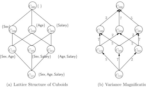
(a) Lattice Structure of Cuboids
C110 C101 C011 C111 C100 C010 C001 C000 7 2 2 7 5 5 7 2 5 2 7 5 (b) Variance Magnification
Figure 3.1: Lattice of cuboids and variance magnification of noise
Theorem 3.2.2 Kbase is²-differentially private. For any published cell a, E [˜c(a)] =c(a). If
ais in a cuboid with dimensions[C], the mean squared error isVar [˜c(a)] = 2QAj∈/[C]|Aj|/²2.
Proof: Since only the base cuboid is computed from T, the sensitivity S(Fbase) = 1. So
from Theorem 2.1.1, publishingFbase(T) +hLap(1/²)isatisfies²-differential privacy. For any
other cell a not in the base cuboid, the computation of ˜c(a) takes the released base cuboid as input, so from the composition property [59], is²-differentially private. For a cella in the base cuboid, E [˜c(a)] = E [c(a) + Lap(1/²)] = c(a), and Var [˜c(a)] = 2/²2. For a cell a in a cuboid C, it aggregates a set {a0}of Q
Aj∈/[C]|Aj|cells in the base cuboid. So we have
E [˜c(a)] = E " X a0 ˜c(a0) # =X a0 E [˜c(a0)] = X a0 c(a0) =c(a),
and since noise is generated independently,
Var [˜c(a)] = Var
" X a0 ˜c(a0) # =X a0 Var [˜c(a0)] = Y Aj∈/[C] |Aj| ·2/²2. 2
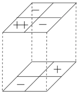
Example 3.2.1 For the fact table T in Figure 1.1(a), Figure 3.1(a) shows the lattice of cuboids under the relationship ¹. Three dimensionsSex, Age, and Salary have cardinality 2, 7, and5, respectively. Each cuboid is labeled as Cx1x2x3, where xi = 1 iff theith dimension is
in this cuboid. For example,C011 is the cuboid {Age,Salary}. The label on an edge from C to C0 in Figure 3.1(b) is the variance magnificationratio when cells in cuboid C are aggregated
to compute the cells in C0. For example, if C
011 is computed from C111, the noise variance doubles, since the dimension Sex has 2 distinct values–each cell in C011 is the aggregation of 2 cells in C111. If C001 is computed from C111, the noise variance is magnified 2×7 = 14 times, since 14 cells in C111 form one in C001.
Suppose we want to publish all the cuboids in Figure 3.1(a). Using Kall, we add Laplace
noise Lap(8/²) to each cell, giving noise variance 2×64/²2 = 128/²2 for one cell. Using Kbase, we add Laplace noise Lap(1/²) to each cell in C111 and then aggregate its cells. Each cell in C100 is built from7×5cells in C111, with noise variance 35×2/²2 = 70/²2. A cell in C000 is built from 7×5×2 cells in C111, with noise variance 70×2/²2 = 140/²2.
A better approach is to compute cuboidsC111, C110, C101, andC100 fromT, adding Laplace noise Lap(4/²)to each (the sensitivity is 4). We compute the other cuboids from these, which does not violate differential privacy as we do not touch the fact table. Then the noise variance in C100 is 32/²2 and in C000 is 2×32/²2 = 64/²2 (aggregating 2 cells of C100).
Example 3.2.1 shows that the more initial cuboids we compute from the table T, the higher their sensitivity is (more noise), but the less noise is accumulated when other cuboids are computed from them. Kall and Kbase are the two extremes of computing as many or as
few cuboids as possible directly from T. There is some strategy between Kall and Kbase that
gives better bounds for the noise variance of released cuboids. There are two intuitive ideas: the first is to vary the set of initial cuboids (C111, C110, C101, and C100 in Example 3.2.1); and the second is more general: we can vary the amounts of noise inserted into different initial cuboids. These two ideas will be elaborated in the rest of Sections 3.2 and 3.3, respectively.
3.2.1
Noise Control Framework: Cuboid Selection
We first introduce the framework of a better algorithm Kpart in this subsection. To publish
a set L ⊆ Lall of cuboids, Kpart chooses which cuboids, denoted as Lpre, to compute directly
from the fact table T, in a manner that reduces the overall noise. Lpost =L − Lpre includes
all the other cuboids in L. We do notrequire Lpre⊆ L. Kpart works as follows.
1. (Noise Sources) For each cell a of cuboids in Lpre, Kpart computes c(a) from T but
releases ˜c(a) =c(a) + Lap(s/²), where the sensitivitys=|Lpre|. Lpre is selected by our
algorithms in Section 3.2.2 s.t. all cuboids in L can be computed from Lpre.
2. (Aggregation) For each cuboid C ∈ Lpost, Kpart selects a descendant cuboid C∗ from
Lpre s.t. C∗ º C, and computes ˜c(a) for each cell a ∈ C by aggregating the noisy
measure of cells in C∗. We discuss how to pick C∗ as follows.
The measure ˜c(a) output by Kpart is an unbiased estimator of c(a) for every cell a,
i.e., E [˜c(a)] = c(a). For a cell a in cuboid C0 ∈ L
pre, Var [˜c(a)] = 2s2/²2 (s = |Lpre|).
Suppose cell a in C ∈ Lpost is computed from C0 ∈ Lpre by aggregating on dimensions
[C0]−[C] = {A
k1, . . . , Akq}, the variance magnificationis defined as
mag(C, C0) = Y 1≤i≤q
|Aki|. (3.1)
So the noise variance, the mean squared error, of ˜c(a) is
Var [˜c(a)] = mag(C, C0)·2s2/²2. (3.2)
Let mag(C, C) = 1. If C cannot be computed from C0, let mag(C, C0) = ∞. We should
minimal, i.e., mag(C, C∗) = min
C0∈Lpremag(C, C0). Let
noise(C,Lpre) = min
C0∈Lpremag(C, C
0)·2s2/²2 (3.3)
be the smallest possible noise variance when computingCfrom a single cuboid in the selected cuboid setLpre. In a special case, ifC0 ∈ Lpre, noise(C0,Lpre) = 2s2/²2.
Theorem 3.2.3 Kpart is ²-differentially private. For any released cell a, E [˜c(a)] =c(a).
Proof: The proof is similar to the one of Theorem 3.2.2. Consider the measures hc(a)i for all cells in thes selected cuboids inLpre, the sensitivity of publishingLpre is s=|Lpre|(since
the measure of exactly one cell in each cuboid in Lpre is changed by±1 if adding/deleting a
row inT). So by Theorem 2.1.1 and the composition property of differential privacy, adding a noise Lap(s/²) to each cell in Lpre and computing L from Lpre is ²-differentially private.
E [˜c(a)] =c(a) is also from the linearity of expectation. 2
Example 3.2.2 Consider the data cube in Example 2.1.1 and release algorithm Kpart with
Lpre ={C111, C110, C101, C100}. C000 can be computed fromC100 with noise variance2×32/²2, since mag(C000, C100) = 2; or from C110 with noise variance 14× 32/²2 = 448/²2, since mag(C000, C110) = 2×7 = 14. So Kpart chooses the best among all cuboids in Lpre, and
computes C000 from C100. And we have noise(C000,Lpre) = 64/²2.
Kpart shares some similarities to the matrix mechanismin [51]. Kpart chooses cuboids Lpre
to computeL, while [51] chooses a set of queries to answer a given workload of count queries. If we adapt [51] for our problem by treating a cell as a count query, we need to manipulate matrices of sizes equal to the number of cells (e.g., matrices with 106 ×106 entries for a moderate data cube with 106 cells). So [51] is not directly applicable in our context.
Efficient Implementation of Kpart. Suppose Lpre is given. A naive way to compute
C ∈ L, query its nearest descendant C∗ ∈ L
pre, and aggregate cells in C∗ to computeC.
We can compute differentially private cuboids inLmore efficiently with fewer cell queries. Suppose C ¹ C00 ¹ C∗, noise is injected into C∗ ∈ L
pre for ensuring differential privacy,
and C00 is computed from C∗. Then computing C from C∗ is equivalent to computing
it from C00, with differential privacy ensured. So after noise is injected into all cuboids
in Lpre, differentially private cuboids in L can be computed in a level-by-level way, i.e.,
computing i-dim cuboids from (i + 1)-dim cuboids. The total running time is O(Nd2), where N = Πj(|Aj|+ 1) is the total number of cells.
Cuboid selection problems: optimizing noise source Lpre
We formalize two versions of the problem of choosing Lpre with different goals, given table
T and setL of cuboids to be published.
Problem 1 (Bound Max) Choose a set Lpre of cuboids s.t. all cuboids in L can be
com-puted from Lpre and the max noise noise(Lpre) = maxC∈L noise(C,Lpre) is minimized.
Problem 2 (Publish Most)Given thresholdθ0 and cuboid weightingw(·), chooseLpre s.t.
P
C∈L: noise(C,Lpre)≤θ0w(C) is maximized. In other words, maximize the weight of the cuboids computed from Lpre with noise variance no more than θ0.
Theorem 3.2.4 The two cuboid selection problems Bound Max and Publish Most are
both NP-hard, if we treat |L| as the input size.
Proof: To complete the proof, we reduce the problem of Vertex Cover in degree-3 graphs to the Bound Max problem. Then the hardness ofPublish Most follows. Construction of Instances. Following is an instance of theVertex Coverproblem in a degree-3 graph (where the degree of a vertex is bounded by 3). Given a degree-3 (undirected) graph G(V, E) where|V|=n, decide ifG has a vertex cover V0 ⊆V with at most m (< n)
vertices. V0 ⊆ V is said to be a vertex cover of G iff for any edge uv ∈ E, we have either
u∈ V0 or v ∈ V0. Abusing the notations a bit, let cov(v) be th