A Utility-Based Approach
By LJ Rossouw ABSTRACT
The paper aims to investigate how much life insurance protection cover a utility maximising individual should buy. This question is relevant in the insurance industry as “best advice” in the sales process continues to be high on the agenda. The paper investigates this by modelling a family unit and maximising the expected future utility with optimal values of consumption and insurance spend. The optimal values are generally lower than those obtained by traditional methods of discounting of future earnings.
KEYWORDS
Life insurance; savings; consumption; utility ACKNOWLEDGEMENTS
The author would like to thank the following people who provided valuable comments and input to the paper: Paul Lewis, Peter Temple, Karl Steenkamp and Lorna McLaren.
CONTACT DETAILS
Rossouw, Louis, Gen Re, 9 Temasek Boulevard, #10-01 Suntec Tower 2, Singapore 038989, Singapore. Tel: +65 6438 7719. E-mail: lrossouw@genre.com
1
Introduction
Deciding on the level of insurance cover needed is not a simple decision to make from the point of view of the prospective policyholder. The prospective policyholder is asked to pay money for an intangible and uncertain future benefit foregoing immediate consumption or savings.
A typical solution to determine the level of cover required is to discount the portion of the insured’s expected future earnings to be spent on his or her dependants. This typically results in an aged based multiple that can be used as a guide to the decision making process.
A problem with this approach is that it does not take account of the fact that resources used for insurance could also be used for other uses. In this paper savings and consumption are considered as alternatives to insurance. Utility theory is the ideal tool for this and much research has already been done on consumption-savings models based on a utility approach. This general approach was started by Deaton (1991) and developed further by various authors including Carroll (1992 & 1997).
This paper extends the general approach to include insurance. To do this requires knowledge of the utility of assets after death. The model used in this paper considers the expected future utility of a family (as opposed to an individual). This gives the model the ability to measure the utility of assets left after the death of individual family members. The measure of utility used is the utility of consumption of those assets by the remaining family members. Hurd (1989) considered the marginal utility of bequests more directly which is not considered here.
Results are shown under various family structures and also for variations in some of the assumptions. The results are then discussed in the context of insurance products available in the market today. The assumptions used in this model borrow heavily from McCarthy (2005) and generally apply to the UK context. However other than the mortality and the income levels used, the assumptions and the model has been left relatively generic to allow for broader application.
2
The Model
The model evaluates the consumption, insurance purchase and savings decisions of a family unit, using a utility based approach. The model and its solution follows the general approach started by Deaton (1991), further developed by various authors including Carroll (1992 & 1997). The model and assumptions used here also draw heavily from McCarthy (2003 & 2005).
These models were done at the level of an individual. The proceeds of life insurance, by definition, cannot be consumed by the individual on whose life the policy was taken. Therefore, to include a measure of the utility of life insurance, modelling is done at the family level. This allows the utility of consumption of the insurance proceeds to be assigned utility in this model.
The model keeps track of the family’s assets as a whole and decisions are made to maximise the utility for the family as a whole. The family is modelled to consist of up to two potential income earners (referred to as parents or principal and spouse) and up to two dependents (referred to as children). It would be simple to extend the model to more dependents including adult dependents.
2.1
Utility function
It is assumed that each individual 𝑖 in the family has a utility at time 𝑡 that can be calculated by: 𝑢𝑖 𝐶
𝑡𝑖 =(𝐶𝑡
𝑖)1−𝛾 𝑖
1−𝛾𝑖 where 𝛾𝑖≥ 1
𝐶𝑡𝑖 is the consumption of the individual time 𝑡.
𝛾𝑖 is therefore the individual’s coefficient of relative risk aversion. Higher values of 𝛾𝑖 imply that individuals would value risky cash flows less than they would for lower values of 𝛾𝑖.
However, the model does not explicitly estimate the consumption for each individual at each future point. The model estimates consumption for the family as a whole. Given this level of consumption 𝐶𝑡, it is assumed that this consumption will be shared in fixed proportions amongst the members of the family. The same risk preference parameter for all family members is assumed (this means 𝛾𝑖 = 𝛾). Given 𝐶𝑡 and given that individual 𝑖 is alive, it is assumed that he or she would consume the following:
𝐶𝑡𝑖 = 𝐶
𝑡∙
𝑤𝑖 𝐿𝑗 𝑗𝑡𝑤𝑗
𝐿𝑗𝑡 is an indicator variable indicating whether life 𝑗 is alive at time 𝑡 (𝐿𝑡𝑗 = 1 being alive and 𝐿𝑡𝑗 = 0 for dead).
𝑤𝑗 represents the proportions in which consumption is shared between the family members. Thus the utility for the family at time 𝑡 can be expressed as
𝑢 𝐿 , 𝐶𝑡 𝑡 = (𝐶𝑡𝑖)1−𝛾 1 − 𝛾 𝑎𝑙𝑖𝑣𝑒 𝑖 =𝐶𝑡 1−𝛾 1 − 𝛾∙ 𝐿𝑖𝑡𝑤 𝑖 𝐿𝑗 𝑡𝑗𝑤𝑗 𝑖
𝐿𝑡 represents the specific combination of lives that are alive at time 𝑡.
The assumption of constant risk preference amongst the family members was useful to simplify the utility function. It could be argued that different members of the family would have different risk preferences. For example, parents and children may have different risk preferences and therefore different utility functions. However in this case the family, as a whole, is making a combined decision and the actual risk preferences of children are not considered. It may in fact be that the parents would feel that they need to be more cautious with regard to the children and therefore the risk preference should be lower. Given the uncertainty of setting the risk preference in any event it was left as a constant for all family members.
Children are also assumed to become independent at age 21 removing them from the model (equivalent to assuming that they die at this age).
Note that, in this paper, other motives for insurance are not allowed for. This paper therefore does not analyse insurance purchased based on a motive to leave a specific bequest to an individual.
2.2
Assets before consumption occurs and before insurance premiums are
paid
Development of the assets from time 𝑡 − 1 to time 𝑡 can be described by the equation below. 𝐴𝑡+1= 𝑅𝑡∙ 𝐴′𝑡+ 𝐿0𝑡+1∙ 𝐼
𝑡+10 ∙ 𝜃𝑡+10 + 𝛼0∙ 𝑌𝑡+1 + 𝐿1𝑡+1∙ 𝐼𝑡+11 ∙ 𝜃𝑡+11 + 𝛼1∙ 𝑌𝑡+1 +𝐷𝑡+10 ∙ 𝑆
𝑡+10 + 𝐷𝑡+11 ∙ 𝑆𝑡+11
Here 𝐴𝑡+1 represents the assets at time 𝑡 + 1 before insurance premiums are deducted or consumption occurs.
𝐴′𝑡 represents the assets at time 𝑡 after any insurance premium or consumption. 𝑅𝑡 represents the return on a risky portfolio of assets from time 𝑡 to time 𝑡 + 1. 𝐿𝑖𝑡+1 is an indicator variable indicating whether life 𝑖 is alive at time 𝑡 + 1 (𝐿
𝑡+1
𝑖 = 1 being alive and 𝐿𝑖𝑡+1= 0 for dead)
𝐼𝑡+1𝑖 is the expected income of life 𝑖 during the year ending at time 𝑡 + 1 (payable at the end of the year given that the life is alive at the end of the year).
𝜃𝑡+1𝑖 is the independent random income shock of life 𝑖 during the year ending at time 𝑡 + 1. Permanent shocks to income were not included as was done by McCarthy (2005). Also note that income shocks were assumed to be independent of the asset returns. McCarthy allowed for correlations in asset returns and income shocks.
𝐷𝑡+1𝑖 = 𝐿 𝑡
𝑖 − 𝐿
𝑡+1
𝑖 which indicates whether life 𝑖 has died in the year ending at time 𝑡.
𝑌𝑡+1 represents the joint annuity payable at time at time 𝑡 + 1 if both parents are alive at that point. If only the first life is alive then 𝛼0∙ 𝑌𝑡+1 is payable. If only the second is alive then 𝛼1∙ 𝑌𝑡+1 is payable. We use 𝛼0= 𝛼1 = 0.5 in this paper.
𝑆𝑡+1𝑖 represents the sum assured payable at time 𝑡 + 1 should the life 𝑖 die during the year ending at time 𝑡 + 1.
2.3
Annuitisation
To model the savings element more accurately, the model allows for annuitisation at retirement. Annuitisation was assumed to occur where no further income from either of the male or female lives is expected. This is similar to assuming that annuitisation occurs when the youngest parent reaches 65. Thus annuitisation occurs at the time 𝑡, where 𝐼𝑡0+ 𝐼𝑡1> 0 and 𝐼𝑢𝑖 = 0 for all 𝑢 > 𝑡. The single premium at time 𝑡 is:
𝑆𝑃𝑡=2 3𝐴𝑡 𝑌𝑡+1 = 𝑆𝑃𝑡
𝑎𝑡(1 + 𝑙)
𝑎𝑡 is an annuity factor representing the present value of an annuity of 1 payable in arrears on the lives of the parents. It reflects the 𝛼𝑖 and is automatically adjusted depending on who is alive at time 𝑡 and is discounted at the risk free rate of return. 𝑙 is the insurer’s margin.
Annuitisation of two-thirds of assets is assumed as this is a typical portion of pension assets that are required to be annuitised by authorities. It would also be possible to make the annuity decision open to optimisation.
Note that 𝑌𝑡 is included in the formulae below but it can be taken that 𝑌𝑡= 0 before retirement. This is done to keep the formulae in a more general form.
Note that modelling is done in real terms and that a level annuity here implies an annuity that compensates for inflation.
2.4
Insurance premium
𝑆𝑡𝑖 = 𝑃𝑡𝑖 𝑞𝑡𝑖/(1 − 𝑚)
Where 𝑚 represents the insurance margin (inclusive of allowance for discounting). 𝑞𝑡𝑖 is the mortality rate for life 𝑖 .
This paper only solves for 𝑃𝑡0 and assumes no insurance on the second parent (𝑃
𝑡1 = 0). This is equivalent to a one year term insurance. This paper uses 𝑞′𝑡 to represent 𝑞𝑡0/(1 − 𝑚) in equations below.
2.5
Assets after consumption and after insurance premiums are paid
This can now be expressed as:𝐴′𝑡 = 𝐴𝑡− 𝑆𝑃𝑡− 𝐶𝑡− 𝑃𝑡0 Here 𝑆𝑃𝑡 = 0 for all 𝑡 other than the year of retirement.
The full equation for the development of assets from time 𝑡 − 1 to 𝑡 becomes: 𝐴𝑡+1 = 𝑅𝑡∙ 𝐴𝑡− 𝑆𝑃𝑡− 𝐶𝑡− 𝑃𝑡0 +𝐿0𝑡+1∙ 𝐼 𝑡+10 ∙ 𝜃𝑡+10 + 𝛼0∙ 𝑌𝑡+1 +𝐿1𝑡+1∙ 𝐼 𝑡+11 ∙ 𝜃𝑡+11 + 𝛼1∙ 𝑌𝑡+1 +𝐷𝑡+10 ∙ 𝑆𝑡+10
Note the term 𝐷𝑡1∙ 𝑆𝑡1 has been removed as insurance on the second parent is not considered in this paper.
2.6
Implications of model choice
There are several implications of the model choice with regard to insurance risk.
The model is based on one year insurance cover only. This means that the paper does not take account of insurance cover over multiple years. Allowing for multi-period cover (with level premiums) as is typically available would need to allow for the potential for the individual’s health to deteriorate over time. This would require taking account of the underwriting process in some form. It would also need to allow for a choice in possible terms of cover and allow for the potential of lapse\surrender. Including this level of detail would be very complex. This would add value to the model as optimal choices could be considered given products available in the market.
This simple approach has the advantage of allowing the development of an understanding of the true insurance need in each year. However, this is in the absence of potential future ill-health that would accelerate the need for cover to earlier ages. Another way to interpret the model is to view this as the
cover needed in an employer based group policy where the impact of individual underwriting is of lesser concern.
Other model features that have been simplified when compared to McCarthy (2005) are the fact that the income shock is independent of asset returns. McCarthy (2005) was investigating the impact of asset choice and it was important that correlations between the risky asset and income choice be allowed for. Here asset mix is constant.
Children are also assumed to become independent at age 21. This means that after this point, any assets left after both parents die have no utility. It could be argued that these assets would still have some utility to any children and/or other relatives who receive these assets at this point. The utility would however be lower than that of a dependent child/relative.
Credit related insurance protection is not covered by this model.
Permanent/persistent impact shocks have not been modelled. One would expect this to result in underestimation of the level of savings earlier in life as this element is likely to provide the biggest uncertainty to the individual. Understating the savings may mean that insurance premium spend is overstated.
3
Solving the model
The problem can be defined as finding the values of 𝐶𝑡 and 𝑃𝑡0 such that following is maximised: 𝐸 𝑣𝑡𝑢(𝐿 𝑡 , 𝐶𝑡) 𝑇 𝑡=0
In words, this means that the problem is to choose future consumption and insurance premiums such that the discounted future utility is maximised. Expectation is taken with regard to income shocks, asset returns, as well as potential future values of Lt.
T is chosen such that no life is expected to survive beyond T or qTi = 1 for all i.
Here v is a discounting factor at rate of time preference of consumption. This is a rate reflect the family’s preference for consumption, usually set such that earlier consumption is preferred. By defining 𝑉𝑡 𝐿 𝑡, 𝐴𝑡, 𝑌𝑡 = max 𝐶𝑡,𝑃𝑡0 𝐸 𝑣𝑠−𝑢𝑢(𝐿 𝑠, 𝐶𝑠) 𝑇 𝑠=𝑡 The problem can then be written as:
𝑉𝑡 𝐿 𝑡, 𝐴𝑡, 𝑌𝑡 = max 𝐶𝑡,𝑃𝑡0 𝑢 𝐿 𝑡, 𝐶𝑡 + 𝐸 𝑣𝑠−𝑢∙ 𝑢 𝐿 𝑠, 𝐶𝑠 𝑇 𝑠=𝑡+1 This can be expressed as:
𝑉𝑡 𝐿 𝑡, 𝐴𝑡, 𝑌𝑡 = max
𝐶𝑡,𝑃𝑡0
𝑢 𝐿 𝑡, 𝐶𝑡 + 𝑣 ∙ 𝐸 𝑉𝑡+1 𝐿 𝑡+1, 𝐴𝑡+1, 𝑌𝑡+1
Equation 1
3.1
Derivatives
To solve for 𝐶𝑡 in Equation 1, we differentiate with regard to 𝐶𝑡 we get the following equation: 𝑢𝐶 𝐿 𝑡, 𝐶 𝑡 − 𝑣 ∙ 𝐸 𝑅𝑡∙ 𝑉𝑡+1𝐴 𝐿 𝑡+1, 𝐴𝑡+1, 𝑌𝑡+1 = 0 Giving us: 𝑢𝐶 𝐿 𝑡, 𝐶 𝑡 = 𝑣 ∙ 𝐸 𝑅𝑡∙ 𝑉𝑡+1𝐴 𝐿 𝑡+1, 𝐴𝑡+1, 𝑌𝑡+1 Equation 2 Where 𝑢𝐶 represents differentiation of 𝑢 with regard to the second parameter and 𝑉𝑡+1𝐴 represents the differentiation of 𝑉𝑡+1 with regard to the second parameter.
Broadly speaking, the envelope theorem states that the differential of a maximum value of a function is the differential of the function evaluated at the other parameters which maximise it. Using the
envelope theorem, 𝑉𝑡𝐴 𝐿
𝑡, 𝐴𝑡, 𝑌𝑡 must equal the differential with regard to 𝐴𝑡 of the RHS of Equation 1 evaluated at 𝐶 𝑡.
𝑉𝑡𝐴 𝐿
𝑡, 𝐴𝑡, 𝑌𝑡 = 𝑣 ∙ 𝐸 𝑅𝑡∙ 𝑉𝑡+1𝐴 𝐿 𝑡+1, 𝐴𝑡+1, 𝑌𝑡+1
Equation 3 Using Equation 2 and Equation 3 we have that:
𝑉𝑡𝐴 𝐿 𝑡, 𝐴𝑡, 𝑌𝑡 = 𝑢𝐶 𝐿 𝑡, 𝐶 𝑡 Equation 4 Alternatively: 𝑉𝑡+1𝐴 𝐿 𝑡+1, 𝐴𝑡+1, 𝑌𝑡+1 = 𝑢𝐶 𝐿 𝑡+1, 𝐶 𝑡+1 Thus we can update Equation 2 to the following:
𝑢𝐶 𝐿
𝑡, 𝐶 𝑡 = 𝑣 ∙ 𝐸 𝑅𝑡∙ 𝑢𝐶 𝐿 𝑡+1, 𝐶 𝑡+1
Equation 5 This is the Euler equation for consumption.
Solving for 𝑃𝑡 involves differentiating the RHS of Equation 1 with regard to 𝑃𝑡. This gives us: 𝑣 ∙ 𝐸 𝐷𝑡+1 0 𝑞′𝑡 − 𝑅𝑡 ∙ 𝑉𝑡+1𝐴 𝐿 𝑡+1, 𝐴𝑡+1, 𝑌𝑡+1 = 0 Or 𝑣 ∙ 𝐸 𝐿0𝑡− 𝐿0𝑡+1 𝑞′𝑡 − 𝑅𝑡 ∙ 𝑉𝑡+1 𝐴 𝐿 𝑡+1, 𝐴𝑡+1, 𝑌𝑡+1 = 0 Using Equation 4 we have that:
𝑣 ∙ 𝐸 𝐿𝑡 0− 𝐿 𝑡+1 0 𝑞′𝑡 − 𝑅𝑡 ∙ 𝑢 𝐶 𝐿 𝑡+1, 𝐶 𝑡+1 = 0 Equation 6
3.2
Solving
Broadly speaking, the approach to solving this problem involves noting that 𝐶 𝑇 = 𝐴𝑇 and 𝑃 𝑇 = 0 as all assets should be consumed in the last period and insurance should not be needed. Using this fact
and solving Equation 5 and Equation 6 simultaneously we can solve for 𝐶 𝑇−1 and 𝑃 𝑇−1. This can then be extended further to solve all 𝐶 𝑡 and 𝑃 𝑡.
In practice similar methods were used as those described in McCarthy (2003 & 2005) and Carroll (1992). Carroll (Unpublished) gives a more detailed description of the type of work involved.
This involves in solving 𝑃 𝑡 and 𝐶 𝑡, successively. We assume that we have already solved
𝐶 𝑡+1 𝐿 𝑡+1 , 𝐴𝑡+1, 𝑌𝑡+1 for all 𝐴𝑡+1 and 𝑌𝑡+1. Here 𝐴𝑡+1 is presumed to be after any annuity premium has been deducted. Similarly we assume we have already solved 𝑃 𝑡+1 𝐿 𝑡+1 , 𝐴𝑡+1, 𝑌𝑡+1 . In this case 𝐴𝑡+1 should be after the relevant single premium and 𝐶 𝑡+1.
We can then solve 𝑃 𝑡 that satisfies: 𝑣 ∙ 𝐸 𝐿𝑡 0− 𝐿 𝑡+1 0 𝑞′𝑡 − 𝑅𝑡 ∙ 𝑢𝐶 𝐿 𝑡+1, 𝐶 𝑡+1 𝐿 𝑡+1 , 𝐴 𝑡+1, 𝑌 𝑡+1 = 0 Where 𝐴 𝑡+1= 𝑅𝑡∙ 𝐴𝑡− 𝑃 𝑡 +𝐿0𝑡+1∙ 𝐼 𝑡+10 ∙ 𝜃𝑡+10 + 𝛼0∙ 𝑌𝑡+1 +𝐿1𝑡+1∙ 𝐼 𝑡+11 ∙ 𝜃𝑡+11 + 𝛼1∙ 𝑌𝑡+1 + 𝑃 𝑡 𝐷𝑡+10 𝑞′ 𝑡 − 𝑆𝑃𝑡+1
The above equation is solved using numerical methods for various values of 𝐴𝑡 and 𝑌𝑡 and for all possible 𝐿 𝑡 . A numerical method based on Brent (1973) was used to solve for 𝑃 𝑡. This method is essentially a mixture between the Bisection method and the Newton-Rhapson method. The resultant values are then used to construct the interpolating function 𝑃 𝑡 𝐿 𝑡 , 𝐴𝑡, 𝑌𝑡 .
Note that the distributions for 𝑅𝑡 and 𝜃𝑡+1𝑖 are used in approximate discrete form to speed up calculation as was done by Carroll and McCarthy.
We can then similarly solve for 𝐶 𝑡 using the interpolating function 𝑃 𝑡 𝐿 𝑡 , 𝐴𝑡, 𝑌𝑡 and the following equation:
𝑢𝐶 𝐿
𝑡, 𝐶 𝑡 = 𝑣 ∙ 𝐸 𝑅𝑡∙ 𝑢𝐶 𝐿 𝑡+1, 𝐶 𝑡+1 𝐿 𝑡+1 , 𝐴 𝑡+1, 𝑌 𝑡+1)
The fact that one can calculate the inverse function of 𝑢𝐶 directly helps to solve for 𝐶 𝑡. An interpolating function 𝐶 𝑡 𝐿 𝑡 , 𝐴𝑡, 𝑌𝑡 is then constructed as above.
The point values used to build the interpolating functions are chosen such that the values for 𝐴𝑡 and 𝑌𝑡 form a regular grid. The point values also specifically include values that satisfy the boundary conditions of 𝐶 𝑡 and 𝑃 𝑡. For example, 𝐶 𝑡 𝐿 𝑡 , 𝐴𝑡, 𝑌𝑡 = 𝐴𝑡 is a boundary condition for some values of 𝐴𝑡 and 𝑌𝑡.
Incorporating these values in the grid improves the accuracy of the numerical solutions. The end effect is that all values reflecting boundary conditions lie on intersections of the grid. This is useful for
interpolation.
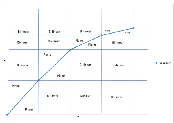
Interpolation of 𝐶 𝑡 𝐿 𝑡 , 𝐴𝑡, 𝑌𝑡 or 𝑃 𝑡 𝐿 𝑡 , 𝐴𝑡, 𝑌𝑡 with regard to 𝐴𝑡 and 𝑌𝑡 is accomplished using the following method. The box of the grid containing the particular 𝐴𝑡 and 𝑌𝑡 is determined. Bilinear interpolation is then used with regard to 𝐴𝑡 and 𝑌𝑡 and the four corners of the box. Where the values of 𝐴𝑡 and 𝑌𝑡 are in a grid box which has two values that lie on a boundary condition (on opposing corners), the box is split into two triangles and the triangle which contains the point is picked. Based on the values of the function at the three corners of the relevant triangle, the parameters of the plane that goes through these points is determined and the relevant interpolated value is determined using these parameters. Figure 1 illustrates this graphically. The function 𝐶 𝑡 or 𝑃 𝑡 is calcualted at all intersection of the grid lines and values for other 𝐴𝑡 and 𝑌𝑡 are then interpolated as shown.
Before retirement 𝑌𝑡 = 0 and a simple approach is adopted. Simple linear interpolation is used (but still including the relevant boundary value as appropriate).
4
Assumptions
The assumptions are taken mainly from McCarthy (2005) as applied in the UK context. These assumptions appear to be reasonable long term assumptions. The detailed assumptions are listed below. Deviations from McCarthy (2005) are indicated.
4.1
Family structure
The family is assumed to be made up of a principal life, spouse and dependents. In the base scenario, the principal is assumed to be a 30-year old male with a 28-year old female spouse. They are assumed to have two children (a male 3-year old and a 1-year old female). Variations to this structure are investigated.
McCarthy (2005) modelled an individual life only and therefore did not need to assume a family structure.
4.2
Risk preferences
Risk aversion was set as γ = 3 as per McCarthy (2005). Variations to this assumption are investigated. Higher values of γ imply that individuals would value risky cash flows less than they would for lower values of γ.
The time preference discount rate was set at 3% which indicates an impatience to consume compared to the risk free rate of 2%.
4.3
Sharing of consumption
The weights used to split consumption for individuals in the family are subjective. The following proportions were used:
Family member Share Principal 30%
Spouse 30%
Child 1 20%
Child 2 20%
Each parent was assigned 30%. This implies that, should both parents be alive, consumption would be equally shared between them. Each of the two children was assigned 20%. This implies an equal share of consumption amongst them.
These assumptions do not appear unreasonable in comparison to studies that have been done on this topic. (See United States Department of Agriculture (2007) which shows that in husband and wife families with two children 42% of expenditure is attributable to the children. Similarly where one child is present the figure is 26%.)
Insurance margins were set at 20%. Sensitivity testing was done around this assumption. The margin on the annuity is assumed to be 10%.
4.5
Income & Income Shocks
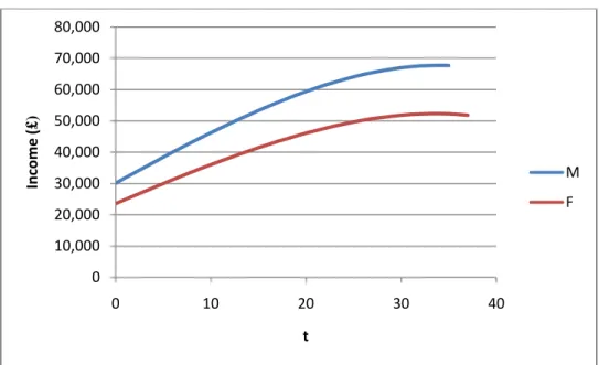
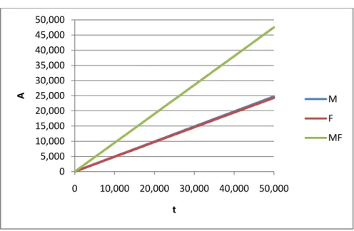
Income follows the income formulae supplied in McCarthy (2005) for individuals with a degree. McCarthy based these on the Labour Force Survey (LFS), March-May 2004, produced by the Office of National Statistics. This paper also includes the 1.5% p.a. productivity gain adjustment as was used by McCarthy. Figure 2 shows the income profile used for a male aged 30 and a female aged 28 at time 0. Throughout most of the paper it is assumed the male is the only income earner. In section 5.9 below a dual income family is analysed.
Figure 2 – Expected income for males and females in future time periods
𝜃𝑡+1𝑖 is assumed to be independently log normally distributed. The mean was set to 1 and the value of standard deviation of 20%. This is similar to McCarthy (2005) although this paper does not allow these shocks to persist over time.
4.6
Asset returns
Asset returns are given by:𝑅𝑡 = 𝛼 ∙ 𝜀𝑡− 1 + 𝑟 + 𝜇 + 1 − 𝛼 ∙ 𝑟
𝛼 represents the portion of assets invested in equity and is set at 65%. McCarthy (2005) left this parameter to be optimised as part of his model. Investigating asset mix was not one of the goals of this paper and it was therefore removed and set to a value that is typical for retirement related liabilities. 𝑟 represents the risk free real rate of return and was set at 2%. 𝑟 is also used as the discount rate in the calculation of the annuity (𝑎𝑡).
0 10,000 20,000 30,000 40,000 50,000 60,000 70,000 80,000 0 10 20 30 40 In co m e ( £) t M F
𝜇 represents the equity risk premium and was set at 5%.
𝜀𝑡 are assumed to be independently log normally distributed with mean of 1 and standard deviation of 20%.
4.7
Mortality
Mortality rates are taken from the tables provided in Office for National Statistics (2009). The tables for the United Kingdom, however, the model assumes 𝑞100 = 1. Note that a population mortality table was used as there no specific allowance was made for the impact of selection and underwriting in this analysis. Lives are assumed to be independent.
4.8
Tax
Income taxation and inheritance tax have been ignored in this analysis.
Income taxation would reduce the income and returns achieved on the assets. Inheritance or estate tax would increase the amount of insurance that need to be held.
5
Results
5.1
Consumption before retirement
Consumption before retirement is a function of the assets at hand and the lives that are alive at that point in time.
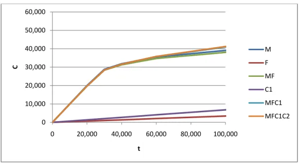
Figure 3 shows the consumption function at time 0 for various combinations of lives that are alive. M and F represents the presence of a male parent and female parent respectively. C1 and C2 represent the presence of the first and second child respectively. Here and for further analysis the male is the only income earner (unless stated otherwise).
If the male is alive it can be seen that the male would consume all his assets if they are below 20,000. It is possible for him to consume all his assets as he expects an income which will cover this. He is also expecting increasing income and can thus delay saving for retirement. This is a boundary condition. This condition only applies if just the male is alive and earning income.
Where both male and female are alive (with or without children) such a boundary condition does not occur. Some portion of assets would need to left after consumption in order to purchase insurance at these low levels of assets.
When only the female is alive no further income is expected and only a small portion of income is consumed, as the remaining assets are expected to last her lifetime. Similarly if only a child is alive consumption is limited. They can however consume more than the female as they are only consuming until they reach age 21.
Consumption is the greatest where the whole family is alive.
Figure 3: Optimal Consumption function at time 0 for various family structures and various values of assets.
0 10,000 20,000 30,000 40,000 50,000 60,000 0 20,000 40,000 60,000 80,000 100,000 C t M F MF C1 MFC1 MFC1C2
Figure 4 shows the same curves at time 20. If only a child is alive they would consume everything as they would be reaching 21. The female parent would still be consuming a small portion of her assets. If the male or the male and female are alive they would consume most of their assets if assets available fell below approximately 30,000 but would not consume significantly more than this if assets increased. Figure 4 – Optimal Consumption function at time 20 for various family structures and various values of assets.
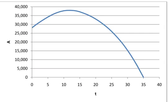
The boundary condition prior to retirement is shown in Figure 5. This condition only applies if just the male is alive. If assets at the time of consumption is equal or below the plotted value all assets will be consumed. The value increases for the first number of years as income increases.
Figure 5 – Boundary condition on consumption over time for the case where just the principal life is alive.
0 50,000 100,000 150,000 200,000 250,000 0 5 10 15 20 25 C t M F MF C1 MFC1 MFC1C2 0 5,000 10,000 15,000 20,000 25,000 30,000 35,000 40,000 0 5 10 15 20 25 30 35 40 A t
5.2
Insurance premium
One boundary condition for premiums is shown in Figure 6. If assets after consumption are below the level indicated all these assets will be used to purchase insurance. This increases over time as more free income is available to fund insurance premiums. It is also higher for couples without children.
Figure 6 – Boundary condition on insurance premium for various family structures over time.
No insurance is required after retirement because the annuity purchased is a joint life annuity. Figure 7 shows insurance premium for various combinations of remaining family members as well as various levels of assets at time 10. The premium is not very sensitive to assets available. As assets increase the optimal premiums would start reducing as the excess assets begin to negate the value of insurance.
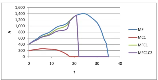
Figure 7 – Optimal insurance premium for various family structures and asset values at time 10.
0 200 400 600 800 1,000 1,200 1,400 1,600 0 10 20 30 40 A t MF MC1 MFC1 MFC1C2 0 100 200 300 400 500 600 700 800 900 1,000 0 10,000 20,000 30,000 40,000 50,000 P A MF MC1 MFC1 MFC1C2
5.3
Consumption after retirement
Figure 8 sets out consumption at time 40 (i.e. after retirement) given that both male and female are alive. Each line represents a different level of annuity payable. Where no annuity is payable a small portion of assets are consumed as the assets need to last the remaining lifetimes of the parents. Where an annuity is in payment consumption can be more aggressive. The chart also indicates the approximate boundary condition for consumption.
Figure 8 – Optimal consumption for various values of annuity and various asset values at time 40 (male and female alive).
Figure 9 shows the boundary conditions on consumption for various annuity values at time 40. Note that where the annuity is payable on a single life half the value indicated is being paid out. This explains the differences in the curves.
Figure 9 – Boundary condition on consumption at time 40 (male and female alive)
0 5,000 10,000 15,000 20,000 25,000 30,000 35,000 40,000 45,000 50,000 0 40,000 80,000 120,000 C A 0 10,000 20,000 40,000 0 5,000 10,000 15,000 20,000 25,000 30,000 35,000 40,000 45,000 50,000 0 10,000 20,000 30,000 40,000 50,000 A t M F MF
5.4
Estimated Sum Assured
Optimum sums assured from the model are compared to estimates of sum assured derived using traditional methods. These estimates were calculated as the present value of the male’s discounted income reduced by the fraction of the male’s consumption in each future year. Thus, if only the adults are present 50% of the income is discounted. If both parents and children are present 1 − 30% = 70% of the income is discounted. Children are only included up to age 21.
The discounting is done without adjustment for survival probabilities. Thus the estimated sum assured does not allow for the fact that the children or spouse may not live long enough to need the cover provided. For children this is not a significant difference but for the female this is more significant. Note that where the sum assured is expressed as a multiple of income, it is expressed as a multiple of the expected income payable at the end of that same year.
Thus the multiple is calculated as = 𝑆𝑡 𝐼
𝑡+10
5.5
Random Single Simulation
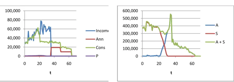
Figure 1 shows the income, annuity income, consumption and insurance premium of a single simulated family of 4. The volatility of income and asset returns can be seen. It can also be seen how
consumption is reduced after children reach aged 21. The annuity payments are also shown. It can be seen that one of the adults (the male) dies which results in a reduction of the annuity as well as consumption. Here A represents the assets and S the sum assured.
Figure 10 – Development of income, annuity income, consumption and insurance premium.
Figure 11 – Development of assets and sum assured for single simulation.
Figure 11shows the corresponding development of assets and sum assured over time. It also plots the sum of assets and sum assured. In this case it can be seen savings mainly occur after the children have reached 21. Here A represent assets and S the sum assured.
0 20,000 40,000 60,000 80,000 100,000 0 20 40 60 t Income Ann Cons P 0 100,000 200,000 300,000 400,000 500,000 600,000 0 20 40 60 t A S A + S
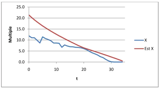
Figure 12 shows the multiple of income that is estimated (Est X) and the modelled multiple (X). It can be seen that early on (while the children remain dependants) the estimated multiple of income is not obtained.
Figure 12 – Optimal cover multiple and estimated cover multiple for family over single random simulation.
5.6
Averaging of simulations
To gain a more typical picture the process above was repeated a 1,000 times and the result averaged. For each simulation it was assumed that none of the lives died. This was done to allow a review of future insurance and consumption decisions and the resultant savings.
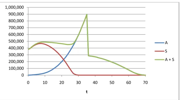
Figure 13 is an example of the results of such a simulation and shows the asset build-up and sum assured for a family consisting of only an adult male and female. As this is an average over many simulations values change smoothly over time. Figure 14 shows the consumption, income, annuity income and insurance premium for the same family.
0.0 5.0 10.0 15.0 20.0 25.0 0 10 20 30 M u ltiple t X Est X
Figure 13 – Average assets & sum assured for a couple with no children.
Figure 14 – Average income, annuity income, consumption and insurance premium for a couple with no children.
0 100,000 200,000 300,000 400,000 500,000 600,000 700,000 800,000 900,000 1,000,000 0 10 20 30 40 50 60 70 t A S A + S 0 10,000 20,000 30,000 40,000 50,000 60,000 70,000 80,000 0 10 20 30 40 50 60 70 t Income Ann Cons P
5.7
Comparison of results for various family structures
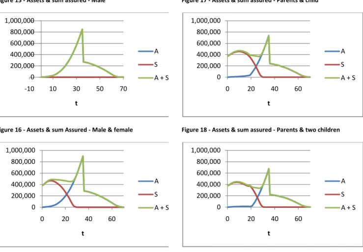
The four figures below show development of assets and sum assured for the various family structures.
Figure 15 - Assets & sum assured - Male
Figure 16 - Assets & sum Assured - Male & female
Figure 17 - Assets & sum assured - Parents & child
Figure 18 - Assets & sum assured - Parents & two children
Figure 19 shows how the average optimum amount of cover purchased in the model (designated “S”) compares with the estimates for the amount of cover required (designated “Est S”). Section 5.4 above describes how these estimates were derived. This is shown for three family structures which were simulated as above. As expected the estimate of cover required increases as members are added to the family. This is because the male is expected to consume a smaller proportion of his own income as he has to share it with other family members. Thus a larger portion of the present value of his income needs to be insured. Figure 20 shows the same information expressed as multiples of income. However there is limited increase in the cover purchased in the model. In fact less cover is purchased for the largest family structure than any of the other family structures. Figure 21 provides a possible explanation. Here it can be seen that the families with children have higher levels of consumption earlier on which limits the resources available for insurance premiums.
0 200,000 400,000 600,000 800,000 1,000,000 -10 10 30 50 70 t A S A + S 0 200,000 400,000 600,000 800,000 1,000,000 0 20 40 60 t A S A + S 0 200,000 400,000 600,000 800,000 1,000,000 0 20 40 60 t A S A + S 0 200,000 400,000 600,000 800,000 1,000,000 0 20 40 60 t A S A + S
Figure 19 – Optimum sums assured and estimated sums assured for various family structures.
Figure 20 - Optimal cover multiples for various family structures
0 100,000 200,000 300,000 400,000 500,000 600,000 700,000 800,000 0 10 20 30 S t MF S MF Est S MFC1 S MFC1 Est S MFC1C2 S MFC1C2 Est S 0 5 10 15 20 25 0 10 20 30 M u ltiple t MF Mult MF Est Mult MFC1 Mult MFC1 Est Mult MFC1C2 Mult MFC1C2 Est Mult
Figure 21 - Optimum consumption for various family structures.
5.8
“Unintended bequests”
Even though the model does not allow for a bequest motive these do arise unintentionally. Because of cautionary savings, the last individual of the family remaining (usually a parent as the children are excluded from the model at 21) would leave some assets for consumption in the next year resulting in a bequest should death occur in the current year. These assets have no utility in the context of the model. Figure 22 shows the average of assets left over on death of the last parent after retirement (from a starting family of four from a 1,000 simulations. These amounts are volatile as this is only a 1,000 simulations. However, these amounts are substantial given that annual consumption between time 40 and 50 is expected to be roughly 35,000 to 40,000 per year (given both parents are alive).
Figure 22 - “Unintended bequests” – The average amount of assets left on death of last parent at different times
0 10,000 20,000 30,000 40,000 50,000 60,000 70,000 -10 10 30 50 70 C t M MF MFC1 MFC1C2 0 50,000 100,000 150,000 200,000 250,000 300,000 350,000 400,000 35 45 55 65 A t
5.9
Dual income families
A family where both parents earn an income requires less insurance as illustrated in Figure 23 & Figure 24 (for a full family of four). Insurance is only modelled on the male life. There is limited reason for the female to require insurance on the male as she is earning an income too and would have recourse to that income (or savings based on that income) if the male died. There is some scope for insurance if the if one parent’s income is significantly above the other. Also insurance is required early on as the male is providing for children. The female also contributes to supporting dependents and would require insurance but this is not modelled.
Note that the assumption of independence would most likely result in an underestimation of insurance as the probability of the parents dying in the same event is underestimated.
Figure 23 – Assets & sum assured – Dual income Figure 24 – Assets & sum assured – Single income
5.10
Variation of risk preference
Figure 25 shows the impact of varying values 𝛾 in the utility function. Increasing 𝛾 results in more risk averse behaviour which, in turn, results in more insurance being purchased. Reducing 𝛾 has the opposite effect. 0 200,000 400,000 600,000 800,000 1,000,000 1,200,000 1,400,000 0 20 40 60 t A S A + S 0 200,000 400,000 600,000 800,000 1,000,000 1,200,000 1,400,000 0 20 40 60 t A S A + S
Figure 25 – Impact of varying 𝜸 on optimal sum assured for a family (two parents and two children)
5.11
Variation in insurance margin
Variations in the insurance margin assumption were also tested. Increasing the margin from 20% to 30% resulted in less cover being bought by a family of four. The reduction in cover was roughly 5% in most time periods. Time periods after 20 saw bigger reductions in percentage terms. Reducing the margin to 10% resulted in an approximate 4% increase in sum assured bought with bigger increases after time 20. Figure 26 - Impact of varying insurance margin on optimal sum assured for a family (two parents and two children)
0 50,000 100,000 150,000 200,000 250,000 300,000 350,000 400,000 450,000 500,000 0 10 20 30 40 S t γ =2 γ = 3 γ = 4 0 50,000 100,000 150,000 200,000 250,000 300,000 350,000 400,000 450,000 500,000 0 10 20 30 40 S t 10% 20% 30%
6
Discussion
6.1
Insurance gap
Studies in various markets have found large insurance “gaps”. The gaps tend to be measured between the ideal covers and the actual covers in the market. See Yee et al. (unpublished) for Singapore or Hugo & Zondagh (unpublished) in the case of South Africa for examples of this type of insurance gap analysis. The results here show that a potential reason for the gap is that consumptions and/or savings are prioritised. Specifically, families with children tend to prioritise consumption. It is also expected with more volatile income that savings will take some priority early on and would reduce the amount insured It is clear that additional work may be required to understand the alternatives to insurance.
Dual income families also seem to be important here. If our analysis included life insurance on both income earners it is expected the amount insured on each life would be closely related to the amount of cover required to allow the remaining parent to support the children at his or her salary until they become independent. Thus the amount of cover is actually quite small in this case.
6.2
Pattern of savings
Pattern of savings is not a fixed percentage of income over time. Optimal savings start off lower and accelerate in absolute and relative terms later. It would be ideal if individuals could save earlier for retirement but the reality seems to be that it would be somewhat easier to save more later in life when income is high and when children have become independent.
The asset build up over time in the absence of children were similar in shape to the results obtained by McCarthy (2003). Savings in this paper may be delayed, because income shocks aren’t modelled to be persistent. Simulations also mostly started from age 30 assuming no assets at that point whereas McCarthy (2003) started at age 20 allowing more time for savings to build up.
6.3
Life insurance products
From the analysis here the optimal cover seems to be a reducing multiple of income (in real terms) over time, ceasing near retirement. Cover is then generally not needed after this point in time (unless a single life annuity is purchased).
In the absence of allowance for funeral costs and bequests, protection products with level sums assured (real or nominal) may result in over insurance in later periods. Products with a limited term should be preferred over products that are whole of life.
A family income benefit would seem to be a reasonable option in terms of shape of cover (especially if the benefit is expressed in real terms) and also if the individual can increase cover after the initial purchase.
Figure 16 shows the optimal asset and cover development for a couple without children. A unit-linked policy with a sum assured of 400,000 to 500,000 (in real terms), where the death benefit is the sum assured or value of the units, would not seem to be an unreasonable choice to replicate this
development pattern. From a savings perspective a product that allows accelerating savings later in the term of the product would also seem useful.
Level premium whole of life products do not seem to be justified in terms of the amount of cover in later life. By paying a level premium the individual would be paying for protection which they would not need in later life. If surrender benefits are realistic or premiums increase following the risk (i.e.
increases more in line with mortality increases) this problem would be reduced as the individual could lapse\surrender cover that is not required at a later time. This type of cover would make more sense for some bequest motives and for paying inheritance tax on key assets.
Group life cover that is a fixed multiple of salary would seem less appropriate. An age based multiple would seem more appropriate to the need.
There do not seem to be products that perfectly fit the type of insurance protection needed as
described here (ignoring bequest and other motives for insurance not analysed in this paper). This may be an area requiring further innovation in product development.
6.4
Shortcomings of the model
Deciding on how consumption is prioritised inside the family is somewhat subjective. Here consumption is split in fixed proportions. Another method may involve individual utility functions and allocating consumption in the family based on equating marginal utilities. This may seem more objective in that an ad-hoc division of consumption is avoided but this would require a specific risk preference assumption for each member of the family.
The fact that permanent impacts to income were not allowed for means that too much confidence is placed on future earnings ability resulting in savings that are probably too low early on. This means that little is saved in early periods (as consumption seems to take precedence). This was done to keep the model relatively simple as adding this effect would require an additional variable which would increase complexity and running time. It is expected that adding this effect would result in reduced level of insurance as savings would become relatively more important.
The results in this paper mainly focuses on the situation where only one parent is earning an income. However it is likely that the other parent will be providing household services which will need to be replaced on his or her death. These services are not valued here explicitly but would need to be taken account if insurance on the spouse is modelled.
Bequest motives, other than utility of dependents’ consumption of assets, were ignored from this analysis. Individuals may feel compelled to leave some inheritance to relatives/children even if they are not dependant on the individual. We have, however, shown that substantial bequests do still arise in the model as a consequence of cautionary saving.
The mix of assets is assumed to be constant over time. Typically assets are expected to be invested more conservatively as the individual approaches and enters retirement. See McCarthy (2003 & 2005) for analysis that shows optimal choices of a mix of equities and the risk free assets.
More generally the assets are limited to equities and risk free assets. In practice many individuals own their homes and may have other assets. The paper also does not explicitly allow for home ownership and the associated mortgage term assurances. Implicitly it is assumed that living expenses will be adjusted to the means available. Thus, if a death results in mortgage payments no longer being affordable, the home would be sold and new smaller home would be bought (or rented). In practice individuals often prefer to have mortgage insurance in place which would avoid this problem. This could be considered a specific bequest motive. Another way to consider the home is to consider it as a special asset class with mortgage insurance as the cost of securing the asset in case of death.
6.5
Further research
Research should be extended to allow for health deterioration and multiple year cover. This would allow investigating current product types available in the market and would allow us to conclude amounts of cover to be purchased and the timing of these purchases. It would also allow the
investigation on when it may be optimal to lapse products from the insured’s perspective. A suggested course of action would be to model a simple whole of life product. Various premium patterns and surrender benefits could then be investigated. This would allow the model to be extended to allow for health status, without complicating it by allowing the choice of products of different terms. A fair surrender benefit (or premiums increasing with mortality) would remove the disadvantages of whole life cover.
Other insurable risks that require analysis are health insurance and disability insurance. These could be included in a future model. If disability is to be included, income profile and volatility assumptions may require adjustment as these may implicitly allow for some income volatility due to disability.
The amount of annuitisation could be allowed for as a variable to be optimised at retirement (as was done by McCarthy (2003 & 2005)), but also potentially throughout projection. It is expected that some annuitisation would be optimal after death of the income earner. Preliminary work has been done on a model of this form, which does show this.
7
Conclusion
This paper extends the typical consumption-savings utility models introduced by Deaton (1991) to include insurance. This is accomplished by modelling utility for the family unit giving the model the ability measure the utility of consumption after death of the insured and thereby optimising the insurance purchasing decision. This is shown to be a useful method to assess the optimal choice of insurance in the presence of the alternatives of savings and consumption.
Even though the model is simplified and has some limitations it provides a useful framework to review the insurance decisions of a utility maximising family. It also allows the assessment of possible reasons for cover being below the “ideal” discounted earnings approaches that are used today. It also allows the comparisons of the suitability cover provided in existing products compared to the optimal cover
patterns produced by the model.
Further research could improve this model, for example, to allow assessment of the amount of cover to be purchased and the timing of the purchase in the presence of the potential for deteriorating health as well as for other risks such as disability and health.
The utility based approach to insurance purchase decisions should be a meaningful contribution to the ability of insurance companies and their agents to offer better advice to their clients.
8
References
Brent, RP (1973). Algorithms for Minimization without Derivatives. Prentice-Hall, Englewood Cliffs, New Jersey
Carroll, CD (1992). Buffer stock saving: Some macroeconomic evidence. Brookings Papers on Economic Activity, 1992:2, 61-156
Carroll, CD (1997). Buffer stock saving and the life cycle/permanent income hypothesis. The Quarterly Journal of Economics, 112:1, 1-55
Carroll, CD (Unpublished). Lecture notes on solution methods for microeconomic dynamic stochastic optimization problems. Johns Hopkins University
http://www.econ.jhu.edu/people/ccarroll/solvingmicrodsops.pdf, 2009/3/3 Deaton, A (1991). Savings and liquidity constraints. Econometrica 59:5, 1221-48
Hugo, F & Zondagh, P (unpublished). Measuring the insurance gap by reference to the financial impact on South African households of the death or disability of an earner. Association for Savings &
Investments SA. http://www.asisa.org.za/index.php/insurance-gap-study.html, 2009/12 Hurd, MD (1989). Morality risk and bequests. Econometrica 57:4, 779-813
McCarthy, D (2003). A lifecycle analysis of defined benefit pension plans. University of Michigan Retirement Research Centre Working Paper 2003-053. University of Michigan Retirement Research Centre, University of Michigan, Michigan
McCarthy, D (2005). The optimal allocation of pension risks in employment contracts. Department for Work and Pensions Research Report 272. Her Majesty’s Stationary Office, Leeds
Office for National Statists (2009). 2008-based National Population Projections. Office for National Statistics http://www.statistics.gov.uk/downloads/theme_population/NPP2008/NatPopProj2008.pdf, 2009/12.
United States Department of Agriculture (2007). Expenditures on Children by Families.
http://www.cnpp.usda.gov/Publications/CRC/crc2007.pdf, 2009/12
Yee, WC, Yong, XY & Loh, CC (unpublished). Underinsurance in Singapore - 2007 Update, 2008. Unpublished document, Life Insurance Association of Singapore, Singapore