Rainfall Intensity-Duration-Frequency Development for Soil and
Water Conservation Interventions Under Changing Climate in
Southern Tigray, Ethiopia
Abeba Tesfay Birhane Hailu Mekin MohammedMekhoni Agricultural Research Center, P. O. Box 71, Mekhoni, Ethiopia
Abstract
Human beings, at a larger scale, are still in the hands of climatic influences, where extreme events of floods and droughts keep on claiming many lives all over the world . Rainfall Intensity Duration Frequency curves (IDF curves) are graphical representations of the amount of water that falls within a given period of time. IDF relationship is an important hydrologic tool which will bridge the gap between the design need and the unavailability of design information especially in planning and design of water resources projects. Due to lack of these IDF relationships, the planning and design of Soil-erosion prevention practices, water resource development, irrigation and drainage schemes, soil conservation programs and other projects are based on some assumptions and empirical data from other countries. The methodology implemented to assess changes in rainfall magnitude resulting from climate change includes the following components: (1) development of climate change scenario of precipitation using SDSM model; (2) statistical analysis of rainfall of various durations, and development of IDF curves under changed climatic conditions; and (3) comparative analysis of IDF curves. The climate scenario used in the analysis is climate change scenario that modifies the observed record according to GCM simulation outputs. Results of the study include tabular and graphical presentation of IDF curves for return periods of 2, 5, 10, 25, 50 and 100 years for durations of 1, 2, 3, 5, 6, 12 and 24 hours. The simulation results indicate that rainfall magnitude will increase under climate change for all durations and return periods at the stations. the comparison of the IDF results between historic rainfall and climate change rainfall intensity data set, it is difficult to say whether it is decreasing or increasing but the is a difference for the future time. Therefore, based on the results the IDF curves developed under climate change are believed to benefit the study areas in providing basic information’s on rainfall intensity, Duration and Frequency relationships to all intervention and to water professionals designers engaged in soil and water conservation and in water resources under climate change .
keywords : Climate Change , General Circulation Models (GCMs), IDF Curve, Intensity, Duration , Frequency
Introduction
According to Wright et al. 2010, Degradation of water quality, property damage, and potential loss of life due to flooding is caused by extreme rainfall events. Damage from erosion can impact areas from farm fields to stream banks adjacent to important infrastructure. Historic rainfall event statistics (in terms of Intensity, Duration, and return period) are used to design storm water management facilities, erosion and sediment control structures, flood protection structures, and many other civil engineering structures involving hydrologic flows (McCuen 1998; Prodanovic and Simonovic 2007). An Intensity Duration ,Frequency curve( IDF) presents the probability of a given rainfall intensity and duration expected to occur at a particular location. Standards have been developed for designing infrastructures based on IDF curves (Wolcottet al. 2009) During the last century, the concentration of carbon dioxide (CO2) and other greenhouse gases (GHGs) in the earth’s atmosphere has risen due to increased industrial activities (Prodanovic and Simonovic 2007). This increase in GHG concentrations is causing large-scale variations in atmospheric processes, which can then lead to changes in precipitation and temperature characteristics. The changes in rainfall characteristics can change IDF curves. To prepare for future climate changes, it is imperative that we review and update the current standards for water management infrastructure design. This would prevent water management infrastructures from performing below the designated guidelines in the future (Prodanovic and Simonovic 2007).
The increase of carbon dioxide concentration in the atmosphere due to industrial activities and continual deforestation in the past and recent times has been identified as the major cause of global warming and climate change. Changes in earth's climate system can disrupt the delicate balance of hydrologic cycle and can eventually lead to increased occurrence of extreme events (such as heavy rains, droughts, heat waves, etc.). Projections from climate models suggest that the probability of occurrence of intense rainfall in future will be increased due to the increase in greenhouse gas emission (Mailhot and Duchesne, 2010). Climate change and for the most part precipitation changes will affect water runoff and soil erosion from agricultural cropland, but will the change be large enough to warrant modifications in U.S. conservation policy or practice? In a 2003 report by the Soil and Water Conservation Society (SWCS), this question was answered with an emphatic yes [SWSC,
regional and temporal inconsistency, and depend on a number of non climatic factors, such as seasonal timing of agronomic practices and antecedent soil moisture conditions. Altogether, observed and projected changes in precipitation are believed to substantially heighten the risk of runoff, soil erosion, and related environmental consequences.
According to the IPCC (2007), most of the observed increase in global average temperatures since the mid-twentieth century is very likely due to the observed increase in anthropogenic greenhouse gas concentrations. Discernible human influences now extend to other aspects of climate, including ocean warming, continental-average temperatures, temperature extremes, and wind patterns (IPCC, 2007). Evidence that human influence is affecting many aspects of the hydrological cycle on global and even regional scales is now accumulating (Zhang
et al., 2007; Barnett et al., 2008; Milly et al., 2008; Min et al., 2008). These changes in mean state inevitably affect extremes. Moreover, the extremes themselves may be changing in such a way as to cause changes that are larger than would simply result from a shift of variability to a higher range (Hegerl et al., 2004; IPCC, 2007; and Kharin et al., 2007). Although climate change is expected to have adverse impacts on socio economic development globally, the degree of the impact will vary across nations. The International Panel on Climate Change (IPCC) findings indicated that developing countries, such as Ethiopia, would be more vulnerable to climate change. It may have far-reaching implications to Ethiopia for various reasons, mainly as its economy largely depends on agriculture. A large part of the country is arid and semiarid, and is highly prone to desertification, drought and flood. Climate change and its impacts are, therefore, a case for concern to Ethiopia (NMSA, 2001).
In Ethiopia, rainfall variability in both time and space is obvious and need no elaboration. The distribution and occurrence of rainfall is not uniform; rather it has spatial as well as temporal variations. As a result, the climate of the country is known by its high rainfall variability, which significantly affects agricultural and water resource development and management practices. It is this variation in the rainfall distribution over space and time that creates serious hydrological extremes, such as floods and droughts (NMSA, 1996).
An analysis of the average annual rainfall trends in the past four or five decades in Ethiopia shows a more or less constant trend (NMA, 2007). However, an increasing trend of rainfall was observed in central Ethiopia while an overall declining trend was recorded in the water stressed northern and southern lowland regions.
Tigray Region is one of the vulnerable regions in the country with high population pressure, excessive degradation of land and highly dependent on agricultural economy and largely dominated by semiarid climatic condition which is characterized by intensive rainfall and recurrent drought incidence. The increase in population growth, economic development and climate change have been proven by IPCC (2007) to cause rise in water demand, necessity of improving flood protection system and drought (water scarcity). Therefore, one way of reducing vulnerability to adverse impacts of climate change is to anticipate their possible effects, and adapt; the other is to reduce the rate of carbon dioxide released into the atmosphere (Mehdi et al., 2006).
Climate change will affect any communities (big or small, rural or urban) by damaging existing infrastructures (bridges/roads), natural systems (watersheds, wetlands and forests) and human system (health and education) (Mehdi et al., 2006). Rainfall Intensity Duration Frequency curves (IDF curves) are graphical representations of the amount of water that falls within a given period of time. Thus, development of intensity duration frequency (IDF) curves for precipitation remains a powerful tool in the risk analysis of natural hazards (Gerbi, 2002).
According to Nhat et al. (2006), the IDF relationship is an important hydrologic tool which will bridge the gap between the design need and the unavailability of design information especially in planning and design of water resources projects. Due to lack of these IDF relationships, the planning and design of Soil-erosion prevention practices, water resource development, irrigation and drainage schemes, soil conservation programs and other projects are based on some assumptions and empirical data from other countries. The result of this study will be useful to relate the SWC planning difference using IDF and without IDF information. The SWC intervention plans that have been developed by extension compared with plan by using IDF tool. The IDF consider an extreme rainfall event that used for planning and design of SWC intervention for a long time. In addition, IDF reduce planning error and save time to plan increase accuracy. This study, will be therefore, proposed To develop climate change scenarios (rainfall) and develop rainfall IDF relationships for under changing climate condition and compare with existing the rainfall intensity Duration Frequency relationships for selected stations in Southern Tigray, Ethiopia.
MATERIALS AND METHODS Description of the study area
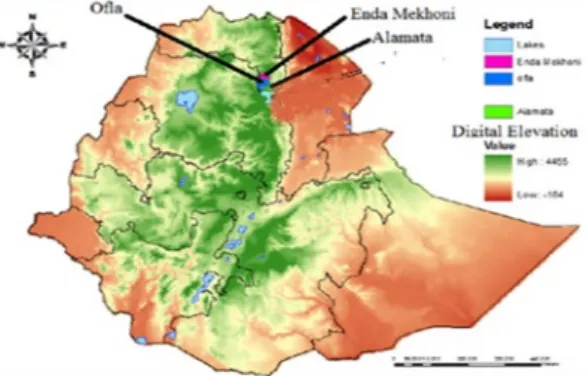
South Tigray Zone is one of the six zones of Tigray Region. The capital town of South Tigray zone, Maychew, is located at a distance of 660 kms north of Addis Ababa and 120 kms south of Mekele, the capital town of the region. The zone is geographically located at 12015’and 13041’ north latitude and 380 59’and 390 54’east longitude, at an altitudinal range of 930 – 3925 masl.
Long term meteorological data indicate that the area receives 400 to 912 mm of mean annual rainfall with mean daily temperature ranges between 9 to 32 ºC. It shares common border with Eastern Tigray zone in the north, Amhara regional state from the south and west, Afar Regional state from the east. According to traditional classification systems, Southern Tigray zone is characterized by three distinct agro-ecologies, including lowlands (locally named as Kolla), midland (Weinadega) and highland (Dega). However, according to the department of Natural Resources Management and Regulatory Department (1998) of Ministry of Agriculture, the zone is classified under the dryland agro-ecologies of tepid to cool sub-moist plains and mountains and plateau (SM2-5). South Tigray is dominated by two major agro-ecologies (lowlands and highlands) and two minor agro-ecologies (mid-altitudes and Peak Mountains). However, the study mainly focused in the two major agro-ecologies (lowlands and highlands) covering a large area of the zone. The zone is mainly characterized by both irrigation based and rain fed based mixed crop-livestock farming systems.
figure 1. Map of the study area
Methods
Data Source and Data Collected, The rainfall data of these stations were collected from National Meteorological Service Agency (NMSA) for duration of 1 hour (1997-2005) extracted from charts and daily rainfall (1970-2009). Predictor data files for SDSM model were downloaded from the Canadian Institute for climate studies (CICS) website (http://www.cics.uvic.ca/scenarios/sdsm/select.cgi).
Building Climate Change Scenarios of Precipitation , General Circulation Model (GCM) Among the different GCM models, the output of only one GCM model was used namely: HadCM3 (Hadley Centre Coupled Model version3). HadCM3 coupled atmosphere-ocean general circulation model is developed at the Hadley Centre in the UK. It is a three-dimensional climate models, composed of two components: the atmospheric model (HadAM3) and the ocean model (HadOM3), which includes a sea ice model. The main reason for the selection of this model for this study is that the model output is available together with the downscaling too. The model result is available for the A2 (medium-high emissions) and B2 (medium-low emission) scenarios. For the two emission scenarios three ensemble members (a, b, and c) are available where each refer to different initial point of climate perturbation along the control run (Hanson et al., 2004 cited in Lijalem, 2006).
Statistical Downscaling Model (SDSM) ,The methodology used in this study followed the procedure previously outlined by Lines and Barrow (Lines et al, 2002). The methodology is fully described in the SDSM ‘Users Manual’, by Wilby and Dawson, (2007), which can be downloaded from the SDSM web site.
Predictor variables selection , The choice of predictor variable(s) is one of the most challenging stages in the development of any statistical downscaling model because the decision largely determines the character of the downscaled scenario. The decision process is also complicated by the fact that the explanatory power of individual predictor variables varies both spatially and temporally (Hessami et al., 2007; Wilby and Dawson, 2007). Observed daily data of large scale predictor variables representing the current climate condition (1961-2001) derived from the NCEP reanalysis data set were used to investigate the percentage of variance explained by each predicatnd-predictor pairs.
Scenario generation , The final step in running SDSM is to use GCM projections to generate future scenarios for the three tri-decadal periods centered on the 2020’s, 2050’s, and 2080’s. In this case twenty ensembles of synthetic daily weather series were produced based on the atmospheric predictor variables derived from HadCM3 GCM model (emission scenarios A2a and B2a) and regression model weights produced during the calibration process
Development of IDF Curves Using Frequency Analysis, The annual maximum rainfall data of the study area were analyzed using the method of frequency analysis and applying mathematical relationships. Gumbel distribution was selected among the probability distributions based on the well-chosen chi-square (
χ
2) test. This test was also used to check the appropriateness of the probability distribution for the respective durations.Results and Discussion
Annual Rainfall Trend and Variability, The result of summary of annual rainfall statistics for this study indicates that the coefficient of variation (CV) , According to Hare (1983) classification, rainfall is considered as less variable, moderately variable, and highly variable when CV is less than 20%, between 20% to 30% and greater than 30%, respectively. Areas with CV>30% are said to be vulnerable to drought, Accordingly, Maichew
is considered less variable stations and Alamata considered moderately variable ,Chercher and mokhoni are considered Highly variable stations. It is the standard deviation of the data set which governs the CV values of the stations as high, medium or low over rainfall variability classification.
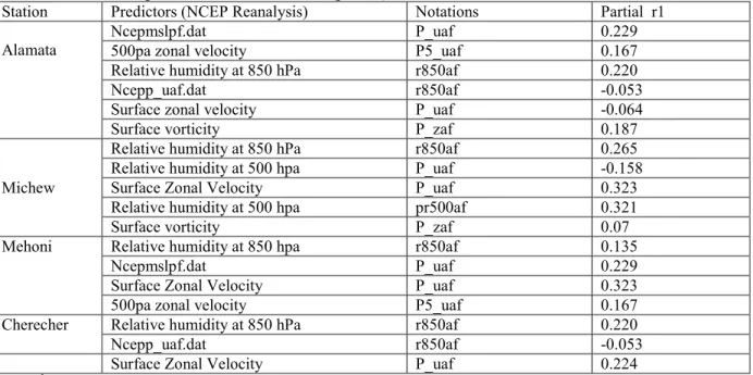
Building Climate Change Scenarios , Selection of Potential Predictor Variable , The first step in the downscaling procedure using SDSM was to establish the empirical relationships between the predictand variables precipitation collected from stations and the predictor variables obtained from the NCEP re-analysis data for the current climate. This was involved in the identification of appropriate predictor variables that have strong correlation with the predictand variable. The next step was the application of these empirical predictor-predictand relationships of the observed climate to downscale ensembles of the same local variables for the future climate. Data supplied by the HadCM3 for the A2 and B2 emission scenarios for the period of 1961–2099 for South Tigray meteorological stations. This is based on the assumption that the predictor-predictand relationships under the current condition remain valid under future climate conditions too. Therefore, according to the above procedure the potential predictors selected for precipitation for the study area were listed in (Table 1).
Table 1 .List of predictor variables that have better spatial and temporal correlation with the predicatnd (rainfall) at two stations with significant level less than 0.05(p<0.05)
Station Predictors (NCEP Reanalysis) Notations Partial r1 Alamata Ncepmslpf.dat 500pa zonal velocity P_uaf P5_uaf 0.229 0.167
Relative humidity at 850 hPa r850af 0.220
Ncepp_uaf.dat r850af -0.053
Surface zonal velocity P_uaf -0.064
Surface vorticity P_zaf 0.187
Michew
Relative humidity at 850 hPa r850af 0.265
Relative humidity at 500 hpa P_uaf -0.158
Surface Zonal Velocity P_uaf 0.323
Relative humidity at 500 hpa pr500af 0.321
Surface vorticity P_zaf 0.07
Mehoni Relative humidity at 850 hpa r850af 0.135
Ncepmslpf.dat P_uaf 0.229
Surface Zonal Velocity P_uaf 0.323
500pa zonal velocity P5_uaf 0.167
Cherecher Relative humidity at 850 hPa r850af 0.220
Ncepp_uaf.dat r850af -0.053
Surface Zonal Velocity P_uaf 0.224
r1
is the partial correlation coefficient(r) shows the explanatory power that is specific to each predictor. All are significant at p = 0.01. hPa is unit of pressure. 1hPa=1mbar=100pa=0.1kpa and af represents African window. The predictor variables were selected based on their partial correlation values and statistical significance level from their counter parts of the 26 reanalysis NCEP predictor variables. These selected predictor variables were then used to create the empirical relationships between the predictand variable (precipitation) collected from stations and the predictor variables obtained from the NCEP re-analysis data for the current climate. That concerned the identification of appropriate predictor variables that have strong correlation with the predictand variable.
Calibrations and Validation , From the thirty-two years of data representing the current climate condition, the first sixteen years (1970-1985) were considered for calibrating the regression models while the remaining sixteen years of data (1986-2001) were used to validate the model for maichew station. But for the other stations (1980-1996) were considered for calibrating and (1997-2014) were used to validate the model. Some of the SDSM setup parameters for event threshold, bias correction and variance inflation were adjusted during calibration to get the good statistical agreement between observed and simulated precipitation. The calibration statistics for predictand variable at Alamata, Maichew Mekhoni and chercher are summarized in Table below.
Table 2. Calibration and validation processes for considered stations
Stations R Square Calibration SE R Square Validation SE
Alamata 0.408 0.276 0.421 0.269
Maichew 0.242 0.417 0.365 0.357
Mehoni 0.354 0.345 0.368 0.415
Cherecher 0.207 0.355 0.335 0.327
According to (Shrestha, Babel et al. 2017), The conditional nature of precipitation which is an intermediate process not only oversee by the given large scale atmospheric predictor variables but also biased by different local conditions such as land use, topography, cloud cover and other associated factors which are not taken in to consideration in the statistical downscaling model (SDSM) due to that the degree of association between the predictand and predictor variables during calibration and validation process looks low down. According to Wilby and Dawson (2007), developers of the SDSM, the explained variances (R2) expected from the predictors are: precipitation values above 10% (0.1) (and in some cases below 10%). Therefore, as shown in Table 2 above , the explained variance (R2) that were found for all the considered stations varies from (0.408, for Alamata and 0.242, for Maichaw for 0.354 Mekhoni and 0.207 for cherecher during calibration); and (0.421, for Alamata and 0.365, for Maichew.0.368 for mekhoni during validation) this result is in line with the recommended one. This result represents there was a good agreement between the predictand and predictor variables and since there is no much difference between calibration and validation statistics in all cases, the model was adopted to be valid for down scaling and generation of the current and future climate forcing scenarios.
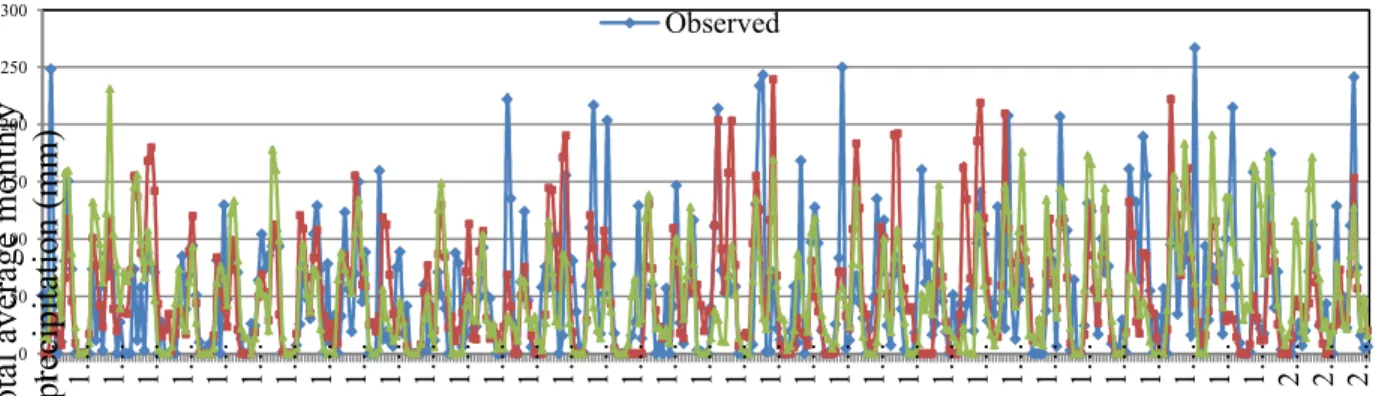
Scenarios Developed for the Base Period (1970-2001), As can be seen in Figure 2. below, SDSM is able to simulate all except the extreme precipitation events at maichew stations. The model underestimates the farthest values in both extremes and keeps more or less an average event. This lack of replicating the extreme values was also observed by Wilby (2005, p.4) and he described it as “the model is less skilful at replicating the frequency of events”. In addition, the total precipitation values were found to be a little bit over and/or underestimated both seasonally andannually
Figure 2. The pattern of monthly precipitation for the base period at Maichew station
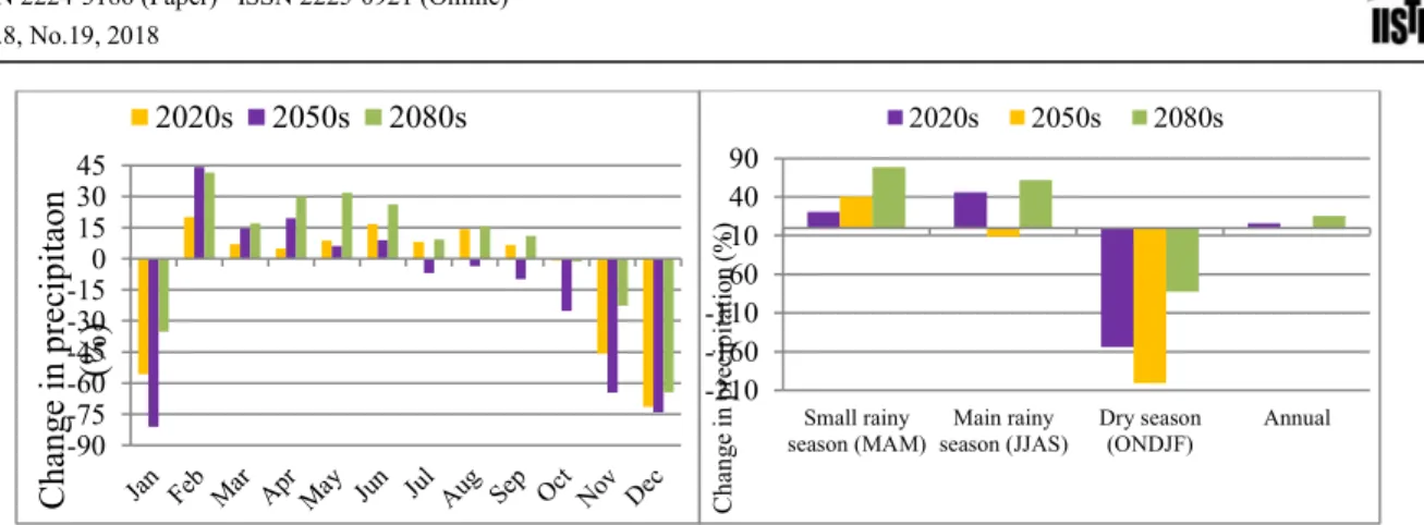
Alamata , According to the precipitation scenarios generated shown in the Figures (3 A) below the average monthly precipitation might show an increase in the months of February, march, April, May, June, July, August and September, but the average monthly precipitation in January, October, November and December might exhibit decrease from the base period level in 2020s for the scenarios. In 2050s, the projected rainfall is expected to increase in months of February, March, April, May, June, July, August, September and October. But the average monthly precipitation is expected to decrease in January, November and December. Moreover, in 2080s the projected rainfall might decrease in months of January, November and December, however, an increase in February, March, May, June, July, August, and September for scenarios. Furthermore, a decrease of 3.01% in month of April and increase of 11.48% in month of October is expected in 2080s scenarios. In seasonal time scale as shown in Figure (3B), the main rainy season (June–September), the rainfall exhibits a relative increase from the baseline period in 2020s (40.25%), 2050s (43.27%) and 2080s (47.01%). In addition, increase in 2020s (19.74%), 2050s (81.03%) and 2080s (9.03%) from the base period for small rainy season (March-May) for the A2 scenario. While in the dry season (October- February) a decrease of 48.15%, 95.89% and 66.99% in 2020s, 2050s and 2080s respectively for the A2 scenario. The mean annual rainfall indicates an increase of 6%, 11%and 8% in 2020s, 2050s and 2080s respectively scenario (Figure 3B).
0 50 100 150 200 250 300 1… 1… 1… 1… 1… 1… 1… 1… 1… 1… 1… 1… 1… 1… 1… 1… 1… 1… 1… 1… 1… 1… 1… 1… 1… 1… 1… 1… 1… 1… 1… 1… 1… 1… 1… 1… 2… 2… 2…
Tot
al
a
ve
ra
ge
m
ont
hl
y
pr
ec
ip
ita
tion (
m
m
)
ObservedFigure 3. A, Change in average monthly precipitation in the future at Alamata B, Average seasonal precipitation for future at Alamata
In 2020s, the projected rainfall is expected to decrease in the months of February, April and October, On the other hand, an increment in January, May, June, July, August and September this scenario from base line period is expected. The projected rainfall is expected to increase in May, July and September, but decrease in January, October and December in 2050s and 2080s respectively from base period. Moreover, an increase and decrease from base period in the months of February, March, April, June, August and November in 2050s and 2080s respectively (Figure 4A). In seasonal time scale, the main rainy season (June–September), the rainfall exhibits a relative increase from the baseline period in 2020s, 2050s, and 2080s for the A2 scenario, while in the small rainy season (March-May) an increase in 2020s and 2050s, and a decrease in 2080s is expected. Moreover, an increase in 2020s and a decrease in 2050s and 2080s is expected during dry season (October-February) for the A2 scenario. The mean annual rainfall indicates an increase of 4.71% and 2.82% in 2020s and 2050s respectively followed by a decrease of 2.81% in 2080s for A2 scenario (Figure 4.B).
Figure 4. (A) Change in average monthly precipitation in the future at Maichew (B) Average seasonal precipitation for future at Maichew
As shown in figure 5A below, In 2050s, the projected rainfall is expected to increase in months of February, March, April, May and June But the average monthly precipitation is expected to decrease in months of January, July, August, September, October, November and December from base period, in 2080s the projected rainfall might decrease in months of January, November and December, however, an increase in February, March, May, June, July, August, and September. In figure 5B, In case of mekhoni , the main rainy season (June–September) rainfall is projected to decrease by 12.12% in 2050s and increase by 46.01% and 61.52% from the baseline period in 2020s and 2080s respectively, whereas in small rainy season (March-May) the rainfall is projected shows an increase of 21.13%, 39.24% and 79.23% in 2020s, 2050s and 2080s respectively. Moreover, the dry season (October- February) rainfall is expected to decrease by 147.89%, 200.68% and 79.90% in 2020s, 2050s and 2080s respectively. The mean annual rainfall is expected to decrease in 2050s by 0.2% and increase by 5.00 % and 15.60% in 2020s and 2080s respectively (Figure 5B).
-60 -50 -40 -30 -20 -100 10 20 30 40 50
C
ha
ng
e i
n
pr
ec
ip
ita
tio
n
(%
)
2020s 2050s 2080s -100 -50 0 50 100 Small rainyseason (MAM) season (JJAS)Main rainy Dry season(ONDJF) Annual
C
ha
ng
e i
n
pr
ec
ip
ita
tio
n
(%
)
2020s 2050s 2080s-30
-20
-10
0
10
20
Ja n Fe b M ar A pr M ay Jun Jul A ug Sep Oct N ov Dec2020s
2050s
2080s
C
cha
ng
e i
n
pr
ec
ip
ita
tion
%
-70 -50 -30 -10 10 30 Small rainy season (MAM) Main rainy season (JJAS) Dry season (ONDJF) Annual 2020S 2050SC
ha
ng
e
in
pr
ec
ip
ita
tio
n
%
figure 5. A Change in average monthly precipitation in the future at Mehoni ( B )Average Seasonal precipitation in the future at Mekhoni
Cherecher , In all future time horizons, there is a decrease in the months of January, February, March, April, May, June, July, August, November and December and increase of September and October is a probable and in 2050s there is decrease in January, October and December and in 2080s a decrease in January, February, April, October, November and December in. However, an increase in months of February, March, May, June, July, August, September and November in 2050s and in 2080s it is also expected to increase in months of May, June, July, August and September from base period figure 6A). The main rainfall season (summer); shows (June–September) rainfall is projected to decrease by 6.74% in 2020s and increase by 21.04% and 13.90% from the baseline period in 2050s and 2080s respectively. Whereas in the small rainy season (March-May)the rainfall is projected to decrease by 6.83% and slight decrease of 0.10% in 2020s and 2080s respectively, but an increase of20.11% in 2050s is expected. Similarly, the dry season (October-February) is expected decrease by 33.78% and 92.59% in 2020s and 2080s respectively; while in 2050s, an increase of 1.96% is expected. Moreover, the mean annual rainfall is expected to decrease in 2020s by 2.3% and increase by 4.74% and 0.014% in 2050s and 2080s respectively from that of base period figure 6B).
figur6 . A Change in average monthly rainfall in the future at Chercher (B) Change in average seasonal rainfall in the future at Chercher
Comparison of Probability Distribution Functions , Selah (2010) developed an empirical formula to estimate design rainfall intensity based on Intensity –Duration -Frequency (IDF) Curves for Riyadh region using the analysis from three different frequency methods namely: Gumbel, Log Pearson III and log Normal. It was concluded that there was no much difference between the result obtained by Gumbel and log Pearson III, while log Normal showed less accuracy. According to Koutsoyiannis, et al., 1998, Gumbel Extreme-Value frequency distribution is the most popular distribution and has received the highest application for estimating large events in various part of the world. For northern Ethiopia, Gumbel's extreme value type I distribution was recommended to fit the annual extreme rainfall data (Cherkos et al., 2006 and Asres, 2008). However, the data series for every station was also tested for Log normal and Log Pearson Type III to check and select the best distribution function. As a result, the Gumbel probability distribution was found to be an appropriate probability distribution function that describe well the given data series for all the considered stations.
-90 -75 -60 -45 -30 -150 15 30 45
C
ha
ng
e i
n
pr
ec
ip
ita
on
(%
)
2020s 2050s 2080s -210 -160 -110 -60 -10 40 90 Small rainyseason (MAM)season (JJAS)Main rainy Dry season(ONDJF) Annual
C ha ng e in p re ci pi ta tio n (% ) 2020s 2050s 2080s -40 -20 0 20 Ja n Fe b M ar A pr M ay Jun Jul A ug Sep Oct N ov Dec C ha ng e in pr ec ip ita tio n (% ) 2020s 2050s 2080s -100-80 -60 -40 -200 20 40 Small rainy season (MAM) Main rainy season (JJAS) Dry season (ONDJF) Annual C ha ng e in pr ec ip ita tio n (% ) 2020s 2050s 2080s
Table 3. Probability Distribution Function
Station of name Type ofDistribution R-square Value for the Indicated Duration (hr)
1 2 3 6 12 24
Mekoni Gumbel EVI 0.921 0.978 0.975 0.972 0.974 0.962 Lognormal 0.923 0.960 0.954 0.954 0.976 0.964 Log Pearson 0.966 0.976 0.964 0.926 0.968 0.969 Chercher EVI 0.979 0.980 0.976 0.970 0.991 0.955 Lognormal 0.933 0.929 0.947 0.960 0.970 0.920 Log Pearson 0.962 0.946 0.968 0.967 0.990 0.960 Maichew EVI 2.879 2.415 1.042 2.042 1.776 2.697 Alamata EVI 2.404 1.710 2.447 0.656 0.767 0.889
IDF curves under climate change for the stations, For the expected changes in rainfall intensities due to climate change, this paper continues to offer the development of future climate IDF curves for un gauged sites. The approach is easier understood when it first be applied to sites with existing IDF curves. The IDF curves were plotted using the predicted values of rainfall intensity using on a double logarithmic scale, using the duration (Td), as abscissa and the intensity (I), as ordinate, with the help of Microsoft office excel 2007. The IDF curves plotted for the stations under climate change are presented in following Figures 7 abd 8 . The plots should serve to meet the need for rainfall IDF relationships in the study area for return periods of 2 to 100 years under climate change condition.
figure 7 A IDF curves for Mehkoni station 2050's B IDF curves for Chercher station for 2050's
Figure 8 A IDF curves for Alamata station for 2050's B, IDF curves for Maichew station for 2050's
Comparison of IDF results, Comparison of IDF results was made between IDF curve developed under climate change scenarios with the historic rainfall (IDF) relationships for stations as well. Relative difference between the curves is determined using the following relationship (Prodanovic and Simonovic, 2008 and Solaiman and Simonovic, 2011as
The model estimations show different results, with the extreme rainfall. In 2050s, climate change shows slight decrease and increase in rainfall intensity than the existing rainfall intensity for all durations(1, 2,3, 6, 12 and 24 hours) and return periods at chercher Figure 9A. Results of the comparison between historic rainfall and climate change rainfall intensity data set for specified return periods indicate that, the rainfall magnitude might decrease for all duration (1, 2,3, 6, 12 and 24 hours). in Figures 9B below at Mehkoni station
1 10 100 1 10 100 2 Years 5 Years 10 Years 25 Years 50 Years 100 Years Rainfall Duration ( hr
)
R
ai
nf
al
l i
nt
ens
ity
(m
m
/hr
)
1 10 100 1 10 100 2 Years 5 Years 10 Years 25 Years 50 YearsDuration ( hr)
R
ai
nf
al
l i
nt
ens
ity
m
m
/hr
1 10 100 1 10 100 2 Years 5 Years 10 Years 25 Years 50 Years 100 Years Rainfall Duration (hr)R
ai
nf
al
l i
nt
ens
ity
in
m
m
/hr
1 10 100 1 10 100 2 Years 5 Years 10 Years 25 Years 50 Years 100 Years Ranfall Duration( hr) R ai nf al li nt ens ity ( m m /hr)
D i fferen ce = Ħx1- x2Ħ Ħx1 + x2Ħ 2 × 10 0figure 9. A chercher B, Mehkoni
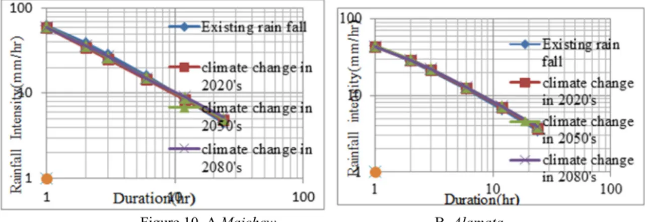
The relative results indicate that difference between rainfall intensities (percentage) of climate change scenario and historic rainfall in all cases of the study area. By 2050s climate time line, the intensity of rainfall shows an increasing trend for (2, 3, 6 and12hrs) duration , while there will be a decrease for the shorter (1hr) duration and longer (24hr) duration almost for all return periods. Besides, the rainfall intensity by 2050s will be increase without failure throughout the given durations and return periods with a slight decrease for the 24hr duration .as shown in figures 10 A&B below in Maichew and Alamata .
Figure 10. A Maichew B Alamata
Generally to compare the IDF results between historic rainfall and climate change rainfall intensity data set, it is difficult to say whether it is decreasing or increasing for the future time. The weakness of this study and the historic studies may also be one of the reasons this based on observation errors: frequently, external factors influence an observation, such as temperature and air pressure variations during observation model or system errors. And also the model (SDSM) is less skillful at replicating the frequency of events. There is also general truth that the severity to prediction nature especially rainfall: it is conditional process because of its dependence on other intermediate processes like the occurrences of humidity, cloud cover, and/or wet-days. But this is prediction or forecasts for a future event in the sense of aiming at the truth. Because of the natural uncertainties, the newly developed IDF curves are unable to provide an accurate estimate of future extreme rainfall, but they establish a significant fact: the future climate will not be the same as the historic one. That rainfall magnitude will be different in the future,(Predrag Prodanovic and Slobodan P. Simonovic 2007)
Conclusions and Recommendations
the impact of climate change on IDF curves at the study areas were carried out to address part of the global problem. The future climate change scenarios were generated by using SDSM model to generate synthetic hourly data and to simulate the impacts of climate changes on the IDF curves of the study areas. Finally, adaptation measures that can serve to reduce the damages were proposed. The study confirmed that the Statistical DownScaling Model (SDSM) is able to simulate all except the extreme climatic events. The model underestimates the farthest values in both extremes and keeps more or less an average event. Nevertheless, the simulated climatic variables generally follow the same trend with the observed one. SDSM more accurately reproduced monthly and seasonal climatic variables averaged over years than individual monthly and seasonal values in a single year at the stations. Development of IDF curves is critical for undertaking short-term measures as well as long-term running and versions in water related sectors. This study provides a solution to obtain present climate IDF curves for un gauged sites outside the domain of gauged stations in the study area. The anticipated impacts of climate change especially increase in rainfall intensity and its frequency appreciates the derivation of future IDF curves in this study. Studies, which focus on likely future climate change scenarios and
1 10 100 1 10 100 Existing rain fall climate change in 2020's climate change in 2050's climate change in 2080's Duration(hr
)
R
ai
nf
al
l I
nt
ens
ity
(
m
m
/hr
)
1 10 100 1 10 100 Existing rain fall climate change in 2020's climate change in 2050'sDuration (hr)
R
ai
nf
al
l i
nt
ens
ity
(m
m
/hr
)
information for planning, designing and evaluation of water resource systems, drainage works etc. The IDF relationships enable estimation of intensity of rainfall corresponding to any required rainfall duration and frequency.
The current IDF curves should be revised to reflect the potential impact of climate change
Results of any impact studies are highly dependent on the quality of input data. Therefore, increasing the number of meteorological and hydrological stations is very important
For the use of any models input data should be checked for missing and unrealistic values in order get accurate results
The GCM outputs, the emission scenarios and the downscaling methods used for this study have certain level of uncertainty. Therefore, further study should reduce the uncertainty by using additional GCMs, downscaling methods and emission scenarios
New infrastructure should be designed on the basis of historical information on changes in extremes and projected future changes
There should be regular updating of Intensity-Duration-Frequency curves for all major zone to take into account the effect of climate change.
REFERENCES
Asres Geda. 2008. Development and Regionalization of Intensity Duration Frequency (IDF) Relationships for Amhara and Tigray Regions. MSc. Thesis.AdisAbaba University, Adis Ababa, Ethiopia
Barnett, T.P.; Pierce, D.W.; Hidalgo, H.G.; Bonfils, C. B.; Santer, D.; Das, T.; Bala, G.; Wood, A.W; Nozawa, T.; Mirin, A.A.; Cayan, D.R.; and Dettinger, M.D. 2008. Human-induced changes in the hydrology of the Western United States, Science, 319, 1080–1083, DOI:10.1126/science.1152538.
Cherkos Tefea, Muluneh Yitayel and Yilma Seleshi. 2006. Rainfall Intensity-Duration Frequency Relationship for Northern Ethiopia. Journal of Ethiopian Engineers and Architects, Adis Ababa, Etiopia. VoL 23, 29-38.
Cherkos Tefea, Muluneh Yitayel and Yilma Seleshi. 2006. Rainfall Intensity-Duration Frequency Relationship for Northern Ethiopia. Journal of Ethiopian Engineers and Architects, Adis Ababa, Etiopia. VoL 23, 29-38. Hegerl, G.C.; Zwiers, F.; Stott, P.; and Kharin, S. 2004: Detectability of anthropogenic changes in annual
temperature and precipitation extremes. Journal of Climate, 17, 3683–3700.
IPCC (Intergovernmental Panel on Climate Change), Climate change 2007. Impacts, adaptation and vulnerability, in Parry, M.L., Canziani, O.F., Palutikof, J.P., van der Linden, P.J., and Hanson, C.E., eds., Contribution of Working Group II to the Fourth Assessment Report of the Intergovernmental Panel on Climate Change: Cambridge, United Kingdom, Cambridge University Press.
Kharin, V.V.; Zwiers, F.W.; Zhang, X.; and Hegerl, G.C. 2007. Changes in temperature and precipitation extremes in the IPCC ensemble of global coupled model simulations. Journal of Climate, 20, 1419-1444, DOI: 10.1175/JCLI4066.1
Kim, T., Shin J., Kim K., and Hoe J, (2008), “Improving Accuracy of IDF curves using long and short duration separation and multi-objective Genetic algorithm ‘’, World Environmental and water resources Congress 2008 Ahupua’s, ASCE.
Koutsoyiannis, D. Kozonis and A Manetas. 1998. A Mathematical Framework for Studying Rainfall Intensity-Duration- Frequency Relationships. Journal of Hydrology, 206, II R - 135 Athens.
Liew SC, VRaghavan S, Liong S-Y (2013) How to construct future IDF curves, under changing climate, for sites with scarce rainfall records? Hydrol Process. 28(8):3276–3287.
Lijalem, Z. A. 2006. Climate Change Impact on Lake Ziway Watershed Water Availability,Ethiopia, University of Applied Sciences Cologne,Germany
Lines, G.S., Barrow, E.M., 2002. Regional Climate Change Scenarios in Atlantic Canada Utilizing Downscaling Techniques: Preliminary Results. AMS Preprint, 13-17 January 2002, Orlando FL,USA.
Mailhot, A. and Duchesne, S. 2010. Design criteria of urban drainage infrastructures under climate change. Water Resource Plan Management 136:201–208.
McCuen R (1998) Hydrologic analysis and design. Prentice-Hall, Englewood Cliffs, NJ.
Mehdi, B., C. Mrena and A. Douglas, 2006. Adapting to climate change: An introduction for Canadian Municipalities. Canadian Climate Impacts and Adaptation Research Network (C-CIARN).
Milly, P.C.D.; Betancourt, J. M.; Falkenmark, Hirsch, R.M.; Kundzewicz, Z.W.; Lettenmaier, D.P.; and Stouffer, R.J. 2008: Stationarity is dead: whither water management? Science, 319, 573–574.
Min, S.-K.; Zhang, X.; and Zwiers, F. 2008. Human-induced Arctic moistening. Science, 320, 518–520, DOI:10.1126/science.1153468.
Nash, J. E. and Sutcliffe, J. V. 1970. River flow forecasting through conceptual models, Part A: discussion of principles. J Hydrol;10:282–290.
Precipitation in the Monsoon Area of Vietnam. Graduate School of Urban and Environment Engineering, Kyoto University, 49: 93-103
NMA (2007). National Adaptation Programme of Action of Ethiopia (NAPA). Final draft report. National Meteorological Agency, Addis Ababa.
NMSA (National Meteorological Service Agency), 1996. Assessment of Drought in Ethiopia. No.2. Addis Ababa, Ethiopia.
NMSA (National Meteorological Services Agency), 2001. Initial National Communication of Ethiopia to the UNFCCC. Addis Ababa, Ethiopia.
Predrag Prodanovic and Slobodan P. Simonovic, 2007. Development of rainfall intensity duration frequency curves for the City of London under the changing climate. Water Resources Research Report no. 058, Facility for Intelligent Decision Support, Department of Civil and Environmental Engineering. London, Ontario, Canada.
Prodanovic P, Simonovic SP (2007) Development of rainfall intensity duration frequency curves for the City of London under the changing climate. Water Resour Res Report, London.
Prodanovic, P. and Simonovic, S.P. 2008. Intensity-Duration-Frequency under Changing Climatic Conditions. 4th International Symposium on Flood Defense: Managing Flood Risk, Reliability and Vulnerability, Toronto, Ontario, Canada.
Selah, A. A., (2010), Developing an Empirical Formulae to estimate rainfall intensity in Riyadh region. Journal of king Saud University-Engineering Sciences .www.sciencedirect.com’
Soil and Water Conservation Society (SWCS) (2003), Conservation implications of climate change: Soil erosion and runoff from cropland, report, Ankeny, Iowa.
Wilby, R. L. 2005. A framework for assessing uncertainties in climate change impacts: Low-flow scenarios for the River Thames, UK. WATER RESOURCES RESEARCH,
Wilby, R. L. and Dawson, C. W. 2007. SDSM 4.2 — A decision support tool for the assessment of regional climate change impacts, User Manual.
Wolcott SB, Mroz M, Basile J (2009) Application of Northeast Regional ClimateCenterResearch results for the purpose of evaluating and updating Intensity-Duration-Frequency (IDF) Curves.CaseStudy: Rochester, New York. In: Proceedings of world environmental andwater resou rces congress 2009. Kansas City, Missouri. Wright P, DeGeatano A, Merkel W, Metcalf L, D. Quan Q, Zarrow D (2010) Updating rainfall intensity duration
curves in the Northeast for runoff prediction. In: Proceedings of ASABE annual international meeting. Pittsburgh, Pennsylvania
Zhang, X.; Zwiers, F.W.; Hegerl, G.C.; Lambert, F.H.; Gillett, N.P.; Solomon, S.; Stott, P.A.; and Nozawa, T. 2007. Detection of human influence on twentieth-century precipitation trends. Nature, DOI:10.1038/nature06025.