atmosphere
ArticleObserved Response of the Raindrop Size Distribution
to Changes in the Melting Layer
Patrick N. Gatlin1,*ID, Walter A. Petersen1ID, Kevin R. Knupp2and Lawrence D. Carey2 1 NASA Marshall Space Flight Center, Huntsville, AL 35805, USA; [email protected]
2 Department of Atmospheric Science, University of Alabama in Huntsville, Huntsville, AL 35805, USA; [email protected] (K.R.K.); [email protected] (L.D.C.)
* Correspondence: [email protected]; Tel.: +1-256-961-7910
Received: 15 July 2018; Accepted: 10 August 2018; Published: 18 August 2018
Abstract:Vertical variability in the raindrop size distribution (RSD) can disrupt the basic assumption of a constant rain profile that is customarily parameterized in radar-based quantitative precipitation estimation (QPE) techniques. This study investigates the utility of melting layer (ML) characteristics to help prescribe the RSD, in particular the mass-weighted mean diameter (Dm), of stratiform rainfall. We utilize ground-based polarimetric radar to map the ML and compare it withDmobservations from the ground upwards to the bottom of the ML. The results show definitive proof that a thickening, and to a lesser extent a lowering, of the ML causes an increase in raindrop diameter below the ML that extends to the surface. The connection between rainfall at the ground and the overlying microphysics in the column provide a means for improving radar QPE at far distances from a ground-based radar or close to the ground where satellite-based radar rainfall retrievals can be ill-defined.
Keywords:microphysics; radar; precipitation
1. Introduction
Radar-based measurements of rainfall are vital to understanding the distribution of precipitation over large watersheds. Even though dual-polarimetric radar technology and the associated parameters measured enable improved rainfall estimation compared to traditional (i.e., single-polarization) radar [1–3], dual-polarimetric radars still suffer from many of the same sampling uncertainties associated with accurately estimating rainfall at distant ranges from the radar. For example, regardless of polarization characteristics, beam broadening causes the spatial resolution of radar measurements to degrade with increasing range [4], enabling non-uniform beam filling to impact the accuracy of radar-based estimates of rainfall [5,6]. Ground-based weather radars obtain measurements at increasingly higher heights as the radar beam travels away from the radar due to Earth curvature and gradients in the refractive index driven by vertical gradients of atmospheric temperature and humidity. Thus, radar derived rainfall maps may not be representative of the actual rainfall totals observed at the ground, especially at great distances from the radar (e.g., during winter a typical 1◦wide radar beam scanned at an elevation angle of 0.5◦may encounter melting precipitation around 100 km from the radar) and in regions of complex terrain that can inhibit use of measurements obtained at the lowest elevation angles.
It is customary in radar-based quantitative precipitation estimation (QPE) to assume a constant rainfall profile below the lowest altitude of a given radar measurement or to apply a correction based on some model of the vertical profile of reflectivity (VPR), for example, References [7,8], but vertical variability in the raindrop size distribution (RSD) can disrupt these methods by undermining the basic assumption of a constant rain profile. Satellite-based retrieval techniques can also be greatly impacted by RSD variability since due to main beam clutter they must use measurements that are typically no Atmosphere2018,9, 319; doi:10.3390/atmos9080319 www.mdpi.com/journal/atmosphere
Atmosphere2018,9, 319 2 of 18
lower than 500–1000 m above the ground at nadir points [9]. Moreover, satellite-based radar estimates of rainfall made at higher microwave frequencies can be greatly affected by attenuation [10,11]. Although numerous other factors contribute to the sampling uncertainties (e.g., instrument calibration, sampling strategy, etc.), some of which are rather complex [1,5], all else being equal it ultimately is our ability to fully describe the vertical column of precipitation and its variability using radar measurements (ground, airborne or space-based) that determines the accuracy of radar QPE.
This study addresses radar-based QPE, and more specifically, the range-dependent errors by examining the physical origin of the RSD as well as the factors that influence its size evolution. Raindrops often develop from the melting of precipitation-sized ice hydrometeors [12]. For example, melting snowflakes are a common source of rainwater in stratiform precipitation. Thus, characteristics of the melting layer (ML) prescribe the initial state of the RSD, and as such, measurements of the ML may provide additional information beneficial to radar QPE. Accordingly, we hypothesize that a relatively thick ML (and/or low ML) produced by stratiform precipitation results in larger raindrops. Several studies have found that larger raindrops were observed at the ground beneath more intense radar reflectivity bright bands [13–16]. An example of this existing conceptual model using vertical profiles of reflectivity is shown in Figure1. Thicker (or deeper) portions of the bright band in equivalent radar reflectivity factor are seemingly connected via precipitation fallstreaks to a temperature zone favorable for dendritic growth [12,17], which is seemingly enhanced in the presence of weak convective motions. Below these thicker regions of the bright band, enhanced reflectivity (Z) is often present at low-levels (<1–2 km), indicative of larger raindrops (Z is proportional to sixth power of the diameter) emanating from a thicker (or deeper) melting layer. However, the reflectivity bright band is a radar measurement-based manifestation of the ML and can only be used to indirectly describe rainfall intensity.
impacted by RSD variability since due to main beam clutter they must use measurements that are typically no lower than 500–1000 m above the ground at nadir points [9]. Moreover, satellite-based radar estimates of rainfall made at higher microwave frequencies can be greatly affected by attenuation [10,11]. Although numerous other factors contribute to the sampling uncertainties (e.g., instrument calibration, sampling strategy, etc.), some of which are rather complex [1,5], all else being equal it ultimately is our ability to fully describe the vertical column of precipitation and its variability using radar measurements (ground, airborne or space-based) that determines the accuracy of radar QPE.
This study addresses radar-based QPE, and more specifically, the range-dependent errors by examining the physical origin of the RSD as well as the factors that influence its size evolution. Raindrops often develop from the melting of precipitation-sized ice hydrometeors [12]. For example, melting snowflakes are a common source of rainwater in stratiform precipitation. Thus, characteristics of the melting layer (ML) prescribe the initial state of the RSD, and as such, measurements of the ML may provide additional information beneficial to radar QPE. Accordingly, we hypothesize that a relatively thick ML (and/or low ML) produced by stratiform precipitation results in larger raindrops. Several studies have found that larger raindrops were observed at the ground beneath more intense radar reflectivity bright bands [13–16]. An example of this existing conceptual model using vertical profiles of reflectivity is shown in Figure 1. Thicker (or deeper) portions of the bright band in equivalent radar reflectivity factor are seemingly connected via precipitation fallstreaks to a temperature zone favorable for dendritic growth [12,17], which is seemingly enhanced in the presence of weak convective motions. Below these thicker regions of the bright band, enhanced reflectivity (Z) is often present at low-levels (<1–2 km), indicative of larger raindrops (Z is proportional to sixth power of the diameter) emanating from a thicker (or deeper) melting layer. However, the reflectivity bright band is a radar measurement-based manifestation of the ML and can only be used to indirectly describe rainfall intensity.
Figure 1. A time-series of equivalent radar reflectivity above radar level (ARL) from the University of Alabama in Huntsville (UAH) X-band vertically pointing radar (XPR) measurements of a stratiform precipitation event in Huntsville, Alabama. Time is given in Universal Coordinated Time (UTC). In general, there is a lack of quantitative evidence more directly relating microphysical properties of the ML to the RSD and its evolution. Although several studies have noted relatively little variability in the vertical evolution of the RSD within stratiform precipitation, the reference for comparison is often to the RSD evolution in convective precipitation, for example, References [18– 20]. Very little has been done to examine differences in vertical RSD evolution within stratiform precipitation for different ML characteristics. Such an investigation is vital to developing procedures that employ ML characteristics (or its radar manifestations) to improve radar rainfall estimation. In
Figure 1.A time-series of equivalent radar reflectivity above radar level (ARL) from the University of Alabama in Huntsville (UAH) X-band vertically pointing radar (XPR) measurements of a stratiform precipitation event in Huntsville, Alabama. Time is given in Universal Coordinated Time (UTC).
In general, there is a lack of quantitative evidence more directly relating microphysical properties of the ML to the RSD and its evolution. Although several studies have noted relatively little variability in the vertical evolution of the RSD within stratiform precipitation, the reference for comparison is often to the RSD evolution in convective precipitation, for example, References [18–20]. Very little has been done to examine differences in vertical RSD evolution within stratiform precipitation for different ML characteristics. Such an investigation is vital to developing procedures that employ ML
characteristics (or its radar manifestations) to improve radar rainfall estimation. In this study, we use high resolution polarimetric radar scanning strategies of the rain column and ML accompanied by nearby disdrometers at the ground to examine the mass-weighted mean diameter (Dm) response to
changes in the ML geometry (i.e., thickness and height above ground).
The radars and disdrometers used for this study as well as techniques for connecting the ML to the Dmare described in Section2. Results of theDmresponse at the ground and in the vertical to changes in the ML are given in Section3. These findings are discussed in Section4as they relate to those from past ML and microphysical studies. The final section provides a summary of the findings and proposes avenues to further explore.
2. Datasets and Methods 2.1. Instrumentation and Datasets
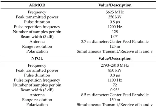
Over 90% of the radar data examined in this study were obtained with the Advanced Radar for Meteorological and Operational Research (ARMOR) located in Huntsville, Alabama and jointly owned and operated by the University of Alabama in Huntsville (UAH) and WHNT-TV, which is a local television station in Huntsville. The ARMOR is a polarimetric Doppler radar that operates in the C-band frequency range [21]. Data collected with NASA’s dual-polarimetric S-band radar (NPOL) [22], during the NASA Global Precipitation Measurement (GPM) Mission Iowa Flood Studies (IFloodS) campaign, which took place in eastern Iowa during the spring of 2013 [23], are also used to examine changes in the ML. Both ARMOR and NPOL transmit using slant±45◦linear polarization [24,25]. Descriptions of both radars and their configurations for the datasets used in this study are provided in Table1.
Table 1.Characteristics of the Advanced Radar for Meteorological and Operational Research (ARMOR) and NASA’s dual-polarimetric S-band (NPOL) radars used in this study.
ARMOR Value/Description
Frequency 5625 MHz
Peak transmitted power 350 kW
Pulse duration 0.8µs
Pulse repetition frequency 1200 Hz
Number of samples per bin 128
Beam width (3 dB) 1.07◦
Antenna 3.7 m diameter; Center Feed Parabolic
Range resolution 125 m
Polarization Simultaneous Transmit/Receive of h and v
NPOL Value/Description
Frequency 2790–2810 MHz
Peak transmitted power 850 kW
Pulse duration 0.8µs
Pulse repetition frequency 1100 Hz
Number of samples per bin 72
Beam width (3 dB) 0.95◦
Antenna 8.5 m diameter; Center Feed Parabolic
Range resolution 150 m
Polarization Simultaneous Transmit/Receive of h and v
Retrieval of vertical profiles of Dmfrom ARMOR and NPOL are obtained at distance of 15 km
from range-height indicator (RHI) scans that were repeated at an interval of 1–2 min. These distances are selected due to the presence of in-situ disdrometer measurement of raindrops at the ground along those radar azimuths. Each RHI scan consists of 0.1–0.2◦spacing between elevation angles to oversample the vertical dimension. This scanning strategy allows theDmprofiles to be obtained with
a high degree of vertical resolution as well as a relatively high degree of temporal resolution. As a result, although the beam is around 250 m wide at 15 km range, the elevation sampling resolution (i.e., effective “vertical” resolution) is roughly 50 m due to the 0.1–0.2◦spacing employed.
Two-dimensional video disdrometers (2DVD) are used to obtain RSD measurements at the ground and serve as the basis for the radar scattering simulations we use to retrieve the verticalDm profile. The 2DVD is an optical disdrometer that uses two line-scan cameras to provide orthogonal measurements of raindrop size and shape [26]. The fields of view overlap to form an approximately 10 cm×10 cm measurement area with a resolution of 0.2 mm. Since the field of view of each camera is vertically offset by 6–7 mm, which was monitored via routine calibration [26], the raindrop fall velocity can also be directly measured.
Most of our ground-based RSD measurements were recorded in Huntsville, Alabama and largely obtained with the low-profile version of the 2DVD owned by Colorado State University (CSU) and occasionally complemented (intermittent due to field campaign use) with several compact 2DVD versions owned by the NASA GPM Ground Validation (GV) program. Both versions of the 2DVD are similar in height and resolution but the compact version is the newer generation that has a slightly smaller footprint and updated electronics [27]. In Huntsville, the 2DVDs were deployed within a 10 m×10 m area at the National Space Science and Technology Center (NSSTC) on the UAH campus approximately 15 km east-northeast of the ARMOR radar. The remaining 19% of the RSD measurements we also use are from the six GPM GV compact 2DVDs deployed along a line extending southeast of NPOL in east-central Iowa during the GPM IFloodS campaign. A summary of these 2DVD measurements is given in TableA1. We used over 134,000 min of rainfall from multiple 2DVDs to perform the radar scattering simulations discussed in Section2.3., but to compare the ground-based raindrop size measurements with the radar-inferred ML characteristics we only use one disdrometer at each location—in Huntsville we use CSU’s low-profile 2DVD at 15 km east-northeast ARMOR and in Iowa we use GPM GV’s compact 2DVD (SN35) at 15 km southeast of NPOL. This much smaller subset, which consists of only 2261 min, is largely a result of the corresponding times that RHI scans were conducted over the disdrometers during stratiform precipitation and a ML was identified from the radar measurements.
2.2. Radar Identification of the Melting Layer
A primary objective of this study is to define the characteristics and evolution of the raindrop size below the ML and as a function ML properties and therefore we must first locate the ML boundaries in a given radar volume. It is not the purpose of this study to introduce a new ML detection algorithm for radar. Many other studies have already devised ML detection algorithms using dual-polarimetric radar measurements [28–32]. Accordingly, we follow these previous studies and identify the ML by considering the dual-polarimetric measurement of co-polar correlation coefficient (ρhv), which for rain and dry snow is typically very near unity but decreases to values below 0.98 within mixed-phase precipitation [33,34].
To map out the ML we searched for layers ofρhv< 0.98 situated near the 0◦C level as estimated from nearby Rapid Update Cycle model analysis [35] and within 500 m of the reflectivity bright band maximum. These latter two constraints help mitigate false ML detections in regions of clutter or low signal to noise ratio whereρhvcan be significantly reduced. The top and bottom of theρhv< 0.98 layer are then defined as the ML top and ML bottom, respectively. When using the ARMOR radar data, we further refine the height of the ML bottom by raising it to account for the possibility ofρhv≤0.94 at C-band radar frequencies due to large raindrops [36,37], which can be present immediately below the ML. The ML bottom is also used to consider impacts of ML proximity to ground on the RSD.
Although algorithm development for ML identification is not the focus of this study, selection of the ML boundaries does play a key role and thus it is necessary to determine the uncertainty in the estimates of ML bottom and thickness (or depth) since beam broadening and non-uniform beam filling can falsely enhance the ML depth estimated at 15 km from the radar [4]. We compare the ML from
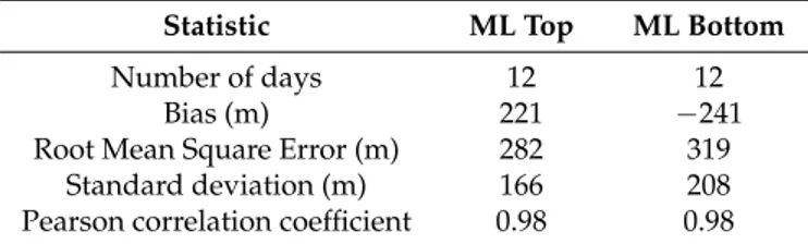
ARMOR RHI scans with UAH X-band Profiling Doppler radar (XPR) measurements during twelve precipitation events over the NSSTC. The XPR is located 15 km from ARMOR and also co-located with some of the disdrometers used in this study. The vertical-pointing measurements collected by the XPR during these twelve events provide an excellent signature of hydrometeor melting at a vertical resolution of 50 m. Following the approach of [38], we define the boundaries of the XPR-detected ML using the curvature of the Doppler velocity measured above and below the peak of the radar bright band. The statistics of the ML comparison for the twelve events are given in Table2. The ARMOR estimated ML top is an average of 221 m higher than from the XPR and the ARMOR estimated ML bottom is an average of 241 m lower than the XPR estimate. These statistics are consistent with the performance of other dual-polarimetric ML identification algorithms [29,31,39]. Assuming that the XPR Doppler velocity profiles represent “truth”, we adjusted the ML boundaries estimated from dual-polarimetric RHI scans at 15 km range for their respective biases and then use the bias-corrected data in subsequent comparisons for examining RSD characteristics.
Table 2.Performance of melting layer (ML) identification from ARMOR range-height indicator (RHI) scans relative to the University of Alabama in Huntsville X-band Doppler Profiling Radar (XPR) estimates of the ML.
Statistic ML Top ML Bottom
Number of days 12 12
Bias (m) 221 −241
Root Mean Square Error (m) 282 319 Standard deviation (m) 166 208 Pearson correlation coefficient 0.98 0.98
Also, when estimating the ML characteristics from each RHI scan, we account for precipitation trails, or fall streaks, present below the radar bright band that can have adverse impact on the microphysical interpretation of radar data [40–43]. We manually follow the precipitation trails upward from the location of the disdrometer to its source region above the ML. This enables the RSD measurements at the ground and those retrieved from the radar RHI scans to be physically connected to where they originated near the ML.
2.3. Retrieval of the Raindrop Size Distribution
The 2DVD measurements are filtered using environmental temperature, particle fall speed and shape to mitigate contamination of the one minute (1-min) RSD spectra by non-rain particles (e.g., hail, snow, calibration spheres) following the technique of [44]. The resultant 1-min RSD spectra are described using a normalized gamma RSD model [45,46],
N(D) =NwFµ(D/Dm), (1)
which consists of three parameters—Nw, the normalized intercept parameter,Dm, the mass-weighted mean diameter, andµ, a shape parameter that is contained within the probability density function
(PDF) given byFµ(D/Dm) following the nomenclature used by Reference [45]. We follow the approach
used by Reference [47] to computeDmandNwfrom the measured 1-min RSD spectra and minimize the difference between the measuredN(D)and that given by the gamma RSD in (1) to find the optimal value ofµ. Since we are interested in the evolution of the raindrop size, we focus onDm, which is defined as the ratio of the fourth and third moments of the measuredN(D), in our analysis of the RSD. In order to retrieve Dm from the radar RHI scans, we use the 1-min gamma RSD characteristics—Nw,Dmandµ—obtained from the 2DVDs and nearby temperature measurements
(10 m away from the 2DVDs in Huntsville and about 20-km from 2DVDs in Iowa) to perform numerical scattering simulations via the commonly used T-matrix/Mueller matrix methodology [48–51] based
on the extended boundary condition method [52,53]. Although [54,55] already found empirical relationships forDmat C-band using about 7500 min of the Huntsville, Alabama dataset, they fit the data to the median volume diameter (D0), which is slightly different from Dm. Furthermore, we use a
much larger dataset in this study (TableA1). Details on our radar scattering simulations and derivation of the empirically determined equations for retrievingDmfrom the radar are given in the AppendixA. The overall uncertainties (mean standard error) in the ARMOR and NPOL estimates ofDmare 8% and 12%, respectively, and are greatest forDm< 1 mm and less than 6–8% for 1.2 mm <Dm< 2.4 mm consistent with other radar retrievals of RSD at S-band and C-band [55–58].
Radar measurements collected during RHI scans over the disdrometers are used with Equations (A1) and (A2) to retrieve the Dm profile (i.e., from the ground to the bottom of the ML). Next the radar samples obtained at each height are averaged over a 3 km horizontal distance centered on the slanted precipitation trail to reduce large gate-gate (i.e., small-scale) fluctuations in the measured ZDR, which can be noisy at C-band [58–60]. Here we implicitly assume that the precipitation
characteristics are homogenous over a 3 km distance, which is a reasonable assumption for stratiform rainfall, especially for radar retrievals of the characteristic raindrop diameter that can exhibit a spatial correlation exceeding 0.8 at distances of 3- to 30-km [61,62].
3. Results
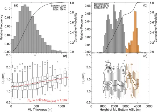
Over 2200 min of radar RHI scans and 2DVD measurements are examined to estimate the ML and RSD characteristics during 36 days of stratiform precipitation observed in Huntsville, Alabama and the IFloodS ground site (2DVD SN35) that was 15 km southeast of NPOL in east-central Iowa. These cases consist of widespread stratiform events produced by mesoscale convective complexes (MCCs), synoptic scale lift (e.g., warm front) and two tropical systems. About 81% of the MLs diagnosed using the RHI scans are 100 m to 600 m thick (Figure2a). The wide and multi-modal distribution of ML heights found in Figure2b reflects changes in the seasonal temperature profile and meteorological regime. Nearly 75% of ML bottoms are 1000 m to 2800 m above ground level (AGL) and roughly 20% were obtained during the remnants of two tropical cyclones that had ML bottoms between 3500 m and 4000 m AGL. The mean ML thickness estimated from polarimetric RHI scans and adjusted for biases (Table2) is 352 m with a standard deviation of 196 m, which is comparable to that inferred from aircraft-based particle images through the ML [63,64]. The equivalent radar reflectivity bright band is also mapped [65] to examine its ability to represent the ML boundaries relative to the dual-polarimetric approach. The top of the bright band in these stratiform events is an average of 100 m higher than that of theρhv-based estimate of ML top and the bottom of the bright band is 80 m lower than that of theρhv-based estimate of ML bottom. The average bright band thickness was around 500–550 m, similar to that found by Reference [65].
3.1. Raindrop Sizes at the Ground
The raindrop sizes measured at the ground with 2DVDs located about 15 km away from the radars are also plotted in Figure2. Figure2c suggests an increasing trend inDm(i.e., raindrop size) at the ground with increasing ML thickness, especially for the more frequently observed ML thicknesses (150–750 m). We find a decreasing trend ofDmwith ML bottom, but theDmtrend does not exhibit an overall decrease across the entire range of estimated ML bottom heights (Figure2d). For example, those ML bottoms at altitudes exceeding 3500 m AGL are associated with greaterDmthan the ML bottoms below 1500 m AGL. However, the multi-modal distribution of the ML heights somewhat masks the decrease ofDmwith increasing ML height. Considering only theDmmeasured at the ground when ML heights exhibit a more normal distribution (e.g., the group of bins between 3000 and 4200 m highlighted in Figure2b), as the height of the ML bottom ascended 1000 m, the meanDmgenerally decreased from 1.7 mm to 1.2 mm (Figure2b,c). Similar, but less pronounced, trends occurred beneath other subsets of MLs at lower heights (e.g., ML bottoms between 2000 and 2400 m AGL in Figure2d).
Although Figure2c clearly indicatesDmincreases with increasing ML thickness, we perform an analysis of variance (ANOVA) to test the null hypothesis—Dmdoes not vary with ML thickness—and find that it can be rejected with a 99% confidence level. HenceDmvaries with ML thickness. We find a strong linear relationship exists between ML thickness andDm(Pearson correlation coefficient, r, is 0.95). Nearly 90% of the variance inDmcan be predicted from ML thickness. Similarly, we examine the relationship between ML bottom height andDmbut only consider the heights between 3000 and 4200 m and correspondingDmthat are highlighted in Figure2b,d in order to simplify the comparison by ignoring the complex seasonality-induced multi-modal distribution. The ANOVA test indicates that the null hypothesis thatDmdoes not vary with the height of the ML bottom can be rejected also with a 99% confidence level. We find a robust inverse linear relationship exists between ML bottom height andDm(r =−0.94) and 89% of the variance inDmcan be predicted from ML bottom. Similar behavior occurs for the maximum raindrop size (Dmax) measured in each 1-min RSD. However, Dmaxexhibits
a weaker linear correlation (r =−0.67) with ML height, albeit this is not surprising since it is highly unlikely that the largest raindrop present in a radar volume can be found with a 1-min disdrometer sample [66].
Atmosphere 2018, 9, x FOR PEER REVIEW 7 of 17
by ignoring the complex seasonality-induced multi-modal distribution. The ANOVA test indicates that the null hypothesis that Dm does not vary with the height of the ML bottom can be rejected also
with a 99% confidence level. We find a robust inverse linear relationship exists between ML bottom height and Dm (r = −0.94) and 89% of the variance in Dm can be predicted from ML bottom. Similar
behavior occurs for the maximum raindrop size (Dmax) measured in each 1-min RSD. However, Dmax
exhibits a weaker linear correlation (r = −0.67) with ML height, albeit this is not surprising since it is highly unlikely that the largest raindrop present in a radar volume can be found with a 1-min disdrometer sample [66].
Figure 2. Polarimetric radar-based melting layer (ML) characteristics and two-dimensional video disdrometers (2DVD) measured Dm from the Huntsville, Alabama and IFloodS stratiform rainfall cases. Relative frequency distribution of (a) ML thickness and (b) ML bottom, respectively, and the solid curve represents the cumulative frequency distribution; (c,d) are box and whiskers plots of Dm corresponding to the ML thickness and ML bottom, respectively, where each box is bounded by the 25th and 75th quartiles and the mean value in each Dm bin is represented by an “X.” The whiskers indicate extremes and extend to 1.5 times the interquartile range. Outliers (i.e., values exceeding 1.5 times the interquartile range) are represented by circles. The dashed line in (c) represents the best fit line from linear least squares regression where Dm is the dependent variable and the ML thickness (ΔH in km) is the independent variable.
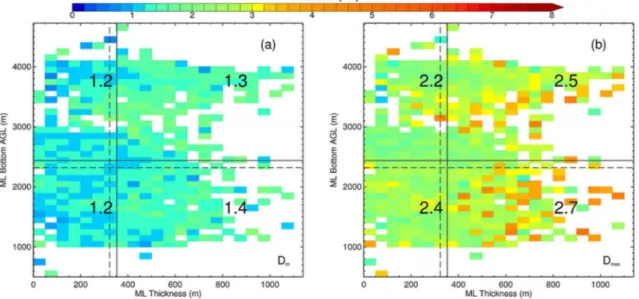
We also examine the combined effects of a lowering and thickening ML on raindrop size measured at the ground. Figure 3 confirms that the lowest and, especially, thickest MLs are associated with the largest raindrops in stratiform precipitation. The Dm measurements are partitioned into
quadrants based on mean ML characteristics and student’s t-tests of the drop size characteristics in each quadrant are conducted to determine whether the RSDs in each quadrant were sampled from the same drop population. The results suggest a statistically significant (probability >0.95) difference between the drop size characteristics (i.e., Dm and Dmax) of the RSDs observed while the ML is thicker
than 315 m compared to those observed when the ML is thinner than 315 m. However, disdrometer observations collected when the ML bottom was lower or higher than the median height of 2310 m AGL is very similar between the two sets of Dm samples. In contrast, the Dmax sample observed during
Figure 2. Polarimetric radar-based melting layer (ML) characteristics and two-dimensional video disdrometers (2DVD) measuredDm from the Huntsville, Alabama and IFloodS stratiform rainfall cases. Relative frequency distribution of (a) ML thickness and (b) ML bottom, respectively, and the solid curve represents the cumulative frequency distribution; (c,d) are box and whiskers plots ofDm corresponding to the ML thickness and ML bottom, respectively, where each box is bounded by the 25th and 75th quartiles and the mean value in eachDmbin is represented by an “X.” The whiskers indicate extremes and extend to 1.5 times the interquartile range. Outliers (i.e., values exceeding 1.5 times the interquartile range) are represented by circles. The dashed line in (c) represents the best fit line from linear least squares regression whereDmis the dependent variable and the ML thickness (∆H in km) is the independent variable.
We also examine the combined effects of a lowering and thickening ML on raindrop size measured at the ground. Figure3confirms that the lowest and, especially, thickest MLs are associated with the largest raindrops in stratiform precipitation. TheDmmeasurements are partitioned into quadrants based on mean ML characteristics and student’st-tests of the drop size characteristics in each quadrant are conducted to determine whether the RSDs in each quadrant were sampled from the same drop population. The results suggest a statistically significant (probability >0.95) difference between the drop size characteristics (i.e.,Dmand Dmax) of the RSDs observed while the ML is thicker than 315 m
compared to those observed when the ML is thinner than 315 m. However, disdrometer observations collected when the ML bottom was lower or higher than the median height of 2310 m AGL is very similar between the two sets ofDmsamples. In contrast, the Dmaxsample observed during low MLs
(i.e., <2310 m AGL) are larger than the Dmaxsampled during high MLs. We attribute this to the
different types of stratiform precipitation events observed (i.e., MCCs versus tropical cyclone versus mid-latitude cyclone). Furthermore, Dmaxexhibits a larger relative increase thanDmas the ML lowers and thickens.
Atmosphere 2018, 9, x FOR PEER REVIEW 8 of 17
low MLs (i.e., <2310 m AGL) are larger than the Dmax sampled during high MLs. We attribute this to
the different types of stratiform precipitation events observed (i.e., MCCs versus tropical cyclone versus mid-latitude cyclone). Furthermore, Dmax exhibits a larger relative increase than Dm as the ML
lowers and thickens.
Figure 3. The (a) mean Dm and (b) maximum Dmax at the ground from 2DVD measurements of rainfall
as a function of the overlying melting layer thickness and its height above ground (i.e., ML bottom). The mean values of Dm and Dmax (mm) inside each quadrant of the ML thickness and ML bottom space
are given. The mean (median) of the ML measurements are indicated by the solid (dashed) lines. 3.2. Evolution of the Raindrop Size Distribution in the Vertical Column
Vertical profiles of Dm below the ML bottom are retrieved above the aforementioned 2DVDs at
15 km range from 2492 min of ARMOR RHI scans and 402 min of NPOL RHI scans during 40 stratiform rainfall events. Increasing Dm trends in the profiles are observed to occur with a lowering
and thickening of the ML, similar to that observed in the ground-based measurements (c.f., Figure 2). A 27% increase in the profile-averaged Dm occurs as the ML thickens from 50 m to 750 m (Table 3).
Table 3. Overview of Dm retrievals from radar RHI scans during periods of varying ML thickness. The angle brackets represent the arithmetic mean of the retrieved profile and σ is its standard deviation.
ML Thickness (m) Number of RHI Profiles <Dm> ± σ(Dm) (mm)
50 ≤ MLthick < 150 m 384 1.40 ± 0.34 150 ≤ MLthick < 250 m 665 1.47 ± 0.31 250 ≤ MLthick < 350 m 697 1.49 ± 0.30 350 ≤ MLthick < 450 m 601 1.57 ± 0.32 450 ≤ MLthick < 550 m 423 1.62 ± 0.32 550 ≤ MLthick < 650 m 295 1.71 ± 0.30 650 ≤ MLthick < 750 m 172 1.78 ± 0.28
Figure 4 shows the column vertical evolution of Dm for the range of ML thicknesses given in
Table 3. A minimum of 100 Dm retrievals were required in each 250 m layer to construct the profiles
in Figure 4 and all points in the profile are at least 250 m below the polarimetric radar-identified ML bottom. Although there is relatively little variation in the mean Dm from the ML bottom to the ground,
especially below 1250 m AGL, the entire Dm profile shifts from 1.3 to 1.4 mm for 50–250 m thick MLs
to 1.7–1.8 mm for 650–750 m thick MLs (Figure 4a). Most of the vertical change in the Dm occurred
within the first 1000–1500 m below the ML. A slight decrease of Dm occurred near the very top of the
profiles.
Figure 3.The (a) meanDmand (b) maximum Dmaxat the ground from 2DVD measurements of rainfall as a function of the overlying melting layer thickness and its height above ground (i.e., ML bottom). The mean values ofDmand Dmax(mm) inside each quadrant of the ML thickness and ML bottom space are given. The mean (median) of the ML measurements are indicated by the solid (dashed) lines. 3.2. Evolution of the Raindrop Size Distribution in the Vertical Column
Vertical profiles ofDmbelow the ML bottom are retrieved above the aforementioned 2DVDs at 15 km range from 2492 min of ARMOR RHI scans and 402 min of NPOL RHI scans during 40 stratiform rainfall events. IncreasingDmtrends in the profiles are observed to occur with a lowering and thickening of the ML, similar to that observed in the ground-based measurements (c.f., Figure2). A 27% increase in the profile-averagedDmoccurs as the ML thickens from 50 m to 750 m (Table3).
Table 3. Overview ofDmretrievals from radar RHI scans during periods of varying ML thickness. The angle brackets represent the arithmetic mean of the retrieved profile andσis its standard deviation.
ML Thickness (m) Number of RHI Profiles <Dm>±σ(Dm) (mm)
50≤MLthick< 150 m 384 1.40±0.34 150≤MLthick< 250 m 665 1.47±0.31 250≤MLthick< 350 m 697 1.49±0.30 350≤MLthick< 450 m 601 1.57±0.32 450≤MLthick< 550 m 423 1.62±0.32 550≤MLthick< 650 m 295 1.71±0.30 650≤MLthick< 750 m 172 1.78±0.28
Figure4shows the column vertical evolution ofDmfor the range of ML thicknesses given in Table3. A minimum of 100Dmretrievals were required in each 250 m layer to construct the profiles in Figure4and all points in the profile are at least 250 m below the polarimetric radar-identified ML bottom. Although there is relatively little variation in the meanDmfrom the ML bottom to the ground, especially below 1250 m AGL, the entireDmprofile shifts from 1.3 to 1.4 mm for 50–250 m thick MLs to 1.7–1.8 mm for 650–750 m thick MLs (Figure4a). Most of the vertical change in theDmoccurred within the first 1000–1500 m below the ML. A slight decrease ofDmoccurred near the very top of the profiles.
Atmosphere 2018, 9, x FOR PEER REVIEW 9 of 17
Figure 4. Vertical profile of (a) mean Dm and (b) standard deviation of Dm retrieved from dual-polarimetric radar measurements for the ML thicknesses listed in Table 3. The legend in the lower-left corners gives the radar-based ML thickness corresponding to each Dm profile.
The peak in mean Dm aloft is 7–12% greater than that at 250 m AGL and becomes less pronounced
but spans a greater vertical distance (i.e., larger raindrops are present throughout a greater depth of the rain layer) as the ML thickens. However, for Dm around 1.3–2.0 mm, the radar retrieval is only
accurate to within 8%, and thus it is difficult to say with a high degree of certainty that the Dm peak
aloft depicts an actual microphysical process. Since this peak in Dm aloft occurs across the entire range
of ML thicknesses as well as the lower and upper quartiles of Dm, we do not believe that the behavior
can be attributed entirely to error in the retrieval (i.e., some portion of the signal is likely physical in nature). This will be further addressed in the discussion section below.
The thicker MLs tend to exhibit less Dm variability in the column below the ML. The standard
deviation of the Dm profile beneath the 650–750 m thick ML is less than that of the thinnest ML at all
heights and by as much as 30% above 2000 m AGL (Figure 4b). The standard deviation of the Dm
profiles increases toward the ground, perhaps indicative of the Dm being further shaped as a result of
collisions as well as evaporative effects.
The Dm profile just above the surface is slightly larger than that recorded by the 2DVD under
similar ML characteristics. This somewhat decreasing Dm trend in the lowest 250–500 m AGL is
indicated by Figure 4a. This difference could also be that the radar, which has a much larger sampling volume than the 2DVD, is detecting more numerous large drops than the 2DVD. Regardless, the radar-retrieved Dm trends with varying ML thickness are similar to the Dm behavior we find at the
ground with the 2DVDs.
4. Discussion
The results provide very strong evidence that the size of raindrops reaching the ground tends to increase as the ML becomes thicker and closer to the ground. Supporting this conclusion, more than 2200 min of polarimetric radar RHI scans were conducted over 2DVDs and used to investigate the response of the raindrop sizes to changes in the thickness and height of the ML. We conducted this study to explicitly test the hypothesis that a thicker and lower ML produces larger raindrops at the ground, which has implications for radar rainfall estimation [14,16]. Although numerous observational studies suggest such a hypothesis is valid [14,65,67–69], most of the aforementioned studies used a reflectivity-based bright band to infer ML characteristics and very few had access to high quality disdrometer measurements. The dual-polarimetric methods used herein for identifying the ML boundaries yielded results that are consistent with particle images obtained through the ML [63,70–73]. Conversely, the bright band is thicker than the dual-polarimetric ML signatures by nearly 200 m. This reflectivity-associated bias in ML thickness relative to the polarimetric methodology likely reflects the strong dependence of reflectivity on hydrometeor size. Aircraft observations
Figure 4. Vertical profile of (a) mean Dm and (b) standard deviation of Dm retrieved from dual-polarimetric radar measurements for the ML thicknesses listed in Table3. The legend in the lower-left corners gives the radar-based ML thickness corresponding to eachDmprofile.
The peak in meanDmaloft is 7–12% greater than that at 250 m AGL and becomes less pronounced but spans a greater vertical distance (i.e., larger raindrops are present throughout a greater depth of the rain layer) as the ML thickens. However, forDmaround 1.3–2.0 mm, the radar retrieval is only accurate to within 8%, and thus it is difficult to say with a high degree of certainty that theDmpeak aloft depicts an actual microphysical process. Since this peak inDmaloft occurs across the entire range of ML thicknesses as well as the lower and upper quartiles ofDm, we do not believe that the behavior can be attributed entirely to error in the retrieval (i.e., some portion of the signal is likely physical in nature). This will be further addressed in the discussion section below.
The thicker MLs tend to exhibit lessDmvariability in the column below the ML. The standard deviation of theDmprofile beneath the 650–750 m thick ML is less than that of the thinnest ML at all heights and by as much as 30% above 2000 m AGL (Figure4b). The standard deviation of theDm
profiles increases toward the ground, perhaps indicative of theDmbeing further shaped as a result of collisions as well as evaporative effects.
TheDmprofile just above the surface is slightly larger than that recorded by the 2DVD under similar ML characteristics. This somewhat decreasing Dm trend in the lowest 250–500 m AGL is indicated by Figure4a. This difference could also be that the radar, which has a much larger sampling volume than the 2DVD, is detecting more numerous large drops than the 2DVD. Regardless, the radar-retrievedDmtrends with varying ML thickness are similar to theDmbehavior we find at the ground with the 2DVDs.
4. Discussion
The results provide very strong evidence that the size of raindrops reaching the ground tends to increase as the ML becomes thicker and closer to the ground. Supporting this conclusion, more than 2200 min of polarimetric radar RHI scans were conducted over 2DVDs and used to investigate the response of the raindrop sizes to changes in the thickness and height of the ML. We conducted this study to explicitly test the hypothesis that a thicker and lower ML produces larger raindrops at the ground, which has implications for radar rainfall estimation [14,16]. Although numerous observational studies suggest such a hypothesis is valid [14,65,67–69], most of the aforementioned studies used a reflectivity-based bright band to infer ML characteristics and very few had access to high quality disdrometer measurements. The dual-polarimetric methods used herein for identifying the ML boundaries yielded results that are consistent with particle images obtained through the ML [63,70–73]. Conversely, the bright band is thicker than the dual-polarimetric ML signatures by nearly 200 m. This reflectivity-associated bias in ML thickness relative to the polarimetric methodology likely reflects the strong dependence of reflectivity on hydrometeor size. Aircraft observations indicate that the radar bright band signature can include very large aggregates present just above the 0◦C level and very large raindrops just below the ML [63,71,73]. Those observations are also consistent with a reflectivity-based ML estimate (i.e., bright band) being thicker than the ML estimated from the dual-polarimetric measurements.
Our results show that the mass-weighted mean raindrop diameter increases as the ML thickens (i.e., increase of distance it takes for snow particles to fully melt), which can be tied to an increase in the overall size of snowflake aggregates above the ML. This is because the rate of snowflake melting is dependent upon its initial size, with larger aggregates having to traverse a further distance before fully melting [70,71,74]. So a thickening of the ML can indicate enhanced aggregation above or near the top of the ML [63]. This is also suggested by the vertically pointing radar observations shown in Figure1in which enhanced low-level reflectivity during times of thicker bright bands are seemingly connected to a less, but locally enhanced, layer of reflectivity above the ML that occurs in a temperature zone that favors growth of dendrites whose fall speed and geometry are very conducive to aggregation [12]. Furthermore, large aggregates can contain more liquid water than smaller, individual ice crystals and upon melting result in a larger raindrop. Thus larger raindrops are expected to occur beneath thicker regions of the ML, suggesting that raindrop size is tied to the efficiency of snowflake aggregation [42,63].
Numerous studies have shown that processes such as breakup and aggregation within the ML are also responsible for shaping the RSD [63,69,71–73,75]. Although no in-situ observations within the ML were available for the cases examined in this study, the UAH XPR measurements during our stratiform precipitation events are used to infer the dominance of aggregation or breakup within the ML by examining the ratio of the particle flux above and below the ML, where particle flux is estimated by the product of equivalent reflectivity and vertical velocity [75]. Aggregation dominates over breakup within the ML if this ratio is less than 0.23 [75]. Figure5reveals that the ML thickens as the particle flux ratio decreases (i.e., aggregation becomes more dominant) within the ML, which is consistent with the bright band observations by Reference [69]. Thus an increase in the mean raindrop size is not only
Atmosphere2018,9, 319 11 of 18
associated with enhanced aggregation above the ML but also enhanced aggregation within the ML consistent with the in situ observations through the ML by Reference [73].
indicate that the radar bright band signature can include very large aggregates present just above the 0 °C level and very large raindrops just below the ML [63,71,73]. Those observations are also consistent with a reflectivity-based ML estimate (i.e., bright band) being thicker than the ML estimated from the dual-polarimetric measurements.
Our results show that the mass-weighted mean raindrop diameter increases as the ML thickens (i.e., increase of distance it takes for snow particles to fully melt), which can be tied to an increase in the overall size of snowflake aggregates above the ML. This is because the rate of snowflake melting is dependent upon its initial size, with larger aggregates having to traverse a further distance before fully melting [70,71,74]. So a thickening of the ML can indicate enhanced aggregation above or near the top of the ML [63]. This is also suggested by the vertically pointing radar observations shown in Figure 1 in which enhanced low-level reflectivity during times of thicker bright bands are seemingly connected to a less, but locally enhanced, layer of reflectivity above the ML that occurs in a temperature zone that favors growth of dendrites whose fall speed and geometry are very conducive to aggregation [12]. Furthermore, large aggregates can contain more liquid water than smaller, individual ice crystals and upon melting result in a larger raindrop. Thus larger raindrops are expected to occur beneath thicker regions of the ML, suggesting that raindrop size is tied to the efficiency of snowflake aggregation [42,63].
Numerous studies have shown that processes such as breakup and aggregation within the ML are also responsible for shaping the RSD [63,69,71–73,75]. Although no in-situ observations within the ML were available for the cases examined in this study, the UAH XPR measurements during our stratiform precipitation events are used to infer the dominance of aggregation or breakup within the ML by examining the ratio of the particle flux above and below the ML, where particle flux is estimated by the product of equivalent reflectivity and vertical velocity [75]. Aggregation dominates over breakup within the ML if this ratio is less than 0.23 [75]. Figure 5 reveals that the ML thickens as the particle flux ratio decreases (i.e., aggregation becomes more dominant) within the ML, which is consistent with the bright band observations by Reference [69]. Thus an increase in the mean raindrop size is not only associated with enhanced aggregation above the ML but also enhanced aggregation within the ML consistent with the in situ observations through the ML by Reference [73].
Figure 5. Box and whisker type plot with statistics represented similar to Figure 2 but showing particle flux across the ML as a function of ML thickness estimated from the XPR measurements in Huntsville, Alabama. The dashed line delineates MLs dominated by aggregation or breakup. The relative frequency of profiles in each ML thickness bin is indicated by the percentages.
Figure 5.Box and whisker type plot with statistics represented similar to Figure2but showing particle flux across the ML as a function of ML thickness estimated from the XPR measurements in Huntsville, Alabama. The dashed line delineates MLs dominated by aggregation or breakup. The relative frequency of profiles in each ML thickness bin is indicated by the percentages.
We find that the largest raindrops exist primarily beneath thick MLs and/or those MLs occurring closest to the ground. For the MLs close to the ground, the shorter fall distance reduces (1) the chance for breakup and (2) the total amount of liquid water that is evaporated. The increase of mean raindrop size as the ML lowers is consistent with the observations made by Reference [69] during descending bright band periods of a landfalling tropical storm rain band.
Relatively little variation of theDmwith height is found in stratiform precipitation events, which is consistent with previous findings [76,77]. Within a given stratiform event, a thickening and lowering of the ML shifts and compresses the vertical profile ofDmbut does not significantly alter its basic shape. The mean raindrop size at the ground is similar to that just below the ML andDmchanges no more than 12% (i.e., <0.2 mm) throughout the vertical profile. The largest values ofDmare found about 1000 m below each ML regardless of its thickness (i.e., it cannot be accounted for by changes within the ML). This is also around the height where a maximum D0was observed in a widespread stratiform
rain case over southeast India [77] and in a stratiform event over eastern China [78]. The enhanced Dmaloft is believed to be due to a physical process that occurs in stratiform rainfall and not just radar retrieval error. TheDmpeak may be an indicator of a region of drier air aloft (e.g., the “onion” shaped soundings measured by Reference [79] and hence evaporation in the trailing stratiform region of squall lines), which has implications for dual-polarimetric radar rainfall estimation [80]. The datasets gathered for this study do not provide the necessary information to assess if this is indeed the case. The enhancedDmaloft may be an additional source of error in radar rainfall estimates, similar to the bright band but likely not as significant, except perhaps for very light rainfall rates where the bright band is not as strong.
The trends in Dmaxcompared to those we found forDmsuggest that the tail of the RSD is much more affected by changes in the ML characteristics. Consequently, radar rainfall estimators based on reflectivity (i.e., highly sensitive to the tail of the RSD) should be correspondingly more variable
with changes in ML thickness and height compared to those estimators that utilize specific differential phase (KDP) and differential reflectivity (ZDR) that are less sensitive to Dmax.
5. Summary and Conclusions
The motivation for this study is to improve radar-based QPE by considering the vertical variability of precipitation that complicates accurate retrieval of rainfall near the surface, especially at relatively far distances from the radar. We considered how precipitation ML characteristics impact the physics of rainfall development in the vertical column. Our focus on the melting layer is due to the fact that it is usually a rather prominent feature of stratiform precipitation and can be readily mapped with radar (ground-, aircraft-, or space-based). To do this we examined the evolution of the RSD under different melting layers and found that variations inDmof stratiform precipitation tended to follow variations in the ML thickness. A hypothesis is that thicker and lower MLs are associated with larger raindrops at the ground. Instead of relying solely on the radar reflectivity bright band, which is a radar manifestation of the melting layer and is thicker than the true melting layer, to quantify this relationship as was done in past studies [14,69], we used high-resolution polarimetric radar scans to identify ML boundaries, focusing in particular onρhvmeasurements, which provide a rather accurate depiction of melting hydrometeors [29,33,38,39].
We found a direct linear relationship (correlation of 0.94) between the thickness of the ML and the size of raindrops measured at the ground with 2DVDs. Variations in ML thickness were found to describe nearly 90% of the variability in raindrop size. For two tropical rainfall events, we found a strong inverse relationship exists between the raindrop size and height of the ML. Such similarity is not very surprising since the ML thickness is governed by the distance it takes a snowflake to melt. This in turn can cause the bottom of the ML to descend while its top remains around the same altitude (i.e., ML thickens).
One caveat that might impact this strong ML-RSD relationship we find is that ourDmmay be an overestimate since the 2DVD has been reported to underestimate the number of small (equivalent spherical diameter < 0.7 mm) drops [81]. However, this reportedDmbias is most pronounced only in light rainfall events when a relatively thick bright band is not present [81]. Hence, we anticipate a good correlation to exist betweenDmand ML thickness for stratiform precipitation but are somewhat uncertain about the strength of that relationship for very light stratiform rainfall (R < 0.5 mm/h) when smaller drops are often present.
We also examined the variability ofDmup the column with respect to changes in the ML. We found that on average larger raindrops through the depth of the column occur with thicker MLs. Moreover, the shape of theDmprofile was fairly uniform, exhibiting only minor variations in the vertical such that Dmnear the ground was similar to that below the melting layer. It is still unclear whether increased aggregation aloft and/or within the ML ultimately leads to the thicker ML and larger raindrops- more study on coordinated airborne and multi-parameter radar observations are required. Additionally, the ML effects on other RSD parameters, such asNw, are also needed to assist with interpretation of the microphysical effects that shape the RSD. However, there is typically less confidence in the radar-retrieved value ofNwcompared withDm. High resolution, vertically pointing Doppler radars, such as the Micro Rain Radar [82], would be a good tool to use for further investigating the ML effects on the RSD since they are capable of retrieving both the profiles ofDmandNwas well as the ML characteristics.
The connection between rainfall at the ground and the overlying microphysics in the column provide a means for improving radar QPE at far distances from a given radar.These results have shown definitive proof that a thickening, and to a lesser extent a lowering, of the ML causes an increase in raindrop diameter below the ML that extends to the surface. Thus, information about the thickness and height of the ML may be useful to constrain RSD retrievals and thereby ultimately improve radar rainfall estimation to the extent a rainfall estimation algorithm accounts for potential profile changes in the RSD. For example, space-based radar algorithms developed for use with the Global Precipitation
Measurement (GPM) Mission [83,84] could use theDmprofile trends we find for stratiform precipitation as an additional guide and means to verify, and adjust if necessary, retrieved RSD characteristics in the vertical column.
Author Contributions:Conceptualization, P.N.G. and W.A.P.; Methodology, Investigation and Formal Analysis, P.N.G.; Data Curation, P.N.G, W.A.P., L.D.C. and K.R.K; Writing—Original Draft Preparation, P.N.G.; Writing—Review & Editing, W.A.P., L.D.C. and K.R.K; Visualization, P.N.G.; Supervision, W.A.P.; Resources, W.A.P., L.D.C. and K.R.K.
Funding:This research was funded by the National Aeronautics and Space Administration (NASA) Precipitation Measurement Mission (PMM) and Ground Validation (GV) Programs.
Acknowledgments: P.N.G. was supported by the NASA Pathways Internship Program at NASA’s George C. Marshall Space Flight Center while conducting this study. L.D.C. would like to acknowledge support from NASA PMM and GPM GV via the UAH-NASA Marshall Space Flight Center Cooperative Agreement #NNM1AA01A. We would like to acknowledge V.N. Bringi and M. Thurai for providing the CSU 2DVD data and radar scattering simulation software CANTMAT Version 1.2 that was developed at CSU by C. Tang and V.N. Bringi. We would also like to thank the three anonymous reviewers whose suggestions helped strengthen the manuscript.
Conflicts of Interest:The authors declare no conflict of interest. The funders had no role in the design of this study; in the collection, analyses, or interpretation of its data; in the writing of this manuscript and in the decision to publish these results.
Appendix A
The CANTMAT Version 1.2 software program, which is a Meuller-matrix based approach [1] adopted for calculating radar parameters using the T-matrix method formulation by Reference [52] and was developed at CSU by C. Tang and V.N. Bring, is used for our radar scattering simulations. This scattering simulation tool has been used in numerous polarimetric radar studies, for example, References [48,49,51]. We use the following assumptions in the radar scattering simulations: (1) raindrop shapes from the 80 m bridge experiment [85]; (2) raindrops have a Gaussian canting angle distribution with a mean and standard deviation of 0◦and 8◦, respectively [86]; (3) The maximum diameter,Dmax= 3Dmto be representative of most DSDs, especially those containing large raindrops in light rainfall [44,55,87]; (4) raindrop temperature is represented by the mean hourly temperature near (within 10 m for Huntsville and roughly 10–30 km for Iowa) the location of each 2DVD; and (5) a radar antenna elevation angle of 0◦. Only 1-min spectra containing at least 150 raindrops are used for the scattering simulations to reduce variability in the simulated radar parameters. We add Gaussian noise to the simulated radar parameters for each radar configuration (Table1) following the methods outlined in chapter 6 of [1].
The simulated radar parameters are compared with the 1-min RSD spectra from the 2DVD raindrop measurements to create empirical fits that facilitate retrieving Dm from the radar measurements. In determining the equation for the radar retrieval of the RSD, we randomly select 70% (94,409 min) of the RSD spectra listed in TableA1to computeDmfits for each radar and location. The remaining 30% (40,460 min) are for assessing the uncertainty of the parameterization. We find the following equations provide a good fit for using the differential reflectivity,ZDR, to parameterizeDm: • Alabama (ARMOR):
Dm= 0.5969 + 1.7953ZDR−1.1111ZDR2+ 0.5171ZDR3−0.1360ZDR4+ 0.0142ZDR5,−0.2≤ZDR≤4.7 dB (A1)
• Iowa (NPOL):
Table A1.Overview of 2DVD rainfall measurements collected at Huntsville and IFloodS. This summary includes measurements from multiple 2DVDs when present at the same location.
Location Observation Period (YYYY-MM-DD) Number of Raindrops(n) (in Millions) Total 1-min RSD Spectra (n≥100) Rainfall Rates (mm/h) Total Rainfall (mm) Huntsville, AL (number. of 2DVDs: 4) 2007-07-07 to 2013-12-09 75.3 109,969 0.006–157.4 5903 Eastern Iowa (IFloodS)
(number of 2DVDs: 6)
2013-04-09 to
2013-06-16 16.3 24,900 0.006–121.2 970.5
References
1. Bringi, V.N.; Chandrasekar, V.Polarimetric Doppler Weather Radar: Principles and Applications; Cambridge University Press: Cambridge, UK, 2001; ISBN 0-521-62384-7.
2. Ryzhkov, A.V.; Schuur, T.J.; Burgess, D.W.; Heinselman, P.L.; Giangrande, S.E.; Zrnic, D.S. The Joint Polarization Experiment: Polarimetric rainfall measurements and hydrometeor classification. Bull. Am. Meteorol. Soc.2005,86, 809–824. [CrossRef]
3. Boodoo, S.; Hudak, D.; Ryzhkov, A.; Zhang, P.; Donaldson, N.; Sills, D.; Reid, J.; Boodoo, S.; Hudak, D.; Ryzhkov, A.; et al. Quantitative precipitation estimation from a C-band dual-polarized radar for the 8 July 2013 flood in Toronto, Canada.J. Hydrometeorol.2015,16, 2027–2044. [CrossRef]
4. Ryzhkov, A.V. The Impact of beam broadening on the quality of radar polarimetric data.J. Atmos. Ocean. Technol.2007,24, 729–744. [CrossRef]
5. Villarini, G.; Krajewski, W.F. Review of the different sources of uncertainty in single polarization radar-based estimates of rainfall.Surv. Geophys.2010,31, 107–129. [CrossRef]
6. Gorgucci, E.; Baldini, L. Influence of beam broadening on the accuracy of radar polarimetric rainfall estimation.J. Hydrometeorol.2015,16, 1356–1371. [CrossRef]
7. Joss, J.; Lee, R. The application of radar-gauge comparisons to operational precipitation profile corrections.
J. Appl. Meteorol.1995,34, 2612–2630. [CrossRef]
8. Bellon, A.; Lee, G.W.; Zawadzki, I. Error statistics of VPR corrections in stratiform precipitation. J. Appl. Meteorol.2005,44, 998–1015. [CrossRef]
9. Maahn, M.; Burgard, C.; Crewell, S.; Gorodetskaya, I.V.; Kneifel, S.; Lhermitte, S.; Van Tricht, K.; van Lipzig, N.P.M. How does the spaceborne radar blind zone affect derived surface snowfall statistics in polar regions?J. Geophys. Res. Atmos.2014,119, 13604–13620. [CrossRef]
10. Chandrasekar, V.; Meneghini, R.; Zawadzki, I. Global and local precipitation measurements by radar.
Meteorol. Monogr.2003,30, 215. [CrossRef]
11. Iguchi, T.; Kozu, T.; Kwiatkowski, J.; Meneghini, R.; Awaka, J.; Okamoto, K. Uncertainties in the rain profiling algorithm for the TRMM precipitation radar.J. Meteorol. Soc. Jpn.2009,87A, 1–30. [CrossRef]
12. Pruppacher, H.R.; Klett, J.D.Microphysics of Clouds and Precipitation; Mysak, L.A., Hamilton, K., Eds.; Atmospheric and Oceanographic Sciences Library; Springer: Dordrecht, The Netherlands, 2010; Volume 18, ISBN 978-0-7923-4211-3.
13. Waldvogel, A. TheN0Jump of Raindrop Spectra.J. Atmos. Sci.1974,31, 1067–1078. [CrossRef]
14. Huggel, A.; Schmid, W.; Waldvogel, A. Raindrop size distributions and the radar bright band. J. Appl. Meteorol.1996,35, 1688–1701. [CrossRef]
15. Brandes, E.A.; Zhang, G.; Vivekanandan, J. Drop size distribution retrieval with polarimetric radar: Model and application.J. Appl. Meteorol.2004,43, 461–475. [CrossRef]
16. Sharma, S.; Konwar, M.; Sarma, D.K.; Kalapureddy, M.C.R.; Jain, A.R. Characteristics of rain integral parameters during tropical convective, transition, and stratiform rain at Gadanki and its application in rain retrieval.J. Appl. Meteorol. Climatol.2009,48, 1245–1266. [CrossRef]
17. Andri´c, J.; Kumjian, M.R.; Zrni´c, D.S.; Straka, J.M.; Melnikov, V.M. Polarimetric signatures above the melting layer in winter storms: An observational and modeling study.J. Appl. Meteorol. Climatol.2013,52, 682–700. [CrossRef]
18. Yoshikawa, E.; Kida, S.; Yoshida, S.; Morimoto, T.; Ushio, T.; Kawasaki, Z. Vertical structure of raindrop size distribution in lower atmospheric boundary layer.Geophys. Res. Lett.2010,37. [CrossRef]
19. Oue, M.; Uyeda, H.; Shusse, Y. Two types of precipitation particle distribution in convective cells accompanying a Baiu frontal rainband around Okinawa Island, Japan.J. Geophys. Res.2010,115, D02201. [CrossRef]
20. Kim, D.-K.; Kim, Y.-H.; Chang, D.-E. A study of microphysical properties within a precipitation system using wind profiler spectra.Asia Pac. J. Atmos. Sci.2011,47, 413–420. [CrossRef]
21. Petersen, W.A.; Knupp, K.R. Coauthors The UAH-NSSTC/WHNT ARMOR C-band dual-polarimetric radar: A unique collaboration in research, education and technology transfer. In Proceedings of the 32nd Conference on Radar Meteorology, Albuquerque, NM, USA, 24–29 October 2005; American Meteor Society: Albuquerque, NM, USA, 2005; p. 12R.4.
22. Gerlach, J.; Petersen, W.A. The NASA transportable S-band dual-polarimetric radar. Antenna system upgrades, performance and deployment during MC3E. In Proceedings of the 35th Conference on Radar Meteorology, Pittsburgh, PA, USA, 26–30 September 2011; American Meteorological Society: Pittsburgh, PA, USA, 2011; p. P192.
23. Petersen, W.A.; Krajewski, W. Status update on the GPM Ground Validation Iowa Flood Studies (IFloodS) Field Experiement. InEuropean Geosciences Union General Assembly; European Geosciences Union: Vienna, Austria, 2013.
24. Doviak, R.J.; Bringi, V.; Ryzhkov, A.; Zahrai, A.; Zrni´c, D. Considerations for polarimetric upgrades to operational WSR-88D radars.J. Atmos. Ocean. Technol.2000,17, 257–278. [CrossRef]
25. Scott, R.D.; Krehbiel, P.R.; Rison, W. The use of simultaneous horizontal and vertical transmissions for dual-polarization radar meteorological observations.J. Atmos. Ocean. Technol.2001,18, 629–648. [CrossRef] 26. Kruger, A.; Krajewski, W.F. Two-dimensional video disdrometer: A description.J. Atmos. Ocean. Technol.
2002,19, 602–617. [CrossRef]
27. Schönhuber, M.; Lammer, G.; Randeu, W.L. The 2D-Video-Distrometer. InPrecipitation: Advances in Measurement, Estimation and Prediction; Michaelides, S., Ed.; Springer: Berlin/Heidelberg, Germany, 2008; pp. 3–31. ISBN 978-3-540-77654-3.
28. Matrosov, S.Y.; Clark, K.A.; Kingsmill, D.E. A polarimetric radar approach to identify rain, melting-layer, and snow regions for applying corrections to vertical profiles of reflectivity.J. Appl. Meteorol. Climatol.2007,
46, 154–166. [CrossRef]
29. Giangrande, S.E.; Krause, J.M.; Ryzhkov, A.V. Automatic designation of the melting layer with a polarimetric prototype of the WSR-88D radar.J. Appl. Meteorol. Climatol.2008,47, 1354–1364. [CrossRef]
30. Shusse, Y.; Nakagawa, K.; Takahashi, N.; Satoh, S.; Iguchi, T. Characteristics of polarimetric radar variables in three types of rainfalls in a Baiu front event over the East China Sea.J. Meteorol. Soc. Jpn.2009,87, 865–875. [CrossRef]
31. Boodoo, S.; Hudak, D.; Donaldson, N.; Leduc, M. Application of dual-polarization radar melting-layer detection algorithm.J. Appl. Meteorol. Climatol.2010,49, 1779–1793. [CrossRef]
32. Wolfensberger, D.; Scipion, D.; Berne, A. Detection and characterization of the melting layer based on polarimetric radar scans.Q. J. R. Meteorol. Soc.2016,142, 108–124. [CrossRef]
33. Caylor, I.J.; Illingworth, A.J. Identification of the bright band and hydrometeors using co-polar dual polarization radar. In Proceedings of the Preprints, 24th American Meteorological Socienty Conference on Radar Meteorology, Tallahassee, FL, USA, 27–31 March 1989; American Meteorological Society: Boston, MA, USA, 1989; pp. 9–12.
34. Balakrishnan, N.; Zrnic, D.S. Use of polarization to characterize precipitation and discriminate large hail.
J. Atmos. Sci.1990,47, 1525–1540. [CrossRef]
35. Benjamin, S.G.; Dévényi, D.; Weygandt, S.S.; Brundage, K.J.; Brown, J.M.; Grell, G.A.; Kim, D.; Schwartz, B.E.; Smirnova, T.G.; Smith, T.L.; et al. An Hourly Assimilation–Forecast Cycle: The RUC.Mon. Weather Rev.2004,
132, 495–518. [CrossRef]
36. Aydin, K.; Giridhar, V. C-band dual-polarization radar observables in rain.J. Atmos. Ocean. Technol.1992,
9, 383–390. [CrossRef]
37. Baldini, L.; Gorgucci, E.; Petersen, W. Implementations of CSU hydrometeor classification scheme for C-band polarimetric radars. In Proceedings of the 32nd Conference on Radar Meteorology, Albuquerque, NM, USA, 24–29 October 2005; American Meteor Society: Albuquerque, NM, USA, 2005; p. P11.4.
38. Zrni´c, D.S.; Raghavan, R.; Chandrasekar, V. Observations of copolar correlation coefficient through a bright band at vertical incidence.J. Appl. Meteorol.1994,33, 45–52. [CrossRef]
39. Brandes, E.A.; Ikeda, K. Freezing-level estimation with polarimetric radar.J. Appl. Meteorol.2004,43, 1541–1553. [CrossRef]
40. Marshall, J.S. Precipitation trajectories and patterns.J. Meteorol.1953,10, 25–29. [CrossRef]
41. Gunn, R.E.S.; Marshall, J.S. The effect of wind shear on falling precipitation.J. Meteorol.1955,12, 339–349. [CrossRef]
42. Yuter, S.E.; Houze, R.A. Measurements of raindrop size distributions over the Pacific warm pool and implications for Z-R relations.J. Appl. Meteorol.1997,36, 847–867. [CrossRef]
43. Kumjian, M.R.; Ryzhkov, A.V. The impact of size sorting on the polarimetric radar variables.J. Atmos. Sci.
2012,69, 2042–2060. [CrossRef]
44. Gatlin, P.N.; Thurai, M.; Bringi, V.N.; Petersen, W.A.; Wolff, D.B.; Tokay, A.; Carey, L.D.; Wingo, M.; Thurai, M.; Petersen, W.A.; et al. Searching for large raindrops: A global summary of two-dimensional video disdrometer observations.J. Appl. Meteorol. Climatol.2014, 1069–1089. [CrossRef]
45. Testud, J.; Oury, S.; Black, R.A.; Amayenc, P.; Dou, X.; Testud, J.; Oury, S.; Black, R.A.; Amayenc, P.; Dou, X. The concept of “normalized” distribution to describe raindrop spectra: A tool for cloud physics and cloud remote sensing.J. Appl. Meteorol.2001,40, 1118–1140. [CrossRef]
46. Bringi, V.N.; Chandrasekar, V.; Hubbert, J.; Gorgucci, E.; Randeu, W.L.; Schoenhuber, M.; Bringi, V.N.; Chandrasekar, V.; Hubbert, J.; Gorgucci, E.; et al. Raindrop size distribution in different climatic regimes from disdrometer and dual-polarized radar analysis.J. Atmos. Sci.2003,60, 354–365. [CrossRef]
47. Bringi, V.N.; Keenan, T.D.; Chandrasekar, V. Correcting C-band radar reflectivity and differential reflectivity data for rain attenuation: A self-consistent method with constraints.IEEE Trans. Geosci. Remote Sens.2001,
39, 1906–1915. [CrossRef]
48. Bringi, V.N.; Rasmussen, R.M.; Vivekanandan, J. Multiparameter Radar Measurements in Colorado Convective Storms. Part I: Graupel Melting Studies.J. Atmos. Sci.1986,43, 2545–2563. [CrossRef]
49. Vivekanandan, J.; Adams, W.M.; Bringi, V.N. Rigorous Approach to Polarimetric Radar Modeling of Hydrometeor Orientation Distributions.J. Appl. Meteorol.1991,30, 1053–1063. [CrossRef]
50. Zhang, G.; Vivekanandan, J.; Brandes, E. A method for estimating rain rate and drop size distribution from polarimetric radar measurements.IEEE Trans. Geosci. Remote Sens.2001,39, 830–841. [CrossRef]
51. Thurai, M.; Huang, G.J.; Bringi, V.N.; Randeu, W.L.; Schönhuber, M.; Thurai, M.; Huang, G.J.; Bringi, V.N.; Randeu, W.L.; Schönhuber, M. Drop shapes, model comparisons, and calculations of polarimetric radar parameters in rain.J. Atmos. Ocean. Technol.2007,24, 1019–1032. [CrossRef]
52. Barber, P.; Yeh, C. Scattering of electromagnetic waves by arbitrarily shaped dielectric bodies.Appl. Opt.
1975,14, 2864. [CrossRef] [PubMed]
53. Mishchenko, M.I.; Travis, L.D. Capabilities and limitations of a current FORTRAN implementation of the T-matrix method for randomly oriented, rotationally symmetric scatterers.J. Quant. Spectrosc. Radiat. Transf.
1998,60, 309–324. [CrossRef]
54. Petersen, W.; Carey, L.D.; Gatlin, P.N.; Wingo, M.T.; Wolff, D.B.; Bringi, V.N. Drop size distribution measurements supporting the NASA Global Precipitation Measurement Mission: Infrastructure and preliminary results. In Proceedings of the 35th Conference on Radar Meteorology, Pittsburgh, PA, USA, 26–30 September 2011; American Meteorological Society: Pittsburgh, PA, USA, 2011; p. P36.
55. Carey, L.D.; Petersen, W.A. Sensitivity of C-band polarimetric radar–based drop size estimates to maximum diameter.J. Appl. Meteorol. Climatol.2015,54, 1352–1371. [CrossRef]
56. Gorgucci, E.; Chandrasekar, V.; Bringi, V.N.; Scarchilli, G. Estimation of raindrop size distribution parameters from polarimetric radar measurements.J. Atmos. Sci.2002,59, 2373–2384. [CrossRef]
57. Brandes, E.A.; Zhang, G.; Vivekanandan, J. An evaluation of a drop distribution–based polarimetric radar rainfall estimator.J. Appl. Meteorol.2003,42, 652–660. [CrossRef]
58. Thurai, M.; Bringi, V.N.; Carey, L.D.; Gatlin, P.; Schultz, E.; Petersen, W.A. Estimating the accuracy of polarimetric radar–based retrievals of drop-size distribution parameters and rain rate: An application of error variance separation using radar-derived spatial correlations. J. Hydrometeorol. 2012,13, 1066–1079. [CrossRef]
59. Bringi, V.N.; Thurai, M.; Nakagawa, K.; Huang, G.J.; Kobayahsi, T.; Adachi, A.; Hanando, H.; Seizawa, S. Rainfall Estimation from C-Band Polarimetric Radar in Okinawa, Japan: Comparisons with 2D-Video Disdrometer and 400 MHz Wind Profiler.J. Meteorol. Soc. Jpn.2006,84, 705–724. [CrossRef]