PDF hosted at the Radboud Repository of the Radboud University
Nijmegen
The following full text is a preprint version which may differ from the publisher's version.
For additional information about this publication click this link.
http://hdl.handle.net/2066/197099
Please be advised that this information was generated on 2019-06-02 and may be subject to
change.
How to Train Your Speaker Embeddings Extractor
Mitchell McLaren
1, Diego Castan
1, Mahesh Kumar Nandwana
1, Luciana Ferrer
2, Emre Yılmaz
31
Speech Technology and Research Laboratory, SRI International, California, USA
2Instituto de Investigaci´on en Ciencias de la Computaci´on, UBA-CONICET, Argentina
3
CLS/CLST, Radboud University, Nijmegen, The Netherlands
{mitchell.mclaren, diego.castan, mahesh.nandwana}@sri.com
,
[email protected], [email protected]Abstract
With the recent introduction of speaker embeddings for text-independent speaker recognition, many fundamen-tal questions require addressing in order to fast-track the development of this new era of technology. Of particu-lar interest is the ability of the speaker embeddings net-work to leverage artificially degraded data at a far greater rate beyond prior technologies, even in the evaluation of naturally degraded data. In this study, we aim to ex-plore some of the fundamental requirements for build-ing a good speaker embeddbuild-ings extractor. We analyze the impact of voice activity detection, types of degrada-tion, the amount of degraded data, and number of speak-ers required for a good network. These aspects are ana-lyzed over a large set of 11 conditions from 7 evaluation datasets. We lay out a set of recommendations for train-ing the network based on the observed trends. By apply-ing these recommendations to enhance the default recipe provided in the Kaldi toolkit, a significant gain of 13-21% on the Speakers in the Wild and NIST SRE’16 datasets is achieved.
1. Introduction
In recent years, the use of deep neural networks (DNNs) in speaker recognition has progressed rapidly with the in-troduction of automatic speech recognition (ASR) DNNs to replace the role of the universal background model (UBM) [1], the use of bottleneck features in combina-tion with tradicombina-tional features [2], the use of d-vectors for text-dependent speaker identification (SID) [3], and more recently, the use of x-vectors or speaker embeddings for text-independent SID [4, 5, 6]. This article focuses on the speaker embeddings technology, which has proven to provide a significant gain over prior technology (DNN-based i-vectors) along with the ability to generalize more readily to unseen audio conditions.
Along with the new technology comes many open av-enues for driving the research forward. Prior to exploring these research avenues, numerous fundamental questions require exploration to provide a reasonable grounding
into what forms a solid baseline or standard system train-ing approach. For the research community, the publicly-available Kaldi software provides a recipe for training a good embeddings extractor [7]. This recipe, however, re-lies on numerous datasets available under LDC license, preventing research groups without licenses from pro-gressing from using the recipe as a starting point. To help understand the data needs of the embeddings DNN, our main focus in this article is on the quality and quantity of data used for this purpose. As prior publications have already demonstrated the strength of embeddings com-pared to i-vectors [5, 6], we restrain the scope of this work to the embeddings framework alone.
In this study, we aim to answer the question of how to train a robust speaker embeddings extractor. Trends are analyzed using the PRISM training set for the DNN and evaluated on 11 conditions from 7 different datasets for a thorough analysis. We start by analyzing the impact of voice activity detection during training and evaluation of the embeddings network. We then investigate the im-pact of varying the degree of degradations in the network training to find a inflection point at which the network starts to degrade. Additionally, we analyze the relative impact of each type of degradation from noise, music, reverb, and audio compression. Once we define a ro-bust degradation protocol, we analyze how many speak-ers and copies of degraded data are required to produce a good embeddings extractor. We also briefly consider the impact of minibatch size during training. The trends and findings observed in the study are concisely laid out as a set of recommendations for training a speaker em-beddings SID system. These recommendations are then used to enhance the default recipe provided in Kaldi and benchmarked on the SRE’16 [8] and Speakers in the Wild (SITW) [9] datasets.
2. System Setup
We start with the default Kaldi recipe [7], keeping the DNN parameters fixed for the entirety of this study, to enable focusing on the extractor’s data needs. This is based on the assumption that the Kaldi team have
al-ready roughly tuned the parameters of the embeddings recipe. The embeddings network starts with five frame-level hidden layers, all using rectified linear unit (ReLU) activation and batch normalization [10]. The first three layers incrementally add time context with stacking of [-2,-1,0,1,2], [-2,0,2], and [-3,0,3] instances of the input frame. A statistics pooling layer then stacks the mean and standard deviation of the frames per audio segment, resulting in a 3000 dimensional segment-level represen-tation. The final two hidden layers of 512 nodes op-erate at the segment-level and use ReLU activation and batch normalization prior to the output layer, which tar-gets speaker labels for each audio segment using log soft-max as the output. The embeddings are extracted from the first segment-level hidden layer of 512 nodes.
In contrast to the default Kaldi recipe, we replace the Mel frequency cepstral coefficients (MFCC) features, speech activity detection (SAD), and audio-degradation process from Kaldi with our own, while leveraging Kaldi for producing DNN training audio chunks of 2–4 sec-onds of speech each, shuffling them, and training the DNN. Once trained, we use our Python tools to train a gender-independent probabilistic linear discriminant analysis (PLDA) model and evaluate numerous datasets for a thorough benchmark of each DNN. Our SAD is based on a DNN with two hidden layers with 500/100 nodes, respectively, and used 20-dimensional MFCC fea-tures, stacked with 31 frames, and mean and variance normalization over a 201-frame window. The optimal threshold found using an i-vector framework over a large development set was found to be 0.5.
2.1. Training Data
We focus on a subset of training data provided in the Kaldi recipe [7]. Specifically, we use only the raw audio (without artificial degradation) from the PRISM training lists [11] for DNN training, and the default PRISM ing lists with additional transcoded data for PLDA train-ing [12]. These lists stay constant throughout this study with the exception of the DNN training lists, in which we investigate the adding of artificially degraded copies of the training data as well as the number of speakers in the training set.
2.2. Degradations
We focus on four main types of degradation: (1) reverb, (2) compression, (3) non-vocal music, and (4) noise, which consists of a range of cafe, babble, road, traffic, mechanical, and natural noises. All noises were sourced from freesound.org and are high quality, natural recordings of live environments. All reverb signals were sourced online from echothief.com and represent the true impulse response from real locations. Compres-sion involved using more than 30 different codec-bitrate
pairs per our prior article on compressed speech [12]. Non-vocal music was sourced form a single CD collec-tion of 100 instrumental songs covering a wide range of genres. Noise or music degradations were added to the audio using the Filtering and Noise-adding Toolkit (FaNT), reverb using Fconv, and compression was per-formed using FFmpeg or the tools provided with the codecs themselves.
2.3. Evaluation Data
For evaluation, we use 11 conditions from 7 different datasets, of which 6 are publically available. These are defined in Table 1. For the analysis of discriminative power, we look at the average EER across these sets. We provide the EER performance for each set in the table in order to give readers an idea of the breakdown in per-formance per dataset. The system used to produce these metrics is the best performing system in Section 5.
3. The Role of Speech Activity Detection in
DNN training
An often-overlooked aspect of speech technology is the impact of SAD. In contrast to the i-vector framework with benefits from a strict SAD threshold in both training and testing, we demonstrate in this section that the embed-dings DNN can potentially benefit from a more relaxed threshold during training.
3.1. SAD during DNN training
We start with a SAD threshold of 0.5 that was tuned on our i-vector pipeline. DNNs are known to require large amounts of training data and, in the case of em-beddings, benefit from artificial degradations [6]. Given this information, one of the easiest ways to provide more data for DNN training is reducing the SAD threshold to provide more speech frames. This obviously has the potential drawback of providing fewer voiced or noise frames to the DNN training. However, given the embed-dings DNN uses a statistics pooling layer that summa-rizes training segments between 200–400 frames, so long as there is sufficient speech within each segment such that the speaker identity can be extracted, then having fewer speech-like frames is a natural way to produce noisier segments in DNN training. The assumption is that these noisier frames will force the DNN to focus on the cru-cial aspects within the hidden layers in order to extract the speaker information in the context of noise and other degradations.
Along with the changing the SAD threshold, we in-vestigated the use of supplying the SAD log-likelihood ratio (LLR) at the input of the DNN along with the MFCC input features in anticipation of the DNN leveraging this information to appropriately weight each frame based on the speech LLR. In this case, we still applied a hard SAD
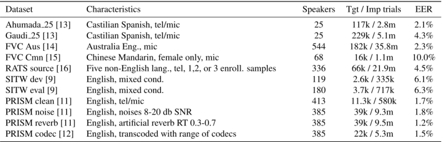
Table 1: The evaluation datasets with corresponding characteristics and target/impostor (tgt/imp) trial counts used in this study. The first five datasets, had audio cut to 10, 20, 30, and 60 second samples of speech to invoke duration variability. The EER is reported for the best performing system in Figure 1 of Section 5.
Dataset Characteristics Speakers Tgt / Imp trials EER
Ahumada 25 [13] Castilian Spanish, tel/mic 25 117k / 2.8m 2.1% Gaudi 25 [13] Castilian Spanish, tel/mic 25 229k / 5.1m 4.3%
FVC Aus [14] Australia Eng., mic 544 182k / 35.8m 2.3%
FVC Cmn [15] Chinese Mandarin, female only, mic 68 16k / 1.1m 10.0% RATS source [16] Five non-English lang., tel, 1,2, or 3 enroll. samples 336 66k / 21.9m 4.5%
SITW dev [9] English, mixed cond. 119 2.6k / 335k 6.1%
SITW eval [9] English, mixed cond. 180 3.7k / 717k 6.3%
PRISM clean [11] English, tel/mic 413 11.3k / 580k 1.7%
PRISM noise [11] English, noises 8-20 db SNR 385 39k / 9.3m 1.8% PRISM reverb [11] English, artificial reverb RT 0.3-0.7 385 39k / 9.5m 1.2% PRISM codec [12] English, transcoded with range of codecs 385 22k / 5.3m 1.5%
Table 2: Average EER across 11 evaluation subsets when varying the SAD threshold and method of determining SAD during embeddings network training. The SAD for backend and evaluation embeddings remained constant.
SAD threshold
SAD method 0.5 -0.5 -1.5
SAD on each file 4.80% 4.71% 4.71% + LLR into DNN 4.78% 4.80% 4.69%
Overlay 4.79% 4.69% 4.68%
Overlay (Kaldi SAD with default parameters) 4.81%
threshold to ensure the DNN was not trained on an over-whelming amount of silence.
Apart from the SAD threshold, an additional factor to consider is whether SAD is determined from the raw signal and then applied to the degraded signals as is done in the Kaldi toolkit (referred to as “overlay SAD” in this work) or is run on degraded signals directly. The latter case typically results in fewer frames from the degraded signals due to, for instance, low signal-to-ratio (SNR) sig-nals drowning out the speech content. In the light of pro-viding speech frames representative of the SAD used in evaluation, one would assume applying SAD directly to the degraded speech signal is intuitive.
Results are provided in Table 2 for using an embed-dings network trained using the raw data plus one copy from noise and codec degradations. We see that reduc-ing the SAD threshold to -0.5 provides a rather modest gain in the system. Using overlay SAD allowed for a lower threshold of -1.5 which provided further gain. Note that by using -1.5 instead of 0.5, the available frames for training increased by a factor of 1.4. Using the LLR in combination with the input feature provided no obvious gain. We believe the proper way to use this LLR would
be in the statistics layer as a form of weighting, much the same way as is done in our SoftSAD for statistics in i-vectors [17]. We additionally present results when us-ing the default SAD from the Kaldi toolkit in network training only. This simple energy-based SAD does not appear to provide a major drawback during DNN train-ing, as SAD is performed on the raw speech and overlaid on the degraded signal.
Although there is a limited shift in performance be-tween different parameters, it is evident that the embed-dings network is capable of coping with fewer speech-like frames, so long as a decent SAD model is used. From this point on, we opt to use overlay SAD with a thresh-old of -1.5 for all DNN training data, while hthresh-olding the evaluation SAD threshold constant at 0.5.
3.2. SAD for Extracting Embeddings
Given the benefit of lowering of the SAD threshold dur-ing traindur-ing, expectdur-ing the embedddur-ings network to be more robust to low-quality speech frames during evalu-ation seems reasonable. Additionally, using a threshold for training that is different from that used in evaluation is counterintuitive. To validate these assumptions, we swept the SAD threshold used in embeddings extraction for the PLDA backend and evaluation segments. Results show that performance degrades rather linearly from 4.68% to 4.77% when sweeping the threshold from 0.5 to -1.5 as used in DNN training. While this represents only a 2% reduction in performance, it would appear that using a high SAD threshold provides the best performance and the benefit of a low SAD threshold is likely limited to the DNN training process.
4. Embeddings Training Data Analyses
The focus of this paper is on how to train a good speaker embeddings extractor. Data and artificial degradations
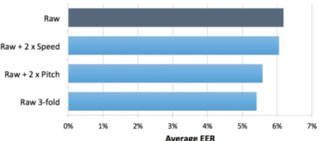
Figure 1: Average EER when evaluating the addition of pitch and speed variation to raw signals during DNN training.
are a major part of this process [6]. We consider the re-quirements of degraded data in this section.
4.1. Equal Treatment of Speakers
Each class (speaker) in network training does not neces-sarily provide equal influence on the training of the em-beddings network. Speakers with segments that are dif-ficult to classify may force the DNN to focus more of its discriminating power on these speakers rather than on other speakers that are easy to classify. To illustrate this, we trained an embeddings DNN on (1) the PRISM train-ing data (includtrain-ing original degradations on a subset of a close-talking microphone), (2) just the raw, non-degraded data from the PRISM training lists, and (3) the raw au-dio from the PRISM lists with one additional degrada-tion copy with noise. We observed that the non-degraded PRISM lists (2) provided a better DNN than the original PRISM lists (1) by 13% relative. We believe this find-ing is due to the use of only a small subset of speak-ers (210 of 3296) having artificially corrupt data during DNN training, forcing the DNN to focus on resolving the issues associated with this corrupt data for speaker clas-sification, and thus being biased to this subset of speakers containing difficult audio. In contrast, adding only a sin-gle copy of each audio file with a random noise signal at 5 db SNR with set (3) provided a significant 25% relative gain in average EER across the benchmarking datasets. This exemplifies the importance of degradations in DNN training as well as maintaining speaker balance across the degraded conditions, so as to reduce the likelihood of ei-ther speaker bias in the DNN, or having the DNN focus on a particular subset of conditions.
4.2. Speed and Pitch Degradation
While prior work has shown the benefit of extrinsic degradations [6] and this is something we extend on in this work, the impact on simulated intrinsic speaker vari-ation has not yet been considered. In this section, we an-alyze the impact of two common methods of data modi-fication to elicit intrinsic variability: speed and pitch. For this process, we start with an extractor trained only on the
raw PRISM data, and add two copies of modified data. The first type is speed-modified via sox to be slower or faster than the original audio by a factor in the range of 0.90–0.95 and 1.05–1.10. The second is the reducing or increasing of pitch via sox to -150 to -50 cents and 50 to 150 cents, where 100 cents is a semitone. Each of these degradations made a notable difference to the signal at the extreme parameter values, while still maintaining a natural sound to the speech audio. To ensure a fair com-parison, we also report results when re-using the raw data three times with different audio labels. This has the ef-fect of covering a wider range of the audio content as the Kaldi recipe naturally limits the number of examples ran-domly selected per speaker per iteration (a small subset of the data covered in a full epoch) during training (default of 35).
Results in Figure 1 show that using speed variation as a degradation provides a limited impact on performance over the use of a single copy of the non-degraded raw data. Pitch variation offers better performance than speed variation, but provides no benefit over using an equiva-lent amount of copies of the original raw data. Besides showing that pitch and speed variation do not improve performance of the embeddings DNN, the difference be-tween Raw and Raw 3-fold additionally indicates that when limited data is available, exposure to more of the content may be necessary to ensure sufficient data cover-age during DNN training.
4.3. Assessing Degradation Level and Type
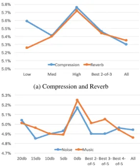
The aim of this section is to observe the effect of different levels of each degradation in order to determine whether a limit exists for each. This was done through combining raw data with a single copy of the data degraded with a specific degradation (such as 5 db SNR music). While the significance of results is hard to gauge given the relatively limited amount of DNN training data, we can observe the following trends in Figure 2:
• Codecs: High compression (low bitrate) provides the worst performance, while combining all codecs is best.
• Reverb: There is a linear relationship between re-verb level and EER. Unlike codecs, the full selec-tion of reverb signals does not outperform using just low-level reverb.
• Noise and Music: Performance improves from 20 db SNR to 5 db SNR, but then quickly degrades at 0 db SNR. This appears to be a cutoff point for train-ing data. Varytrain-ing SNR selection within the best-N-of-5 does not appear to provide a significant differ-ence over using the lowest reasonable SNR of 5 db SNR.
(a) Compression and Reverb
(b) Noise and Music
Figure 2: Average EER when evaluating pools of degra-dations to combine with the raw DNN training data. Only two copies of the data were used in DNN training (raw + degraded from the defined pool). The Best X-of-Y indi-cates expanding the pool for random selection to include the best individual degrees of degradation.
From these trends, diversity in degradation appears to be more important than the degree (i.e., SNR) of the degradation. For this reason, in the remaining experi-ments, we randomly select from all available codecs and fix additive noise to the apparent cutoff point that pro-vides reasonable performance: 5 db SNR. Note that it is, at this point, unclear as to whether high-reverb signals degrade system performance when used in DNN training. Next, we determine the relative importance of each type of degradation. First a DNN baseline was trained using the raw data and four copies of degradations (noise at 5 db SNR, music at 5 db SNR, all codecs, and all re-verb signals). To determine the relative importance of each type of degradation, we trained DNNs each missing one of the degradation types, and also a DNN was trained only on degraded files (no raw included). These DNNs were effectively trained on 80% of the data used in the baseline and are indicated as light blue bars in Figure 3.
Observing the results in Figure 3, we can see that all DNNs trained using the full selection of reverb lev-els are located in the top four bars; they consistently offer the worse performance. The comparison of raw+CMNR and raw+CMN exemplify the fact that using reverb in the current form degrades performance even though more data is being added to the DNN. Based on the trends in Figure 2, we restricted the reverb levels to low reverb only. This provided the best performing system labeled as
Figure 3: Average EER using a leave-one-out approach to DNN training to determine the relative influence of each degradation. The dark bars indicate five-fold train-ing data, while light bars indicate the leave-one-out with codec, music, noise, reverb being indicated by C, M, N, and R, respectively. The keylowRindicates the restric-tion of the reverb pool to low reverb impulse responses only.
raw+CMNlowR. While this tends to contradict the trend in Figure 2 in that ’All’ reverbs provided reasonable per-formance, the current context of pooling multiple degra-dation types is more relevant to the end goal of produc-ing a quality embeddproduc-ings DNN. The conclusion can be drawn, therefore, that the embeddings DNN is quite will-ing to accept a variety of degradations; however, a very low level SNR (i.e., 0 db) degrades performance and sim-ilarly, the embeddings network is sensitive to high levels of reverberation.
5. Data Quantity
Given that artificially degraded data is simple to generate and that the embeddings DNN responds well to degraded data, we now aim to answer two important questions:
• How much degraded data is enough?
• How many speakers are necessary?
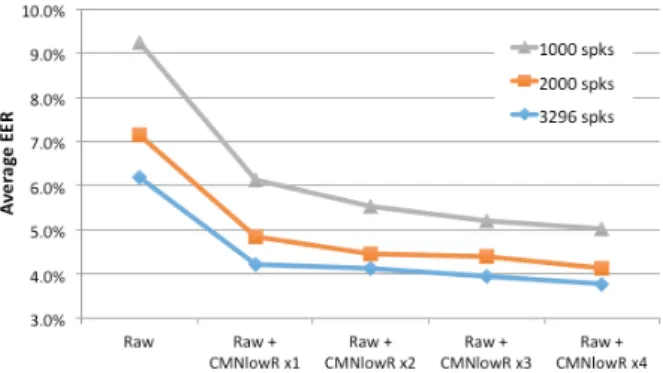
To address these questions, we define three sets of raw data: the full raw PRISM training set consisting of 53,174 segments from 3,296 speakers, and then a ran-dom selection of 2000 and 1000 speakers from this full set, which contained 31,342 and 16,045 segments, re-spectively. From these base sets, we incrementally in-crease the training data through artificial degradations so as to analyze the effect of data quantity for a given num-ber of training speakers. Each new copy of degraded data is drawn randomly from the degradation types using a dif-ferent random seed to result in broader coverage of degra-dation type per original audio file in training. Results are given in Figure 4.
The plot shows that when using only raw data in DNN training, the number of training speakers has a dramatic impact on performance, with performance im-proving 33% when going from 1000 to 3296 speakers.
Figure 4: Average EER when evaluating DNNs trained using 3296, 2000, or 1000 speakers when incrementally adding more copies of degraded data (4-fold each time) during DNN training.
Adding four copies of degraded data (one from each of codec, reverb, noise and music) provides a significant improvement of 32-34% in average EER across the 11 datasets irrespective of the number of speakers in train-ing. As the the amount of degraded data increases (x2-x4), however, the benefit to 1000 speakers can be ob-served to be more apparent than the full speaker set. For instance, moving from 4-fold degradation (x1) to 16-fold (x4), improves the performance 18% relative compared to 10% with the full speaker set. Interestingly, after adding 16 copies of degraded data to the raw data, the downward trend in EER has not ceased.
One consideration here is that the number of epochs is fixed at three in the Kaldi recipe, and the addition of more and more degraded data could in fact be analogous to additional epochs in training (although not entirely, as the extra data provides additional phonetic coverage). To validate that new data was the key contributor and not iterations over a smaller data set, we continued training of the 3296-speaker Raw + CMNlowRx1 DNN in mul-tiples of three epochs. Starting at 4.23%, moving to six epochs reduced the average EER to 4.04%, however ad-ditional epochs failed to improve the network any further. This is in contrast to adding CMNlowRx3 to the raw data, resulting in 3.95%. This trends suggests that increasing the epochs to six and maintaining the use of additional degraded data should allow the network to leverage both methods of improvement.
From the results in Figure 4, we can observe that the degradation from using 2000 speakers instead of 3296 ranges between 9–13%, while reducing to 1000 speakers increases this difference to 24–31%. In conclusion, using at least 2000 speakers and sufficient copies of degraded data appears to provide a reasonable speaker embeddings network.
6. Minibatch Size
It was mentioned in [5] that the GPU memory limited the balance between minibatch size and the maximum num-ber of frames in a training segment, therefore settling at 2-4 seconds per training segments and a minibatch size of 64. We considered this an aspect worthy of note and therefore analyzed the impact of the choice of minibatch size for a DNN trained using a dataset consisting of raw + 1 of each degradation. Using a minibatch size or 64, 128, and 256 resulted in an average EER of 4.35%, 4.29% and 4.34%, respectively. While the variation in performance was limited on the datasets considered in this work, re-sults on several proprietary datasets showed a rather con-sistent improvement when using a minibatch size of 128 as opposed to 64 or 256.
7. Suggested Training Protocol
Numerous aspects of training a speaker embeddings net-work were covered in this study to provide a set of rec-ommendations for those exploring this exciting new tech-nology. In summary, a good speaker embeddings DNN should result by doing the following during training:
1. Using a low SAD threshold, and applying SAD from the raw signal to degraded signals
2. Using as many speakers as is feasible, with a min-imum of 2000 speakers
3. Using a wide variety of degradations, with an SNR of 5 db or higher
4. Not using pitch or speed perturbations 5. Avoiding high levels of reverberation
6. Using as much artificially degraded training data as is feasible
7. Using a 128 minibatch size
8. Training the network with three to six epochs
8. Validation of the Training Protocol
Finally, we aim to validate the suggested training protocol as defined in Section 7. To this end, we leverage the large training set of approximately 5,000 speakers defined in the Kaldi recipe, our own MFCCs and SAD, and com-pare the “baseline“ protocol from [6] to our suggested “improved“ training protocol. Note that we don’t target a minimal pair comparison, but rather validation that the suggested protocol can provide significant improvements over the default recipe.
The raw training data consists of 5,238 speakers from 83,000 audio files. The baseline system increases this data with 128k segments of a degraded version of this
Table 3: Comparison of baseline and improved train-ing protocols based on the default Kaldi traintrain-ing recipe. Metrics reported on SRE’16 and SITW evaluation sets. Domain-adaptation (subscript ‘adp’) performed using mean normalization from the SRE’16 and SITW dev sets.
SITW core SRE’16 Canton. EER DCF10−2 EER DCF10−2 Baseline 6.59% 0.542 7.99% 0.571 Improved 5.75% 0.469 6.35% 0.482 Baselineadp6.13% 0.525 6.76% 0.450
Improvedadp5.33% 0.455 5.16% 0.399
data sourced from MUSAN degradations. These degra-dations include reverb, noise, music and babble and were applied using the Kaldi toolkit. The default minibatch size of 64 and three epochs of training were used. PLDA was learned from SRE’10 data and evaluated on the SRE’16 and SITW datasets. Additionally, to replicate the process in [6], results are reported with a simple form of domain adaptation (denoted with adp) by esti-mating mean-normalization parameters from the SRE’16 dev and SITW dev sets and applying symmetric score normalization [18]. In this work we perform domain adaption and score normalization in a dataset-dependent manner.
The improved system, trained using the suggested protocol, differs in the following ways:
• The degradation pools for noise, reverb, and music were increased by including the degradations used in this article, the codec type was added, and the babble type from Kaldi was removed, as the noise options in our study already incorporated real bab-ble conditions.
• The raw data was degraded 16 times (four copies each for four types of degradation).
• Degradations were applied using the tools used in this work instead of the Kaldi toolkit1.
• A minibatch size of 128 and six epochs of training were used.
In addition to EER, we report performance in terms of the NIST decision cost function (DCF) [19] with a
ptar = 0.01. Results in Table 3 indicate that the
sug-gested embeddings training protocol provides a relative improvement of 13% for both metrics on SITW, and 21%
1In contrast to the Kaldi recipe, we add a single noise signal to each DNN training segment (2-4 seconds) rather than different noises per second (up to five different noises per training segment). The impact of this process has not yet been analyzed, but we believe a single noise sample to sound more naturally occurring.
in EER and 15% in DCF10−2 for the SRE’16 evalua-tion set. It can be seen that the simple form of domain-adaptation and symmetric score normalization further im-proves performance to beyond that of a comparable sys-tem in [6] (label 4.4 in Table 2 of [6] with 6.00% EER for SITW and 5.71% EER for SRE’16 Cantonese).
9. Conclusion
In this study, we focused on the data requirements and sensitivities of a speaker embeddings extractor. The as-pects considered included the impact of speech activ-ity detection, speaker bias in DNN training, degradation types and levels, the amount of training data and number of speakers, and finally the mini-batch size and number of epochs used in DNN training. The network training process showed robustness to SAD threshold selection, and had the ability to leverage diverse artificial degrada-tions with performance continuing to improve after de-grading the raw data 16 times using noise and music at 5 db SNR, compression, and low levels of reverb. In con-trast, sensitivities were demonstrated regarding high re-verberation levels, speaker bias, and noise levels of 0 db SNR or higher. In conclusion, a suggested training proto-col was laid out and validated using a large DNN training set on both SITW and SRE’16 datasets. Future work will consider network structure, calibration aspects of speaker embeddings, and incorporating meta-information directly in the network.
10. References
[1] Y. Lei, N. Scheffer, L. Ferrer, and M. McLaren, “A novel scheme for speaker recognition using a phonetically aware deep neural network,” inProc. ICASSP, 2014.
[2] M. McLaren, Y. Lei, and L. Ferrer, “Advances in deep neural network approaches to speaker recog-nition,” inProc. IEEE ICASSP, 2015.
[3] Ehsan Variani, Xin Lei, Erik McDermott, Ig-nacio Lopez Moreno, and Javier Gonzalez-Dominguez, “Deep neural networks for small foot-print text-dependent speaker verification,” inProc. ICASSP, 2014, pp. 4052–4056.
[4] D. Snyder, P. Ghahremani, D. Povey, D. Garcia-Romero, Y. Carmiel, and Sa Khudanpur, “Deep neural network-based speaker embeddings for end-to-end speaker verification,” in Spoken Language Technology Workshop (SLT). IEEE, 2016, pp. 165– 170.
[5] D. Snyder, D. Garcia-Romero, D. Povey, and S. Khudanpur, “Deep neural network embeddings for text-independent speaker verification,” inProc. Interspeech, 2017, pp. 999–1003.
[6] D. Snyder, D. Garcia-Romero, G. Sell, D. Povey, and S. Khudanpur, “X-vectors: Robust DNN em-beddings for speaker recognition,” inSubmitted to ICASSP, 2018.
[7] NIST SRE 2016 Xvector Recipe, 2017,
https://david-ryan-snyder.github. io/2017/10/04/model_sre16_v2.html. [8] O. Seyed, T. Kheyrkhah, A. Tong, C. Greenberg,
E. Reynolds, L. Mason, and J. Hernandez-Cordero, “The 2016 NIST speaker recognition evaluation,” in
Proc. Interspeech 2017, 2017, pp. 1353–1357. [9] M. McLaren, L. Ferrer, D. Castan, and A. Lawson,
“The speakers in the wild (SITW) speaker recog-nition database,” inProc. Interspeech, 2016, pp. 818–822.
[10] S. Ioffe and C. Szegedy, “Batch normalization: Ac-celerating deep network training by reducing inter-nal covariate shift,” inProc. Int. Conf. on Machine Learning, 2015, pp. 448–456.
[11] L. Ferrer, H. Bratt, L. Burget, H. Cernocky, O. Glembek, M. Graciarena, A. Lawson, Y. Lei, P. Matejka, O. Plchot, and Scheffer N., “Promoting robustness for speaker modeling in the community: The PRISM evaluation set,” in Proc. NIST 2011 Workshop, 2011.
[12] Mitchell McLaren, Victor Abrash, Martin Gracia-rena, Yun Lei, and Jan Pes´an, “Improving robust-ness to compressed speech in speaker recognition.,” inProc. Interspeech, 2013, pp. 3698–3702. [13] J. Ortega-Garcia, J. Gonzalez-Rodriguez, and
V. Marrero-Aguiar, “Ahumada: A large speech cor-pus in spanish for speaker characterization and iden-tification,” Speech communication, vol. 31, no. 2, pp. 255–264, 2000.
[14] GS Morrison, C Zhang, E Enzinger, F Ochoa, D Bleach, M Johnson, BK Folkes, S De Souza, N Cummins, and D Chow, Forensic database of voice recordings of 500+ Australian En-glish speakers, 2015, http://databases. forensic-voice-comparison.net. [15] C Zhang and GS Morrison, Forensic database of
audio recordings of 68 female speakers of Stan-dard Chinese, 2011, http://databases. forensic-voice-comparison.net. [16] K. Walker and S. Strassel, “The RATS radio traffic
collection system,” inProc. Odyssey, 2012. [17] M. McLaren, M. Graciarena, and Y. Lei,
“Soft-Sad: Integrated frame-based speech confidence for speaker recognition,” inProc. ICASSP, 2015, pp. 4694–4698.
[18] Diego Castan, Mitchell McLaren, Luciana Ferrer, Aaron Lawson, and Alicia Lozano-Diez, “Improv-ing robustness of speaker recognition to new condi-tions using unlabeled data,” 2017, pp. 3737–3741. [19] The NIST Year 2012 Speaker
Recogni-tion Evaluation Plan, 2012, http: //www.nist.gov/itl/iad/mig/upload/ NIST_SRE12_evalplan-v17-r1.pdf.