Copulas as High-Dimensional Generative Models:
Vine Copula Autoencoders
Natasa Tagasovska Department of Information Systems
HEC Lausanne, Switzerland [email protected] Damien Ackerer Swissquote Bank Gland, Switzerland [email protected] Thibault Vatter Department of Statistics Columbia University, New York, USA
Abstract
We introduce the vine copula autoencoder (VCAE), a flexible generative model for high-dimensional distributions built in a straightforward three-step procedure. First, an autoencoder (AE) compresses the data into a lower dimensional represen-tation. Second, the multivariate distribution of the encoded data is estimated with vine copulas. Third, a generative model is obtained by combining the estimated distribution with the decoder part of the AE. As such, the proposed approach can transform any already trained AE into a flexible generative model at a low computational cost. This is an advantage over existing generative models such as adversarial networks and variational AEs which can be difficult to train and can impose strong assumptions on the latent space. Experiments on MNIST, Street View House Numbers and Large-Scale CelebFaces Attributes datasets show that VCAEs can achieve competitive results to standard baselines.
1 Introduction
Exploiting the statistical structure of high-dimensional distributions behind audio, images, or video data is at the core of machine learning. Generative models aim not only at creating feature representa-tions, but also at providing means of sampling new realistic data points. Two classes are typically distinguished:explicitandimplicitgenerative models. Explicit generative models make distributional assumptions on the data generative process. For example,variational autoencoders(VAEs) assume that the latent features are independent and normally distributed [37]. Implicit generative models make no statistical assumption but leverage another mechanism to transform noise into realistic data. For example,generative adversarial networks(GANs) use a discriminant model penalizing the loss function of a generative model producing unrealistic data [22]. Interestingly,adversarial autoen-coders(AAEs) combined both features as they use a discriminant model penalizing the loss function of an encoder when the encoded data distribution differs from the prior (Gaussian) distribution [48]. All of these new types of generative models have achieved unprecedent results and also proved to be computationally more efficient than the first generation of deep generative models which require Markov chain Monte Carlo methods [32,30]. However, adversarial approaches require multiple models to be trained, leading to difficulties and computational burden [62,26,24], and variational approaches make (strong) distributional assumptions, potentially detrimental to the generative model performance [64].
We present a novel approach to construct a generative model which is simple, makes no prior distributional assumption (over the input or latent space), and is computationally efficient: thevine copula autoencoders(VCAEs). Our approach, schematized in Figure1combines three tasks. First, an
autoencoder (AE) is trained to provide high-quality embeddings of the data. Second, the multivariate distribution of the encoded train data is estimated with vine copulas, namely, a flexible tool to construct high-dimensional multivariate distributions [3,4,1]. Third, a generative model is obtained by combining the estimated vine copula distribution with the decoder part of the AE.
(2.a) Extract the latent features of X
X Z X’
(3.b) Decode the simulated features
1 2 4 3 5 3, 4 1,2 1, 3 3, 4 3, 5 1, 4 | 2 1, 3 | 2 1,4 | 3 2, 4 | 1, 3 4, 5 | 1, 3 2, 5 | 1, 3, 4 1, 3 1, 2 3, 5 1, 5 | 3 2, 3 | 1 1, 5 | 3 2, 4 | 1, 3 4, 5 | 1, 3
(2.b) Train a vine copula on the latent features
(3.a) Simulate random features from the vine
(1) Train an autoencoder
Vine tree structure
Figure 1: Conceptual illustration of a VCAE. In other words, new data is produced by
decod-ing random samples generated from the vine copula. An already trained AE can thus be trans-formed into a generative model, where the only additional cost would be the estimation of the vine copula. We show in multiple experiments that this approach performs well in building generative models for the MNIST, Large-Scale CelebFaces Attributes, and Street View House Numbers datasets. To the best of our knowledge, this is the first time that vine copulas are used to construct generative models for very high di-mensional data (such as images).
Next, we review the related work most relevant to our setting. The most widespread genera-tive models nowadays focus on synthetic im-age generation, and mainly fall into the GAN or VAE categories, some interesting recent de-velopments include [49,15,26,76,29,14,6]. These modern approaches have been largely in-spired by previous generative models such as belief networks [32], independent component
analysis [33] or denoising AEs [79]. Part of their success can be attributed to the powerful neural network architectures which provide high quality feature representations, often using Convolutional architectures [41]. A completely different framework to model multivariate distributions has been developed in the statistical literature: the so-calledcopulas. Thanks to their ability to capture complex dependence structures, copulas have been applied to a wide range of scientific problems, and their successes have led to continual advances in both theory and open-source software availability. We refer to [56,35] for textbook introductions. More recently, copulas also made their way into machine learning research [43,20,47,78,45,13,74,38]. However, copulas have not yet been employed in constructing high dimensional generative models. While [42,59] use copulas for synthetic data generation, they rely on strong parametric assumptions. In this work, we illustrate hownonparametric vine copulasallow for arbitrary density estimation [50], which in turn can be used to sample realistic synthetic datasets.
Because their training is relatively straightforward, VCAEs have some advantages over GANs. For instance, GANs require some complex modifications of the baseline algorithm in order to avoid mode collapse, whereas vines naturally fit multimodal data. Additionally, while GANs suffer from the “exploding gradients” phenomenon (e.g., see [24]) and require careful monitoring of the training and
early stopping, this is not an issue with VCAEs as they are built upon standard AEs.
To summarize, the contribution of this work is introducing a novel, competitive generative model based on copulas and AEs. There are three main advantages of the proposed approach. First, it offers modeling flexibility by avoiding most distributional assumptions. Second, training and sampling procedures for high-dimensional data are straightforward. Third, it can be used as a plug-in allowing to turn any AE into generative model, simultaneously allowing it to serve other purposes (e.g., denoising, clustering).
The remainder of the paper is as follows. Section2reviews vine copulas as well as their estimation and simulation algorithms. Section3discusses the VCAE approach. Section4presents the results of our experiments. Section5concludes and discusses future research. The supplementary material contains further information on algorithm and experiments, as well as additional experiments.
2 Vine copulas
2.1 Preliminaries and motivation
Acopula, from the latin wordlink, flexibly “couples” marginal distributions into a joint distribution. As such, copulas allow to construct joint distributions with the same margins but different dependence structures, or conversely by fixing the dependence structure and changing the individual behaviors. Thanks to this versatility, there has been an exponentially increasing interest in copula-based models over the last two decades. One important reason lies in the following theorem.
Theorem 1(Sklar’s theorem [71]). The continuous random vectorX = (X1, . . . , Xd)has joint
distributionFand marginal distributionsF1, . . . , Fdif and only if there exist a unique copula1C,
which is the joint distribution ofU= (U1, . . . , Ud) = F1(X1), . . . , Fd(Xd) .
Assuming that all densities exist, we can writef(x1, . . . , xd) = c u1, . . . , ud ⇥Qdk=1fk(xk),
whereui =Fi(xi)andf, c, f1, . . . , fdare the densities corresponding toF, C, F1, . . . , Fd
respec-tively. As such, copulas allow to decompose a joint density into a product between the marginal densitiesfiand the dependence structure represented by the copula densityc.
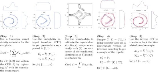
This has an important implication for the estimation and sampling of copula-based marginal distri-butions: algorithms can generally be built into two steps. For instance, estimation is often done by estimating the marginal distributions first, and then using the estimated distributions to construct pseudo-observations via the probability integral transform before estimating the copula density. Similarly, synthetic samples can be obtained by sampling from the copula density first, and then using the inverse probability integral transform to transform the copula sample back to the natural scale of the data. We give a detailed visual example of both the estimation and sampling of (bivariate) copula-based distributions in Figure2. We also refer to Appendix A.1 or the textbooks [56] and [35] for more detailed introductions on copulas.
The availability of higher-dimensional models is rather limited, yet there exists numerous parametric families in the bivariate case. This has inspired the development of hierarchical models, constructed from cascades of bivariate building blocks: thepair-copula constructions(PCCs), also calledvine copulas. Thanks to its flexibility and computational efficiency, this new class of simple yet versatile models has quickly become a hot-topic of multivariate analysis [2].
2.2 Vine copulas construction
Popularized in [3,4,1], PCCs model the joint distribution of a random vector by decomposing the problem into modeling pairs of conditional random variables, making the construction of complex dependencies both flexible and yet tractable. Let us exemplify such constructions using a three dimensional vector of continuously distributed random variablesX = (X1, X2, X3). The joint
densityf ofXcan be decomposed as
f =f1f2f3c1,2c2,3c1,3|2, (1)
where we omitted the arguments for the sake of clarity, andf1, f2, f3are the marginal densities of
X1, X2, X3,c1,2andc2,3are the joint densities of(F1(X1), F2(X2))and(F2(X2), F3(X3)),
c1,3|2is the joint density of(F1|2(X1|X2), F3|2(X3|X2))|X2.
The above decomposition can be generalized to an arbitrary dimensiondand leads to tractable and flexible probabilistic models [34,3,4]. While a decomposition is not unique, it can be organized as a graphical model, a sequence ofd 1nested trees, calledregular vine,R-vine, or simplyvine. Denoting
Tm= (Vm, Em)withVmandEmthe set of nodes and edges of treemform= 1, . . . , d 1, the
sequence is a vine if it satisfies a set of conditions guaranteeing that the decomposition leads to a valid joint density. The corresponding tree sequence is then called thestructureof the PCC and has important implications to design efficient algorithms for the estimation and sampling of such models (see Section2.3and Section2.4).
Each edgeeis associated to a bivariate copula cje,ke|De (a so-calledpair-copula), with the set
De2{1,· · ·, d}and the indicesje, ke2{1,· · ·, d}forming respectively itsconditioning setand
theconditioned set. Finally, the joint copula density can be written as the product of all pair-copula densitiesc=Qdm=11 Qe2Emcje,ke|De. In the following two sections, we discuss two topics that are
important for the application of vines as generative models: estimation and simulation. For further details, we refer to the numerous books and surveys written about them [16,39,72,18,2], as well as Appendix A.2.
2.3 Sequential estimation
To estimate vine copulas, it is common to follow a sequential approach [1,27,50], which we outline below. Assuming that the vine structure is known, the pair-copulas of the first tree, T1, can be
directly estimated from the data. But this is not as straightforward for the other trees, since data from the densitiescje,de|Deare not observed. However, it is possible to sequentially construct
“pseudo-observations” using appropriate data transformations, leading to the following estimation procedure, starting with treeT1: for each edge in the tree, estimate all pairs, construct pseudo-observations for
the next tree, and iterate. The fact that the tree sequenceT1, T2, . . . , Td 1is a regular vine guarantees
that at any step in this procedure, all required pseudo-observations are available. Additionally to Appendix A.2.1 and Appendix A.2.2, we further refer to [1,12,18,19,9,36] for model selection methods and to [17,73,11,27,69] for more details on the inference and computational challenges related to PCCs.
Importantly, vines can be truncated after a given number of trees [12,8,10] by setting pair-copulas in further trees to independence.
Complexity Because there aredpair-copulas inT1,d 1pair-copulas inT2,. . ., and a single
pair-copula inTd 1, the complexity of this algorithm isO(f(n)⇥d⇥truncation level), where
f(n)is the complexity of estimating a single pair and the truncation level is at mostd 1. In our
implementation, described Section2.5,f(n) =O(n). 2.4 Simulation
Additionally to their flexibility, vines are easy to sample from using inverse transform sampling. Let Cbe a copula and U = (U1, . . . , Ud)is a vector of independentU(0,1)random variables.
Then, defineV = (V1, . . . , Vd)through V1 = C 1(U1), V2 = C 1(U2|U1), and so on until
Vd=C 1(Ud|U1, . . . , Ud 1), withC(vk|v1, . . . , vk 1)is the conditional distribution ofVk given
V1, . . . , Vk 1,k = 2, . . . , d. In other words,V is the inverse Rosenblatt transform [65] ofU. It
is then straightforward to notice thatV ⇠C, which can be used to simulate fromC. As for the sequential estimation procedure, it turns out that
• the fact that the tree sequenceT1, T2, . . . , Td 1is a vine guarantees that all the required
conditional bivariate copulas are available (see Algorithm 2.2 of [19]),
• the complexity of the algorithmO(n⇥d⇥truncation level), sincef(n)is trivially the
complexity required for one inversion multiplied by the number of generated samples. Furthermore, there exist analytical expressions or good numerical approximations of such inverses for common parametric copula families. We refer to Section2.5for a discussion of the inverse computations for nonparametric estimators.
2.5 Implementation
To avoid specifying the marginal distributions, we estimate them using a Gaussian kernel with a bandwidth chosen using the direct plug-in methodology of [70]. The observations can then be mapped to the unit square using the probability integral transform (PIT). See steps 1 and 2 of Figure2for an example.
Regarding the copula families used as building blocks for the vine, one can contrast parametric and nonparametric approaches. As is common in machine learning and statistics, the default choice is the Gaussian copula. In Section2.6, we show empirically why this assumption (allowing for dependence between the variables but still in the Gaussian setting) can be too simplistic, resulting in failure to deliver even for three dimensional datasets.
Alternatively, using a nonparametric bivariate copula estimator provides the required flexibility. However, the bivariate Gaussian kernel estimator, targeted at densities of unbounded support, cannot be directly applied to pair-copulas, which are supported in the unit square. To get around this issue, the trick is to transform the data to standard normal margins before using a bivariate Gaussian
kernel. Bivariate copulas are thus estimated nonparametrically using the transformation estimator [67,47,50,21] defined as b c(u, v) = 1 n n X j=1 N( 1(u), 1(v)| 1(u j), 1(vj),⌃) ( 1(u)) ( 1(v)) , (2)
whereN(·,·| 1, 2,⌃)is a two-dimensional Gaussian density with mean 1, 2,and covariance
matrix⌃=n 1/3Cor( 1(U), 1(V)). For the notation we let , and 1to be the standard
Gaussian density, distribution and quantile function respectively. See step 3 of Figure2for an example.
Figure 2: Estimation and sampling algorithm for a pair copula.
Along with vines-related functions (i.e., for sequential estimation and simulation), the Gaussian copula and (2) are implemented in C++ as part ofvinecopulib[51], a header-only C++ library for copula models based onEigen[25] andBoost[68]. In the following experiments, we use the R interface [61] interface tovinecopulibcalledrvinecopulib[53], which also includekde1d[52] for univariate density estimation.
Note that inverses of partial derivatives of the copula distribution corresponding to (2) are required to sample from a vine, as described in Section2.4. Internally,vinecopulibconstructs and stores a grid over[0,1]2along with the evaluated density at the grid points. Then, bilinear interpolation
is used to efficiently compute the copula distributionCb(u, v)and its partial derivatives. Finally,
vinecopulibcomputes the inverses by numerically inverting the bilinearly interpolated quantities using a vectorized version of the bisection method, and we show a copula sample example as step 4 of Figure2. The consistency and asymptotic normality of this estimator are derived in [21] under assumptions described in Appendix A.3.
To recover samples on the original scale, the simulated copulas samples, often called pseudo-samples, are then transformed using the inverse PIT, see step 5 of Figure2. In Appendix C.1, we show that this estimator performs well on two toy bivariate datasets that are typically challenging for GANs: a grid of isotropic Gaussians and the swiss roll.
2.6 Vines as generative models
To exemplify the use of vines as generative models, let us consider as a running example a three dimensional datasetX1, X2, X3withX1, X2 ⇠U[ 5,5]andX3 =
p
X2
1+X22+U[ 0.1,0.1].
The joint density can be decomposed as in the right-hand side of (1), and estimated following the procedures described in Section2.5and Section2.3. With the structure and the estimated pair copulas, we can then use vines as generative models.
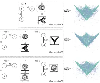
In Figure3, we showcase three models. C1 is a nonparametric vine truncated after the first tree. In other words, it setsc2,3|1to independence. C2 is a nonparametric vine with two trees. C3 is a
Gaussian vine with two trees. On the left panel, we show their vine structure, namely the trees and the pair copulas. On the right panel, we present synthetic samples from each of the models in blue, with the green data points corresponding topX2
1 3 2 Tree 1 Tree 2 1,2 1,3 Vine copula C2 1 3 2 Tree 1 Vine copula C1 2,3|1 1,2 1,3 1,2 1,3 1 3 2 Tree 1 Tree 2 1,2 1,3 Vine copula C3 2,3|1 1,2 1,3 1,3 z 1 z 2 − 3−2−10123 − 3 − 2 − 1 0 1 2 3 1,2 z1 z 2 −3−2−10123 − 3 − 2 − 1 0 1 2 3 1,2 z1 z2 −3−2−10123 −3 −2 −1 0 1 2 3 z1 z2 −3−2−10123 −3 −2 −1 0 1 2 3 1,2 1,3 z1 z2 −3−2−10123 −3 −2 −1 0 1 2 3 z1 z2 −3−2−10123 − 3 − 2 − 1 0 1 2 3 1,3 z1 z2 − 3−2−10123 − 3 − 2 − 1 0 1 2 3 z1 z2 −3−2−10123 − 3 − 2 − 1 0 1 2 3
Figure 3: Simulation with different truncation levels, top to bottom - 1 level truncated vine, 2 levels non-parametric vine, 2 levels Gaussian vine.
Comparing C1 to C2 allows to under-stand the truncation effect: C2, be-ing more flexible (fittbe-ing richer/deeper model), captures better the features of the joint distribution. It can be deduced from the fact that data gen-erated by C2 looks like uniformly spread around the pX2
1+X22
sur-face, while data generated by C1 is spread all around. It should be noted that, in both cases, the nonparametric estimator captures the fact thatX1and
X2 are independent, as can be seen
from the contour densities on the left panel. Regarding C3, it seems clear that Gaussian copulas are not suited to handle this kind of dependencies: for such nonlinearities, the estimated correlations are (close to) zero, as can be seen from the contour densities on the left panel.
With this motivation, the next section is dedicated to extending the vine generative approach to high dimensional data. While vines are theoretically suitable for fitting and sampling in high dimensions, they have been only applied to model a few thousands of variables. The reason is mainly that state-of-the-art implementations were geared towards applications such as climate science and financial risk computations. While software such avinecopulibsatisfies the requirements of such problems, even low-resolution images (e.g.,64⇥64⇥3) are beyond its current capabilities. To address this
challenge, we can rely on the embedded representations provided by neural networks.
3 Vine copula autoencoders
The other building block of the VCAE is anautoencoder(AE) [7,31]. These neural network models typically consist of two parts: anencoderf mapping a datumX from the original spaceX to the latent spaceY, and a decoderg mapping a latent codeY from the latent spaceY to the original spaceX. The AE is trained to reconstruct the original input with minimal reconstruction loss, that is X0⇡g(f(X)).
However, AEs simply learn the most informative features to minimize the reconstruction loss, and therefore cannot be considered as generative models. In other words, since they do not learn the distributional properties of the latent features [5], they cannot be used to sample new data points. Because of the latent manifold’s complex geometry, attempts using simple distributions (e.g., Gaussian) for the latent space may not provide satisfactory results.
Nonparametric vines naturally fill this gap. After training an AE, we use its encoder component to extract lower dimensional feature representations of the data. Then, we fit a vine without additional restrictions on the latent distribution. With this simple step, we transform AEs into generators, by systematically sampling data from the vine copula, following the procedure from Section2.4. Finally, we use the decoder to transform the samples from vine in latent space into simulated images in pixel space. A schematic representation of this idea is given in Figure1and pseudo-code for the VCAE algorithm can be found in Appendix B.
The vine copula is fitted post-hoc for two reasons. First, since the nonparametric estimator is consistent for (almost) any distribution, the only purpose of the AE is to minimize the reconstruction error. The AE’s latent space is unconstrained and the same AE can be used for both conditional and unconditional sampling. Second, it is unclear how to train a model that includes a nonparametric estimator since it has no parameters, there is no loss function to minimize or gradients to propagate. One possibility would be using spline estimators, which would allow to train the model end-to-end by fitting the basis expansion’s coefficients. However, spline estimators of copula densities have been empirically shown to have inferior performance than the transformation kernel estimator [55].
There is some leeway in modeling choices related to the vine. For instance, the number of trees as well as the choice of copula family (i.e., Gaussian or nonparametric) have an impact of the synthetic samples, as sharper details are expected from more flexible models. Note that one can adjust the characteristics of the vine until an acceptable fit of the latent features even after the AE is trained.
4 Experiments
To evaluate VCAEs as generative models, we follow an experimental setup similar as related works on GANs and VAEs. We compare vanilla VAEs to VCAEs using the same architectures, but replacing the variational part of the VAEs by vines to obtain the VCAEs. From the generative adversarial framework, we compare to DCGAN [62]. The architectures for all networks are described in Appendix D.
Additionally, we explore two modifications of VCAE, (i) Conditional VCAE, that is sampling from a mixture obtained by fitting one vine per class label, and (ii) DEC-VCAE, namely adding a clustering-related penalty as in [81]. The rationale behind the clustering penalty was to better disentangle the features in the latent space. In other words, we obtain latent representations where the different clusters (i.e., classes) are better separated, thereby facilitating their modeling.
4.1 Experimental setup Datasets and metrics
We explore three real-world datasets: two small scale - MNIST [40] and Street View House Numbers (SVNH) [57], and one large scale - CelebA [44]. While it is generally common to evaluate models by comparing their log-likelihood on a test dataset, this criterion is known to be unsuitable to evaluate the quality of sampled images [75]. As a result, we use an evaluation framework recently developed for GANs [82]. According to [82], the most robust metrics for two sample testing are theclassifier two sample test(C2ST, [46]) andmean maximum discrepancyscore (MMD, [23]). Furthermore, [82] proposes to use these metrics not only in the pixel space, but over feature mappings in convolution space. Hence, we also compare generative models in terms of Wasserstein distance, MMD score and C2ST accuracy over ResNet-34 features. Additionally, we also use thecommon inception score [66] andFréchet inception distance(FID, [28]). For all metrics, lower values are better, except for inception. We refer the reader to [82] for further details on the metrics and the implementation. Architectures, hyperparameters, and hardware
For all models, we fix the AE’s architecture as described in Appendix D. Parameters of the optimizers and other hyperparameters are fixed as follows. Unless stated otherwise, all experiments were run with nonparametric vines and truncated after 5 trees. We use deep CNN models for the AEs in all baselines and follow closely DCGAN [62] with batch normalization layers for natural image datasets. For all AE-based methods, we use the Adam optimizer with learning rate 0.005 and weight decay 0.001 for all the natural image experiments, and 0.001 for both parameters on MNIST. For DCGAN, we use the recommended learning rate 0.0002 and 1= 0.5for Adam. The size of the latent spaces
zwas selected depending on the dataset’s size and complexity. For MNIST, we present results with z= 10, SVHNz= 20and for CelebAz= 100. We chose to present the values that gave reasonable results for all baselines. For MNIST, we used batch size of 128, for SVHN 32, and for CelebA batches of 100 samples for training. All models were trained on a separate train set, and evaluated on hold out test sets of 2000 samples, which is the evaluation size used in [82]. We used Pythorch 4.1 [58], and we provide our code in Appendix E. All experiments were executed on an AWS instance p2.xlargewith an NVIDIA K80 GPU, 4 CPUs and 61 GB of RAM.
4.2 Results MNIST
In Figure4, we present results from VCAE to understand how different copula families impact the quality of the samples. The independence copula corresponds to assuming independence between the latent features as in VAEs. And the images generated using nonparametric vines seem to improve over the other two. Within our framework, the training of the AE and the vine fit are independent. And we can leverage this to perform conditional sampling by fitting a different vine for each class of digit. We show results of vine samples per digit class in Figure4.
8 7 6 3 2 1 9 4 0 5 Class label 0 1 2 3 4 5 6 7 8 9 Class label Nonparametric Independent Gaussian
Figure 4: Left - impact of copula family selection onMNIST. Middle and Right - random samples of ConditionalVCAEonMNISTandSVHN.
VAE VCAE DEC-VCAE DCGAN
Figure 5: Left to right, random samples ofVAE,VCAE,DEC-VCAE, andDCGANforSVHN. SVHN
The results in Figure5show that the variants of vine generative models visually provide sharper images than vanilla VAEs when architectures and training hyper-parameters are the same for all models. All AE-based methods were trained on latent spacez = 20for 200 epochs, while for
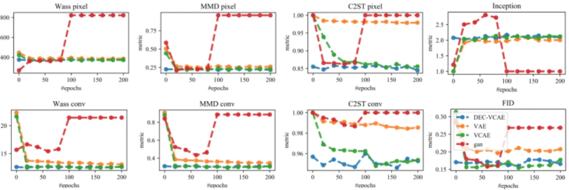
DCGAN we usez= 100and evaluate it at its best performance (50 epochs). In Figure6, we can see
that VCAE and DEC-VCAE have very similar and competitive results to DCGAN (at its best) across all metrics, and both clearly outperform vanila VAE. Finally, the FID score calculated with regards to
104real test samples are has0.205for VAE,0.194for DCGAN and0.167for VCAE which shows
that VCAE also has slight advantage using this metric. In Appendix C.2, Figure12and Figure13 show similar results respectively for the MNIST and CelebA datasets.
Figure 6: Various evaluation scores for all baselines on theSVHNdataset. CelebA
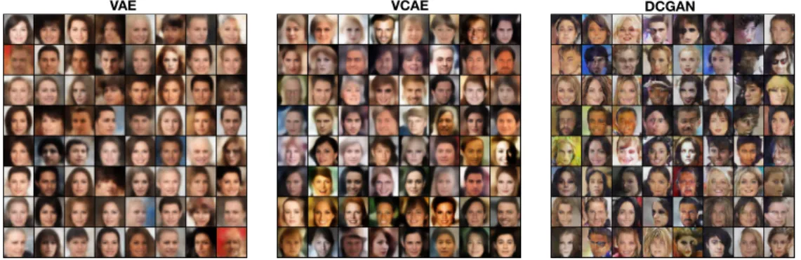
In the large scale setting, we present results for VCAE, VAE, and DCGAN only, because our GPU ran out of memory on DEC-VCAE. From the random samples in Figure7, we see that, for the same amount of training (in terms of epochs), VCAE results is not only sharper but also produce more diverse samples. VAEs improve using additional training, but vine-based solutions achieve better results with less resources and without constraints on the latent space. Note that, in Appendix C.3, we also study the quality of the latent representation.
To see the effect of the number of trees in the vine structure, we include Figure8, where we can see that from the random sample the vine with five trees provides images with sharper details.
VAE VCAE DCGAN
Figure 7: Random samples for models trained on theCelebAdataset, forVAEandVCAEat 200 epochs, and forDCGANbest results at 30 epochs.
5 trees 1 tree
5 trees
1 tree
Figure 8: Higher truncation - sharper images. Since, as stated in Section2.3and Section2.4, the
algorithms complexity increases linearly with the number of trees, we explore the trade-off between computation time and quality of the samples in Ap-pendixC.4. Results show that, as expected, deeper vines, and hence longer computation times, improve the quality of the generated images. Finally, as for SVHN, the FID score shows an advantage of the vine-base method over VAEs as we find 0.247 for VAE and 0.233 for VCAE. For DCGAN the FID score is
0.169 which is better than VCAE, however, looking at the random batch samples in Figure7although GANs outputs sharper images, it is clear that VCAE produces more realistic faces.
Execution times
Table 1: Execution times.
MNIST
(200 epochs) (200 epochs)SVHN (100 epochs)CelebA
VAE 50 min 4h 7 min 7h
VCAE 55 min 1h 32 min 6.5h
DEC VCAE 101 min 2h 35 min /
DCGAN 120 min (40 epochs) 3h 20 min (50 epochs) 5h (30 epochs) We conclude the experimental section with
Ta-ble1comparing execution times. We note that VCAE compares favorably to VAE, which is a “fair” observation given that the architectures are alike. Comparison to DCGAN is more difficult, due to the different nature of the two frameworks (i.e., based respectively on AEs or adversarial).
It should also be noted that the implementation of VCAE is far from optimal for two reasons. First, we use theRinterface tovinecopulibinPythonthroughrpy2. As such, there is a communication overhead resulting from switching betweenRandPython. Second, whilevinecopulibuses native C++11multithreading, it does not run on GPU cores. From our results, this is not problematic, since the execution times are satisfactory. But VCAE could be much faster if nonparametric vines were implemented in a tensor-based framework.
5 Conclusion
In this paper, we present vine copula autoencoders (VCAEs), a first attempt at using copulas as high-dimensional generative models. VCAE leverage the capacities of AEs at providing compressed representations of the data, along with the flexibility of nonparametric vines to model arbitrary probability distributions. We highlight the versatility and power of vines as generative models in high-dimensional settings with experiments on various real datasets. VCAEs results show that they are comparable to existing solutions in terms of sample quality, while at the same time providing straightforward training along more control over flexibility at modeling and exploration (tuning truncation level, selection of copula families/parameter values). Several directions for future work and extensions are being considered. First, we started to experiments with VAEs having flexible distributional assumptions (i.e., by using a vine on the variational distribution). Second, we plan on studying hybrid models using adversarial mechanisms. In related work [38] (see Appendix F), we have also investigated the method’s potential for samplingsequential data(artificial mobility trajectories). There can also be extensions to text data, or investigating which types of vines synthesize best samples for different data types.
References
[1] K. Aas, C. Czado, A. Frigessi, and H. Bakken. Pair-Copula Constructions of Multiple Depen-dence.Insurance: Mathematics and Economics, 44(2):182–198, 2009.
[2] Kjersti Aas. Pair-copula constructions for financial applications: A review. Econometrics, 4(4): 43, October 2016.
[3] Tim Bedford and Roger M. Cooke. Probability Density Decomposition for Conditionally Depen-dent Random Variables Modeled by Vines. Annals of Mathematics and Artificial Intelligence, 32(1-4):245–268, 2001.
[4] Tim Bedford and Roger M. Cooke. Vines – A New Graphical Model for Dependent Random Variables. The Annals of Statistics, 30(4):1031–1068, 2002.
[5] Yoshua Bengio, Aaron Courville, and Pascal Vincent. Representation learning: A review and new perspectives. IEEE transactions on pattern analysis and machine intelligence, 35(8): 1798–1828, 2013.
[6] Diane Bouchacourt, Ryota Tomioka, and Sebastian Nowozin. Multi-level variational autoen-coder: Learning disentangled representations from grouped observations. InAAAI, 2018. [7] Hervé Bourlard and Yves Kamp. Auto-association by multilayer perceptrons and singular value
decomposition.Biological cybernetics, 59(4-5):291–294, 1988.
[8] Eike C. Brechmann and Harry Joe. Parsimonious parameterization of correlation matrices using truncated vines and factor analysis.Computational Statistics and Data Analysis, 77:233–251, 2014.
[9] Eike Christian Brechmann and Claudia Czado. COPAR—multivariate time series modeling using the copula autoregressive model. Applied Stochastic Models in Business and Industry, 31 (4):495–514, 2015.
[10] Eike Christian Brechmann and Harry Joe. Truncation of vine copulas using fit indices. Journal of Multivariate Analysis, 138:19–33, 2015.
[11] Eike Christian Brechmann and Ulf Schepsmeier. Modeling dependence with C-and D-vine copulas: The R-package CDVine. Journal of Statistical Software, 52(3):1–27, 2013.
[12] Eike Christian Brechmann, Claudia Czado, and Kjersti Aas. Truncated regular vines in high dimensions with application to financial data. Canadian Journal of Statistics, 40(1):68–85, March 2012.
[13] Yale Chang, Yi Li, Adam Ding, and Jennifer Dy. A robust-equitable copula dependence measure for feature selection. AISTATS, 2016.
[14] Tatjana Chavdarova and François Fleuret. Sgan: An alternative training of generative adversarial networks. InCVPR, 2018.
[15] Xi Chen, Yan Duan, Rein Houthooft, John Schulman, Ilya Sutskever, and Pieter Abbeel. Infogan: Interpretable representation learning by information maximizing generative adversarial nets. In Advances in neural information processing systems, pages 2172–2180, 2016.
[16] Claudia Czado. Pair-Copula Constructions of Multivariate Copulas. In Piotr Jaworski, Fab-rizio Durante, Wolfgang Karl Härdle, and Tomasz Rychlik, editors,Copula Theory and Its Applications, Lecture Notes in Statistics, pages 93–109. Springer Berlin Heidelberg, 2010. [17] Claudia Czado, Ulf Schepsmeier, and Aleksey Min. Maximum likelihood estimation of mixed
C-vines with application to exchange rates. Statistical Modelling, 12(3):229–255, 2012. [18] Claudia Czado, Eike Christian Brechmann, and Lutz Gruber. Selection of Vine Copulas. In
Piotr Jaworski, Fabrizio Durante, and Wolfgang Karl Härdle, editors,Copulae in Mathematical and Quantitative Finance: Proceedings of the Workshop Held in Cracow, 10-11 July 2012, volume 36. Springer New-York, 2013.
[19] J. Dissmann, Eike Christian Brechmann, Claudia Czado, Dorota Kurowicka, J Dißmann, Eike Christian Brechmann, Claudia Czado, and Dorota Kurowicka. Selecting and estimating regular vine copulae and application to financial returns. Computational Statistics & Data Analysis, 59:52–69, March 2013.
[20] Gal Elidan. Copulas in machine learning. InCopulae in mathematical and quantitative finance, pages 39–60. Springer, 2013.
[21] Gery Geenens, Arthur Charpentier, and Davy Paindaveine. Probit transformation for nonpara-metric kernel estimation of the copula density.Bernoulli, 23(3):1848–1873, 2017.
[22] Ian Goodfellow, Jean Pouget-Abadie, Mehdi Mirza, Bing Xu, David Warde-Farley, Sherjil Ozair, Aaron Courville, and Yoshua Bengio. Generative adversarial nets. InNeurIPS, pages 2672–2680, 2014.
[23] Arthur Gretton, Karsten M Borgwardt, Malte Rasch, Bernhard Schölkopf, and Alex J Smola. A kernel method for the two-sample-problem. InNeurIPS, 2007.
[24] Paulina Grnarova, Kfir Y Levy, Aurelien Lucchi, Nathanael Perraudin, Thomas Hofmann, and Andreas Krause. Evaluating gans via duality. arXiv preprint arXiv:1811.05512, 2018. [25] Gaël Guennebaud, Benoît Jacob, and Others. Eigen v3, 2010.
[26] Ishaan Gulrajani, Faruk Ahmed, Martin Arjovsky, Vincent Dumoulin, and Aaron C Courville. Improved training of wasserstein gans. InNeurIPS, 2017.
[27] Ingrid Hobæk Haff. Parameter estimation for pair-copula constructions. Bernoulli, 19(2): 462–491, 2013.
[28] Martin Heusel, Hubert Ramsauer, Thomas Unterthiner, Bernhard Nessler, and Sepp Hochreiter. Gans trained by a two time-scale update rule converge to a local nash equilibrium. InNeurIPS, 2017.
[29] Irina Higgins, Loic Matthey, Arka Pal, Christopher Burgess, Xavier Glorot, Matthew Botvinick, Shakir Mohamed, and Alexander Lerchner. beta-vae: Learning basic visual concepts with a constrained variational framework.ICLR, 2017.
[30] Geoffrey E Hinton and Ruslan R Salakhutdinov. Reducing the dimensionality of data with neural networks. Science, 313(5786):504–507, 2006.
[31] Geoffrey E Hinton and Richard S Zemel. Autoencoders, minimum description length and helmholtz free energy. InNeurIPS, pages 3–10, 1994.
[32] Geoffrey E Hinton, Simon Osindero, and Yee-Whye Teh. A fast learning algorithm for deep belief nets.Neural computation, 18(7):1527–1554, 2006.
[33] Aapo Hyvärinen and Erkki Oja. Independent component analysis: algorithms and applications. Neural networks, 13(4-5):411–430, 2000.
[34] Harry Joe.Multivariate Models and Dependence Concepts. Chapman & Hall/CRC, 1997. [35] Harry Joe.Dependence modeling with copulas. Chapman and Hall/CRC, 2014.
[36] Matthias Killiches, Daniel Kraus, and Claudia Czado. Model distances for vine copulas in high dimensions. Statistics and Computing, pages 1–19, 2017.
[37] Diederik P Kingma and Max Welling. Auto-encoding variational Bayes. InICLR, 2014. [38] Vaibhav Kulkarni, Natasa Tagasovska, Thibault Vatter, and Benoit Garbinato. Generative
models for simulating mobility trajectories. 2018.
[39] Dorota Kurowicka and Harry Joe.Dependence Modeling. World Scientific Publishing Company, Incorporated, 2010. ISBN 978-981-4299-87-9.
[41] Yann LeCun, Yoshua Bengio, et al. Convolutional networks for images, speech, and time series. The handbook of brain theory and neural networks, 3361(10):1995, 1995.
[42] Haoran Li, Li Xiong, and Xiaoqian Jiang. Differentially Private Synthesization of Multi-Dimensional Data using Copula Functions. InProc. of the 17th International Conference on Extending Database Technology, number c, pages 475–486, 2014.
[43] Han Liu, John Lafferty, and Larry Wasserman. The Nonparanormal: semiparametric estimation of high dimensional undirected graphs.JMLR, 10:2295–2328, 2009.
[44] Ziwei Liu, Ping Luo, Xiaogang Wang, and Xiaoou Tang. Deep learning face attributes in the wild. InICCV, 2015.
[45] David Lopez-Paz.From Dependence to Causation. PhD thesis, University of Cambridge, 2016. [46] David Lopez-Paz and Maxime Oquab. Revisiting classifier two-sample tests. ICLR, 2016. [47] David Lopez-Paz, J M Hernandez-Lobato, and Bernhard Schölkopf. Semi-supervised domain
adaptation with copulas.NeurIPS, 2013.
[48] Alireza Makhzani, Jonathon Shlens, Navdeep Jaitly, and Ian Goodfellow. Adversarial autoen-coders. InICLR, 2016.
[49] Luke Metz, Ben Poole, David Pfau, and Jascha Sohl-Dickstein. Unrolled generative adversarial networks. ICLR, 2016.
[50] Thomas Nagler and Claudia Czado. Evading the curse of dimensionality in nonparametric density estimation with simplified vine copulas. Journal of Multivariate Analysis, 151:69–89, 2016.
[51] Thomas Nagler and Thibault Vatter. vinecopulib: High Performance Algorithms for Vine Copula Modeling in C++, 2017.
[52] Thomas Nagler and Thibault Vatter. kde1d: Univariate Kernel Density Estimation, 2018. R package version 0.2.1.
[53] Thomas Nagler and Thibault Vatter. rvinecopulib: high performance algorithms for vine copula modeling, 2018.
[54] Thomas Nagler, Christian Schellhase, and Claudia Czado. Nonparametric estimation of sim-plified vine copula models: comparison of methods. Dependence Modeling, 5(1):99–120, 2017.
[55] Thomas Nagler, Christian Schellhase, and Claudia Czado. Nonparametric estimation of sim-plified vine copula models: comparison of methods. Dependence Modeling, 5(1):99–120, 2017.
[56] Roger B Nelsen.An introduction to copulas. Springer Science & Business Media, 2007. [57] Yuval Netzer, Tao Wang, Adam Coates, Alessandro Bissacco, Bo Wu, and Andrew Y Ng.
Reading digits in natural images with unsupervised feature learning. InNIPS workshop on deep learning and unsupervised feature learning, volume 2011, page 5, 2011.
[58] Adam Paszke, Sam Gross, Soumith Chintala, Gregory Chanan, Edward Yang, Zachary DeVito, Zeming Lin, Alban Desmaison, Luca Antiga, and Adam Lerer. Automatic differentiation in pytorch. 2017.
[59] Neha Patki, Roy Wedge, and Kalyan Veeramachaneni. The synthetic data vault.Proceedings -3rd IEEE International Conference on Data Science and Advanced Analytics, pages 399–410, 2016.
[60] Robert Clay Prim. Shortest connection networks and some generalizations. The Bell System Technical Journal, 36(6):1389–1401, 1957.
[62] Alec Radford, Luke Metz, and Soumith Chintala. Unsupervised representation learning with deep convolutional generative adversarial networks. ICLR, 2015.
[63] Alfréd Rényi. On measures of dependence. Acta mathematica hungarica, 10(3-4):441–451, 1959.
[64] Danilo Rezende and Shakir Mohamed. Variational inference with normalizing flows. InICML, 2015.
[65] Murray Rosenblatt. Remarks on a multivariate transformation. The annals of mathematical statistics, 23(3):470–472, 1952.
[66] Tim Salimans, Ian Goodfellow, Wojciech Zaremba, Vicki Cheung, Alec Radford, and Xi Chen. Improved techniques for training gans. InNeurIPS, 2016.
[67] Olivier Scaillet, Arthur Charpentier, and Jean-David Fermanian. The estimation of copulas: Theory and practice. Technical report, Ensae-Crest and Katholieke Universiteit Leuven, NP-Paribas and Crest; HEC Geneve and Swiss Finance Institute, 2007.
[68] Boris Schäling.The Boost C++ Libraries. 2011.
[69] Ulf Schepsmeier and Jakob Stöber. Derivatives and Fisher information of bivariate copulas. Statistical Papers, 55(2):525–542, May 2014.
[70] Simon J Sheather and Michael C Jones. A reliable data-based bandwidth selection method for kernel density estimation. Journal of the Royal Statistical Society. Series B (Methodological), pages 683–690, 1991.
[71] A. Sklar. Fonctions de Répartition à n Dimensions et Leurs Marges. Publications de L’Institut de Statistique de L’Université de Paris, 8:229–231, 1959.
[72] Jakob Stöber and Claudia Czado. Sampling Pair Copula Constructions with Applications to Mathematical Finance. In Jan-Frederik Mai and Matthias Scherer, editors,Simulating Copulas: Stochastic Models, Sampling Algorithms and Applications, Series in quantitative finance. World Scientific Publishing Company, Incorporated, 2012.
[73] Jakob Stöber and Ulf Schepsmeier. Estimating standard errors in regular vine copula models. Computational Statistics, 28(6):2679–2707, 2013.
[74] Natasa Tagasovska, Thibault Vatter, and Valérie Chavez-Demoulin. Nonparametric quantile-based causal discovery. arXiv:1801.10579, 2018.
[75] Lucas Theis, Aäron van den Oord, and Matthias Bethge. A note on the evaluation of generative models. InICLR, 2015.
[76] Ilya Tolstikhin, Olivier Bousquet, Sylvain Gelly, and Bernhard Schoelkopf. Wasserstein auto-encoders. ICLR, 2018.
[77] Ilya O Tolstikhin, Sylvain Gelly, Olivier Bousquet, Carl-Johann Simon-Gabriel, and Bernhard Schölkopf. Adagan: Boosting generative models. InNeurIPS, pages 5424–5433, 2017. [78] Dustin Tran, David M Blei, and Edoardo M Airoldi. Copula variational inference. InNeurIPS,
2015.
[79] Pascal Vincent, Hugo Larochelle, Yoshua Bengio, and Pierre-Antoine Manzagol. Extracting and composing robust features with denoising autoencoders. InICML, pages 1096–1103, 2008. [80] Han Xiao, Kashif Rasul, and Roland Vollgraf. Fashion-mnist: a novel image dataset for
benchmarking machine learning algorithms. 2017.
[81] Junyuan Xie, Ross Girshick, and Ali Farhadi. Unsupervised deep embedding for clustering analysis. InICML, 2016.
[82] Qiantong Xu, Gao Huang, Yang Yuan, Chuan Guo, Yu Sun, Felix Wu, and Kilian Weinberger. An empirical study on evaluation metrics of generative adversarial networks. arXiv preprint arXiv:1806.07755, 2018.