University of California, Berkeley
U.C. Berkeley Division of Biostatistics Working Paper Series
Year Paper
Practical Targeted Learning from Large Data
Sets by Survey Sampling
Patrice Bertail
∗Antoine Chambaz
†Emilien Joly
‡∗Modal’X, Universit´e Paris Ouest Nanterre
†Modal’X, Universit´e Paris Ouest Nanterre and Division of Biostatistics, University of
Cali-fornia, Berkeley, [email protected]
‡Modal’X, Universit´e Paris Ouest Nanterre
This working paper is hosted by The Berkeley Electronic Press (bepress) and may not be commer-cially reproduced without the permission of the copyright holder.
http://biostats.bepress.com/ucbbiostat/paper353 Copyright c2016 by the authors.
Practical Targeted Learning from Large Data
Sets by Survey Sampling
Patrice Bertail, Antoine Chambaz, and Emilien Joly
Abstract
We address the practical construction of asymptotic confidence intervals for smooth (i.e., pathwise differentiable), real-valued statistical
parameters by targeted learning from independent and identically distributed data in contexts where sample size is so large that it poses
computational challenges. We observe some summary measure of all data and select a sub-sample from the complete data set by Poisson rejective sampling with unequal inclusion probabilities based on the summary measures. Targeted learn-ing is carried out from the easier to handle sub-sample. We derive a central limit theorem for the targeted minimum loss estimator (TMLE) which enables the con-struction of the confidence intervals. The inclusion probabilities can be optimized to reduce the asymptotic variance of the TMLE. We illustrate the procedure with two examples where the parameters of interest are variable importance measures of an exposure (binary or continuous) on an outcome. We also conduct a simula-tion study and comment on its results.
1
Introduction
Large data sets are ubiquitous nowadays. They pose computational and theoretical challenges. We consider the particular problem of carrying out inference based on semiparametric models by targeted learning [19, 22] from large data sets. We mainly deal with the fact that the sample size N is, say, huge. Even if we also take advantage of easy to handle summary measures of the observations, we do not consider the specific difficulties yielded by the messiness of real big data. This is why we use the expression “large data sets” instead of “big data”.
Confronted with large data sets, many learning algorithms fail to provide an answer in a reasonable time if at all. Following [3], we overcome this computational limitation by (i) selecting n among N observations with unequal probabilities and(ii) adapting targeted learning from this smaller, tamed data set.
Specifically, our objective is to enable the construction of a confidence interval with given asymp-totic level for a statistical parameterψ0 ≡Ψ(P0) based on a sampleO1, . . . , ON of a (huge number)
N of independent and identically distributed (i.i.d.) random variables drawn from P0 ∈ M, where Ψ :M→Rmaps a setMof measures including possible distributions ofO1 to the real line. We focus on the case that the functional Ψ is smooth in the following sense. For every P ∈M, there exists a wide class of one-dimensional paths{Pt:t∈]−c, c[} ⊂Mwith Pt|t=0=P and an influence function D(P)∈L2
0(P) such that, for all |t|< c,
Ψ(Pt) = Ψ(P) + Z D(P)(dPt−dP) +o(t) (1) = Ψ(P) + Z D(P)dPt+o(t). Here, we denoteL2
0(P) the set of centered and square-integrable measurable functions relative to P. Condition (1) trivially holds when Ψ is linear. If, for instance, Ψ is given by Ψ(P) ≡ R
f dP for some measurable function f integrable with respect to (wrt) all elements of M, then (1) holds with D(P) ≡ f −Ψ(P) (without the o-term). Even in the very simple example where f is the identity andM consists of probability measures, hence Ψ(P) =EP[O], it may be computationally difficult, if
not impossible, to build a confidence interval for ψ0 = Ψ(P0) using all observations, merely because it may be very challenging toaccessto all of them in the context of large data sets.
Typical examples of functionals satisfying (1) include pathwise differentiable functionals as intro-duced in [24, Section 25.3]. We will give two examples of such functionals. Pathwise differentiability differs slightly from Gateaux, Hadamard and Fr´echet differentiability. It is one the of key notions in the theory of semiparametric inference.
We overcome the computational hurdle by resorting to survey sampling, specifically to rejective sampling based on Poisson sampling with unequal inclusion probabilities. It is a particular case of sampling without replacement (we refer to [15] for an overview on sampling without replacement). Survey sampling can also rely on the so called sampling entropy [2, 7, 13], but we do not follow this path. Also known as Sampford sampling, rejective Poisson sampling has been thoroughly studied for the last five decades since the publication of the seminal articles [14, 18]. The key object in the analysis
of Sampford sampling is the Horvitz-Thompson (HT) empirical measure. Asymptotic normality of estimators based on the HT empirical measure was first established in [14]. A functional version for the cumulative distribution function was obtained by [26] . Our analysis hinges on the recent study of the HT empirical measure from the viewpoint of empirical processes theory carried out in [3] (we refer the reader to this article for additional references).
For instance [8, 9] show practically how to implement confidence bands for model-assisted es-timators of the mean when the variable of interest is functional and storage capacities are limited (with applications to electricity consumption curves). In that case, survey sampling techniques are interesting alternative to signal compression techniques.
The joint use of survey sampling techniques in conjunction with semiparametric models for in-ference is not new [5, 6]. To the best of our knowledge, however, this is the first attempt to take advantage of survey sampling to enable targeted learning when the data set is so large that computa-tional problems arise. In contrast to naive sub-sampling, sampling designs with unequal probabilities offer a control over the efficiency of estimators. In this light, we propose an alternative to the so called online version of targeted learning [21].
Organization. Section 2 presents our procedure for practical targeted learning from large data sets
by survey sampling and the central limit theorem which enables the construction of confidence inter-vals. Section 3 illustrates Section 2 with two examples, where the parameters of interest are variable importance measures of a (binary or continuous) exposure on an outcome. Section 4 summarizes the results of a simulation study. The proofs are given in appendix.
2
Practical targeted learning
Throughout the article, we denoteµf ≡R
f dµ andkfk2,µ≡(µf2)1/2 for any measureµand function
f (measurable and integrable wrt µ).
2.1 Survey sampling from the large data set and construction of the estimator
Rejective sampling. Letn(N) be a deterministic, user-supplied number of observations to select by
survey sampling. It is a practical, computationally tractable sample size as opposed to the unpractical, hugeN. Because our results are asymptotic we impose that, as N → ∞,
n(N)→ ∞ and n(N) N →0. In the rest of this article, we will simply denoten forn(N).
We employ a specific survey sampling scheme called rejective sampling[14, 3]. The random selec-tion of observaselec-tions from the complete data set can depend on easily accessible summary measures V1, . . . , VN ∈ V attached to O1, . . . , ON. Typically, V1, . . . , VN take finitely many different values or
are low-dimensional, and the implementation of the database is structured/organized based on the values ofV1, . . . , VN.
Lethbe a (measurable) function onV such thath(V)⊂[c(h),∞) for some constantc(h)>0. For each 1≤i≤N, define
pi ≡
nh(Vi)
N . ForN large enough, p1, . . . , pN ∈(0,1). Introduce
• ε1, . . . , εN independently drawn, conditionally on V1, . . . , VN, from the Bernoulli distributions
with parametersp1, . . . , pN, respectively;
• (η1, . . . , ηN) drawn, conditionally onV1, . . . , VN, from the conditional distribution of (ε1, . . . , εN)
given PN
i=1εi =n.
The subset of nobservations randomly selected by rejective sampling is{Oi :ηi = 1,1≤i≤N}.
It is associated with the so-called HT empirical measure defined by
PRp N ≡ 1 N N X i=1 ηi pi Dirac(Oi). (2) Note thatPRp
N is not necessarily a probability measure. However, if h≡1 thenP
p
RN is a probability measure, and rejective sampling is equivalent to selectingnobservations amongO1, . . . , ON uniformly.
For computational reasons, it is not desirable that the event “PN
i=1εi = n” be too unlikely.
Lemma 3.1 in [14] shows that the conditional probability of the event “PN
i=1εi=k” is maximized when k equals the conditional expectation of PN
i=1εi, in which case the conditional probability is
asymp-totically equivalent to (2πPN
i=1pi(1−pi))−1/2. Because the conditional expectation of n−1PNi=1εi
equalsn−1PN
i=1pi=N −1PN
i=1h(Vi), which convergesP0-almost surely toEP0[h(V)], it is thus good practice to choose function h in such a way that EP0[h(V)] be close to 1. When V1, . . . , VN take finitely many different values, it is easy to estimate accurately EP0[h(V)] on an independent sample and, therefore, to adapthso that EP0[h(V)]≈1.
Practical, targeted estimator. Assume that we have constructed Pn∗ ∈M targeted to ψ0 in the
sense that PRp ND(P ∗ n) =oP(1/ √ n). (3)
We defineψ∗n≡Ψ(Pn∗) as our substitution estimator. This construction framesψ∗nin the paradigm of the targeted minimum loss estimation methodology [23, 22].
2.2 Main theorem
Consider a classF of functions mapping a measured space X to R. Set δ > 0 and a semi-metric d
d-balls of radius ε needed to cover F. The corresponding entropy integral for F evaluated at δ is J(δ,F, d)≡Rδ 0 p logN(ε,F, d)dε. LetR:M2 →R be given by R(P, P0)≡Ψ(P0)−Ψ(P)− Z D(P)(dP0−dP) (4)
where the influence functionD(P) is defined before (1). The real numberR(Pn∗, P0) can be interpreted as a second-order term in an expansion ofψn∗ = Ψ(Pn∗) around P0. By (1), we focus on functionals Ψ such that R(P, Pt) =o(t) for a wide class of one-dimensional paths{Pt:t∈]−c, c[} ⊂M such that
Pt|t=0=P. This statement is clarified in the examples of Section 3.
We suppose the existence ofF ⊂ {D(P) :P ∈M}satisfying the three following assumptions:
A1 (complexity) F is separable, for everyf ∈ F,P0f2h−1 <∞, and J(1,F,k · k2,P0)<∞.
A2 (uniform convergence of empirical metric) For every f, f0 ∈ F, if
ρ2N(f, f0)≡ 1 N N X i=1 (f(Oi)−f0(Oi))2 (5)
then, P0-almost surely,
sup f,f0∈F ρN(f, f0) kf −f0k 2,P0 −1 −→ N→∞0.
A3 (first order convergence) With P0-probability tending to 1, D(Pn∗) ∈ F, and there exists
f1 ∈ F such that kD(Pn∗)−f1k2,P0 =oP(1). Moreover, one knows a conservative estimator Σn of σ12 ≡P0f12h−1.
UnderA1, we can define Σ :F2 →
Rgiven by
Σ(f, f0)≡P0f f0h−1. (6) In particular,σ12 inA3equals Σ(f1, f1). An additional assumption is needed:
A4 (second order term) There exists a real-valued random variableγnconverging in probability to
γ1 6= 1 and such thatγn(ψn∗−ψ0) +R(Pn∗, P0) =oP(1/
√
n). Moreover, one knows an estimator Γn such that Γn−γn=oP(1).
We can now state our main theorem.
Theorem 1. Assume that A1, A2, A3 and A4 are met. Then it holds that (1−γn)
√
n(ψ∗n−ψ0)
converges in law to the centered Gaussian distribution with variance σ21. Consequently, for any α ∈
(0,1), " ψ∗n± ξ1−α/2 √ Σn (1−Γn) √ n #
Comments. Assumption A1is typical in semiparametric inference, and should be interpreted as a constraint on the complexity ofF. Theorem 1 relies on the convergence of an empirical process, see Theorem 2. The proof of Theorem 2 uses a chaining argument, and A2 allows to upper-bound the resultingrandomtermJ(δ,F, ρN) by adeterministictermJ(δ,F,k · k2,P0). We say that a classC has finite uniform entropy integral if it admits an envelope functionF and
Z ∞ 0 sup ρ q logN(kFk2,ρ,C,k · k2,ρ)d <∞,
where the supremum is over all probability measures ρ on O such that kFk2,ρ >0. Assumption A2
can be replaced by the alternative
A2* The classF has a finite uniform entropy integral.
VC-classes of uniformly bounded functions satisfy A2* [25, Section 2.6]. Finally, A3 and A4 are technical conditions required by the TMLE procedure. The former is not as mild as one may think at first sight, because the conservative estimation ofσ12 is not trivial. For instance, it is not guaranteed in general that the substitution estimator
Σn≡PRpND(Pn∗)2h
−1
(7) estimates conservatively σ2
1. Relying on the non-parametric bootstrap is not a solution either in general.
We argued thatR(Pn∗, P0) should be interpreted as a second order term. In the simplest examples, this is literally the case and assumingR(Pn∗, P0) =oP(1/
√
n) is natural, see for instance Section 3.1. Sometimes,R(Pn∗, P0) must be corrected by addingγn(ψn∗−ψ0) so that it becomes natural to assume that the corrected expression is oP(1/
√
n), see for instance Section 3.2. Knowing the asymptotic variance of (1−γn)
√
n(ψ∗n−ψ0) allows to discuss further the choice of h. Introduce
f2(V)≡
q
EP0[f1(O)2|V], (8) which satisfiesσ12=P0f12h−1 =P0f22h−1. The Cauchy-Schwarz inequality yields
(P0f2)2 ≤P0f22h−1×P0h=σ12×P0h, (9) and equality occurs whenf2 and hare linearly dependent. Moreover, it should hold that P0h= 1. In view of (9), the optimal h is f2/P0f2, assuming that P0f2 > 0 (otherwise, σ21 = 0). This argument neglects the second-order dependence of γn on h. In practice, we would first sample n0 data using
h0 ≡1, use them to estimatef2 and P0f2 withf2,n0 and Z2,n0, then finally defineh≡f2,n0/Z2,n0 and exclude the sampled data from{O1, . . . , ON}.
The following expansion taken from the proof of Theorem 1 partly explains whyσ21 is the asymp-totic variance of (1−γn)
√
n(ψn∗−ψ0): denoting byP0εthe shared distribution of (O1, ε1), . . . ,(ON, εN),
it holds for anyf inF that
VarPε 0 1 N N X i=1 f(Oi)εi pi ! = 1 NVarP0ε f(O1)ε1 p1
= 1 N EP0 f2(O1) 1 p1 −1 + VarP0(f(O)) .
If, contrary to facts, we could takep1 ≡1 (or, equivalently, n≡N and h≡1), then the asymptotic variance of the resulting TMLE estimator would be of the formN−1VarP0(f(O)) for some limitf, as typically expected. In Section 2.1p1 is chosen in such a way that 1/p1 is typically much larger than 1. Actually, the above RHS expression atf ≡f1 rewrites
1 n P0f12h −1+ n N(P0f1) 2= 1 n σ 2 1+o(1) . (10)
Note the absence of a centering term inP0f12h−1.
3
Two examples
We illustrate Theorem 1 with the inference of two variable importance measures of an exposure, either binary, in Section 3.1, or continuous, in Section 3.2. In both examples, theith observationOi writes
(Wi, Ai, Yi) ∈ O ≡ W × A ×[0,1]. Here, Wi ∈ W is the ith context, Ai ∈ A is the ith exposure
and Yi ∈ [0,1] is the ith outcome. In the binary case, A ≡ {0,1}. In the continuous case, A 3 0
is a bounded subset of R containing 0, which serves as a reference level of exposure. Typically, in
biostatistics or epidemiology, Wi could be the baseline covariate describing the ith subject, Ai could
describe her assignment (e.g., treatment or placebo when A = {0,1} or dose-level when A ⊂R) or exposure (e.g., exposed or not when A = {0,1} or level of exposure when A ⊂ R), and Yi could
quantify her biological response.
3.1 Variable importance measure of a binary exposure In this section,A ≡ {0,1}and ψ0 equals
ψb0≡EP0[EP0[Y|A= 1, W]−EP0[Y|A= 0, W]] (11) (the superscript “b” stands for “binary”). Now, let M be the subset of the set of finite measures on O ≡ W × {0,1} ×[0,1] equipped with the Borel σ-field such that every P ∈ M puts mass on all events of the form B1 × {a} ×B2 (a = 0,1, B1 and B2 Borel sets of W and [0,1]). It contains the set of all possible data-generating distributions for O1 such that the conditional distribution of A given W is not deterministic, including P0. For each P ∈ M, we denote PW, PA|W and PY|A,W
the marginal measure ofW and conditional measures of A and Y given W and (A, W), respectively. (The conditional measurePA|W isP(O) times the conditional law ofAgivenW under the probability
distributionP/P(O). The conditional measurePY|A,W is defined analogously.) We seeψb0as the value atP0 of the functional Ψb characterized overM by
Ψb(P)≡ Z W Z [0,1] y dPY|A=1,W=w(y)−dPY|A=0,W=w(y) ! dPW(w). (12)
In particular, if P is a possible data-generatingdistributionforO1 (i.e., ifP(O) = 1), then Ψb(P) =EP[EP[Y|A= 1, W]−EP [Y|A= 0, W]].
Moreover, under additional causal assumptions, Ψb(P) can be interpreted as the additive causal effect of the exposure on the response, see [17, 22].
Two infinite-dimensional features of every P ∈ M will play an important role in the analysis. Namely, for each P ∈ M and (w, a) ∈ W × A, we introduce and denote gP(0|w) ≡ PA|W=w({0}),
gP(1|w) ≡ PA|W=w({1}), and QP(a, w) ≡
R
[0,1]ydPY|A=a,W=w(y). In particular if P(O) = 1, then gP(1|W) = P(A = 1|W) is the conditional probability that the binary exposure equal one and
QP(A, W) =EP[Y|A, W] is the conditional expectation of the response given exposure and context.
Pathwise differentiability. The functional Ψb is pathwise differentiable at each P ∈ M wrt the
maximal tangent spaceL20(P) (the space of functionss:O →R such that P s= 0 and P s2 <∞) in the following sense [22, Chapter 5 and Section A.3]:
Lemma 1. Fix P ∈M and introduce the influence curveDb(P)∈L20(P) given by Db(P)≡Db1(P) +
Db 2(P) with D1b(P)(O) ≡ QP(1, W)−QP(0, W)−Ψb(P), D2b(P)(O) ≡ (Y −QP(A, W)) 2A−1 gP(A|W) .
For every uniformly boundeds∈L20(P) and every t∈]− ksk−1
∞,ksk−1∞[, define Ps,t ∈M by setting
dPs,t
dP = 1 +ts.
It holds thatt7→Ψb(P
s,t) is differentiable at 0 (as a function fromRtoR) with a derivative at 0 equal toP Db(P)s.
The asymptotic variance of any regular estimator ofΨb(P0) is larger than the Cram´er-Rao
lower-bound P0Db(P0)2. Moreover, for any P, P0 ∈M,
P Db(P0) = Ψb(P)−Ψb(P0) +P(2A−1)(QP0−QP) 1 gP − 1 gP0 . (13)
Consequently if P Db(P0) = 0, then Ψb(P0) = Ψb(P) whenever gP0 =gP or QP0 =QP.
The last statement is called a “double-robustness property”. LetRb :M2→
R be given by
Rb(P, P0)≡Ψb(P0)−Ψb(P)−(P0−P)Db(P), (14) as in (4). In particular,
Rb(P, Ps,t) = Ψb(Ps,t)−Ψb(P)−(Ps,t−P)Db(P)
= Ψb(Ps,t)−Ψb(P)−tP Db(P)s=o(t),
showing that (1) is met.
Furthermore, (13) and P Db(P) = 0 imply
Rb(P, P0) =P0(2A−1)(QP0 −QP) 1 gP0 − 1 gP .
In the context of this example,A4is fulfilled withγn≡0 (hence Γn≡0 andγ1= 0) when Rb(Pn∗, P0) =P0(2A−1)(QP∗ n−QP0) 1 gP∗ n − 1 gP0 =oP(1/ √ n). (15)
Through the product, we will draw advantage of the synergistic convergences ofQP∗
n toQP0 and gPn∗ togP0 (by the Cauchy-Schwarz inequality for example). Note that ifgP0 is known, then we can impose thatgP∗
n =gP0 and R
b(P∗
n, P0) = 0 exactly.
Construction of the targeted estimator. LetQwandGw be two user-supplied classes of functions
mapping A × W to [0,1]. We impose that the elements of Qw are uniformly bounded away from 0
and 1. Similarly, we impose that the elements of Gw are uniformly bounded away from 0. Let ` be
the logistic loss function given by
−`(u, v)≡ulog(v) + (1−u) log(1−v) (allu, v∈[0,1] with conventions log(0) =−∞ and 0 log(0) = 0).
We first estimate QP0 and gP0 with Qn and gn built upon P
p
RN, Q
w and Gw. For instance, one
could simply minimize (weighted) empirical risks and define
Qn ≡ argmin Q∈Qw PRp N`(Y, Q(A, W)) = argmin Q∈Qw N X i=1 ηi pi `(Yi, Q(Ai, Wi)), gn ≡ argmin g∈Gw P p RN`(A, g(A|W)) = argmin g∈Gw N X i=1 ηi pi `(Ai, g(Ai|Wi))
(assuming that the argmins exist). Alternatively, one could prefer minimizing cross-validated (weighted) empirical risks. This is beyond the scope of this article but will be studied in future work. We also estimate the marginal distributionP0,W of W underP0 with
PRp N,W ≡ 1 N N X i=1 ηi pi Dirac(Wi). (16)
LetPn0 be a measure such thatQP0
n =Qn andP 0 n,W =P p RN,W. Then Ψb(Pn0) = 1 N N X i=1 ηi pi (Qn(1, Wi)−Qn(0, Wi)) (17)
is an estimator ofψb0, whose construction is not tailored/targeted toψb0. It is now time to target the inference procedure.
Targeting the inference procedure consists in modifying Pn0 in such a way that the resulting Pn∗ satisfies (3) withDb substituted for D. We first note that, by construction ofPn0,
PRp ND b 1(Pn0) =P p RN,WD b 1(Pn0) = 0.
The construction of Pn∗ based on Pn0 reduces to ensuring PRp ND b 2(Pn∗) = oP(1/ √ n). We achieve this objective by fluctuating the conditional measure ofY given (A, W) only. For this, we introduce the one-dimensional parametric model{Qn(t) :t∈R} given by
logitQn(t)(A, W) = logitQn(A, W) +t
2A−1 gn(A|W)
.
This parametric model fluctuatesQn in the direction of gn2(AA−1|W) in the sense that Qn(0) =Qn and d
dt`(Y, Qn(t)(A, W)) = (Y −Qn(t)(A, W))
2A−1 gn(A|W)
(18) for allt∈R. The optimal move along the fluctuation is indexed by
tn≡arg min t∈R
PRp
N`(Y, Qn(t)(A, W)) (19)
(note that the random functiont7→PRp
N`(Y, Qn(t)(A, W)) is strictly convex).
Define Q∗n ≡ Qn(tn) and let Pn∗ be any element P of M such that QP = Q∗n, gP = gn and
PW =Pn,W0 =P
p
RN,W. Our final estimator is
ψ∗n≡Ψb(Pn∗) = 1 N N X i=1 ηi pi (Q∗n(1, Wi)−Q∗n(0, Wi)).
By definition oftnand (18), we have PRpNDb1(Pn∗) = 0 (just like P
p RND b 1(Pn0) = 0) and PRp N d dt`(Y, Qn(t)(A, W)) t=tn PRp ND b 2(Pn∗) = 0
(whereas it is very unlikely thatPRp ND
b
2(Pn0) be equal to zero). Consequently, (3) is met because
PRp ND
b(P∗
n) = 0.
Theorem 1 is tailored to the present setting in Section 3.3.
3.2 Variable importance measure of a continuous exposure
In this section, A ⊂ R is a bounded subset of R containing 0, which serves as a reference value.
Moreover, we assume that P0,A|W(A= 06 |W) >0 P0,W-almost surely and the existence of a constant
c(P0) > 0 such that P0,A|W(A = 0|W) ≥ c(P0) P0,W-almost surely. Introduced in [12, 10], the true
parameter of interest is ψ0c ≡ arg min β∈R EP0 h (Y −EP0[Y|A= 0, W]−βA) 2i = arg min β∈R EP0 h (EP0[Y|A, W]−EP0[Y|A= 0, W]−βA) 2i (20)
Let M be the set of finite measures P on O ≡ W × A ×[0,1] equipped with the Borel σ-field such that there exists a constant c(P) > 0 guaranteeing that the marginal measure of {w ∈ W : PA|W=w(A \ {0}) > 0 andPA|W=w({0}) ≥c(P)} under PW equals P(O). In particular, P0 ∈ M by
the above assumption.
We see ψ0c as the value atP0 of the functional Ψc characterized overM by Ψc(P)≡arg min
β∈R
Z
A×W
(QP(a, w)−QP(0, w)−βa)2dPA|W=w(a)dPW(w), (21)
using the notation of Section 3.1. By Proposition 1 in [12], for eachP ∈M, Ψc(P) = R A×Wa(QP(a, w)−QP(0, w))dPA|W=w(a)dPW(w) R A×Wa2dPA|W=w(a)dPW(w) . IfP is adistribution, then Ψc(P) = EP[A(QP(A, W)−QP(0, W))] EP[A2] .
For clarity, we introduce some notation. For each P ∈ M and (w, a) ∈ W × A, µP(w) ≡
R AadPA|W=w(a), and gP(0|w) ≡ PA|W=w({0}), ζ2(P) ≡ R Aa2dPA|W=w(a). If P(O) = 1, then µP(W) =EP [A|W],gP(0|W) =P(A= 0|W), and ζ2(P) =EP A2.
Pathwise differentiability. A result similar to Lemma 1 [see 12, Proposition 1] guarantees that Ψc
is pathwise differentiable like Ψb with influence curves Dc(P)≡D1c(P) +D2c(P)∈L20(P), ζ2(P)D1c(P)(O) ≡ A(QP(A, W)−QP(0, W)−AΨc(P)), ζ2(P)D2c(P)(O) ≡ (Y −QP(A, W)) A−µP(W)1{A= 0} gP(0|W) (allP ∈M). LetRc:M2→ R be characterized by Rc(P, P0)≡Ψc(P0)−Ψc(P)−(P0−P)Dc(P).
as in (4) and (14). As in the previous example,Rc satisfies (1) and, for everyP, P0 ∈M,
Rc(P, P0) = 1−ζ 2(P0) ζ2(P) Ψc(P0)−Ψc(P) + 1 ζ2(P)P 0 (QP0(0,·)−QP(0,·)) µP0−µPgP 0(0|·) gP(0|·) . (22) Introduce γn≡1− ζ2(P0) ζ2(P∗ n) and Γn≡1− ζn2(P0) ζ2 n(Pn∗)
whereζn2(P0) andζn2(Pn∗) estimateζ2(P0) andζ2(Pn∗). With these choices, (22) guarantees that A4is
fulfilled in the context of this example whenζ2(Pn∗) converges in probability to a finite real number such thatγ1 6= 1 and
1 ζ2(P∗ n) P0 (QP0(0,·)−QPn∗(0,·)) µP0−µPn∗ gP0(0|·) gP∗ n(0|·) =oP(1/ √ n). Through the product, we will draw advantage of the synergistic convergences ofQP∗
n(0,·) to QP0(0,·) and (µP∗
Construction of the targeted estimator. Let Qw, Mw and Gw be three user-supplied classes
of functions mapping A × W, W and W to [0,1], respectively. We first estimate QP0, µP0 and gP0 withQn and µn and gn built upon PRpN,Qw,Mw and Gw. For instance, one could simply minimize
(weighted) empirical risks and define
Qn ≡ argmin Q∈Qw P p RN`(Y, Q(A, W)) = argmin Q∈Qw N X i=1 ηi pi `(Yi, Q(Ai, Wi)), µn ≡ argmin µ∈Mw PRp N`(A, µ(W)) = argmin µ∈Mw N X i=1 ηi pi `(Ai, µ(Wi)), gn ≡ argmin g∈Gw P p RN`(1{A= 0}, g(0|W)) = argmin g∈Gw N X i=1 ηi pi `(1{Ai = 0}, g(0|Wi))
(assuming that the argmins exist). Alternatively, one could prefer minimizing cross-validated (weighted) empirical risks. We also estimate the marginal distributionP0,W of W under P0 with
PRp N,W ≡ 1 N N X i=1 ηi pi Dirac(Wi), (23)
and the real-valued parameterζ2(P0) with ζ2(PRp
N,X) where P
p
RN,X is defined as in (23) with X and Xi substituted forW andWi.
Let Pn0 be a measure such that QP0
n = Qn, µPn0 = µn, gPn0 = gn, ζ 2(P0 n) = ζ2(P p RN,X), P 0 n,W = PRp
N,W,and from which we can sampleAconditionally onW. Picking up such aP 0
nis an easy technical
task, see [12, Lemma 5] for a computationally efficient choice. Then the initial estimator Ψb(P0
n) of
ψ0b can be computed with high accuracy by Monte-Carlo. It suffices to sample a large numberB (say B = 107) of independent (A(b), W(b)) by (i) sampling W(b) from Pn,W0 = PRp
N,W then (ii) sampling A(b) from the conditional distribution of AgivenW =W(b) underPn0 repeatedly forb= 1, . . . , B and to make the approximation
Ψc(Pn0)≈ B −1PB b=1A(b)(Qn(A(b), W(b))−Qn(0, W(b))) ζ2(P0 n) . (24)
However, the construction Ψc(Pn0) is not tailored/targeted to ψc0 yet. It is now time to target the inference procedure.
Targeting the inference procedure consists in modifying Pn0 in such a way that the resulting Pn∗ satisfies (3) withDcsubstituted forD. We proceed iteratively. Suppose thatPk
n has been constructed
for some k ≥ 0. We fluctuate Pnk with the one-dimensional parametric model {Pnk(t) : t ∈ R, t2 ≤
c(Pnk)/kDc(Pnk)k∞} characterized by
dPnk(t) dPk
n
= 1 +tDc(Pnk). Lemma 1 in [12] shows howQPk
n(t),µPnk(t),gPnk(t),ζ 2(Pk
n(t)) andPn,Wk (t) depart from their counterparts
att= 0. The optimal move along the fluctuation is indexed by tkn≡arg max t PRp Nlog 1 +tDc(Pnk),
i.e., the maximum likelihood estimator oft(note that the random functiont7→PRp
Nlog(1 +tD
c(Pk n))
is strictly concave). It results in the (k+ 1)-th update of P0
n,Pnk+1≡Pnk(tkn).
Contrary to what happened in the first example, see Section 3.1, there is no guarantee that aPnk+1 will coincide with its predecessorPk
n. In this light, the updating procedure in Section 3.1 converged in
one single step. Here, we assume that the iterative updating procedure converges (ink) in the sense that, for kn large enough, PRpND
c(Pkn
n ) = oP(1/
√
n). We set Pn∗ ≡ Pkn
n . It is actually possible to
come up with a one-step updating procedure (i.e., an updating procedure such thatPnk=Pnk+1 for all k≥1) in this example too by relying on so-called universally least favorable models [20]. We adopt this multi-step updating procedure for simplicity.
We can assume without loss of generality that we can sampleAconditionally onW from Pn∗. The final estimator is computed with high accuracy like Ψc(Pn0) previously: withQ∗n≡QP∗
n, we sampleB independent (A(b), W(b)) by(i)samplingW(b)from Pn,W∗ then(ii) samplingA(b) from the conditional distribution ofA given W =W(b) underPn∗ repeatedly for b= 1, . . . , B and make the approximation
ψ∗n≡Ψc(Pn∗)≈ B −1PB b=1A(b)(Q ∗ n(A(b), W(b))−Q∗n(0, W(b))) ζ2(P∗ n) . (25)
Theorem 1 is tailored to the present setting in Section 3.3.
3.3 Tailoring the main theorem in the settings of Sections 3.1 and 3.2 Consider the following assumptions for the study ofψ∗n in the setting of Section 3.1:
A1b The classesQw andGware separable,P
0Q2h−1<∞andP0g2h−1 <∞for all (Q, g)∈ Qw× Gw, and J(1,Qw,k · k
2,P0)<∞,J(1,G
w,k · k
2,P0)<∞. Moreover, A2
∗ is met by Qw and Gw. A2b There exists P1 ∈ M such that kDb(Pn∗)−Db(P1)k2,P0 = oP(1). Moreover, kQ
∗
n−QP0k2,P0 ×
kgn−gP0k2,P0 =oP(1/
√
n) and one knows a conservative estimator Σn ofP0Db(P1)2h−1.
The assumptions required for the study of ψn∗ in the setting of Section 3.2 are very similar:
A1c There exists a setF ⊂ {D(P) :P ∈M}such that A1and A2are verified.
A2c There existζ2
−>0 and P1 ∈M withζ2(P1)≥ζ−2 >0 such that ζ2(Pn∗) =ζ2(P1) +OP(1/ √ n), kDc(Pn∗)−Dc(P1)k2,P0 =oP(1), kQ∗n−QP0k2,P0 ×(kµ ∗ n−µP0k2,P0 +kgn−gP0k2,P0) =oP(1/ √ n).
Moreover, Γn−γn=oP(1) and one knows a conservative estimator Σn of P0Db(P1)2h−1.
In A2b, QP1 and gP1 should be interpreted as the limits of QPn∗ and gPn∗. Likewise, QP1, µP1 and gP1 inA2
cshould be interpreted as the limits of Q P∗
Corollary 1. Set α∈(0,1). In the setting of Section 3.1 and under A1b, A2b, " ψ∗n±ξ1−α/2 √ Σn √ n #
is a confidence interval forψb
0with asymptotic coverage no less than(1−α). In the setting of Section 3.2
and underA1c, A2c, " ψ∗n± ξ1−α/2 √ Σn (1−Γn) √ n #
is a confidence interval forψc0 with asymptotic coverage no less than (1−α).
4
Simulation study
We illustrate the methodology with the inference of the variable importance measure of a continuous exposure presented in Section 3.2. We consider three data-generating distributionsP0,1,P0,2 and P0,3 of a data-structure O = (W, A, Y). The three distributions differ only in terms of the conditional variance of Y given (A, W), but do so drastically. Specifically, O = (W, A, Y) drawn from P0,j
(j= 1,2,3) is such that
• W ≡(V, W1, W2) with P0(V = 1) = 1/6, P(V = 2) = 1/3,P(V = 3) = 1/2 and, conditionally onV, (W1, W2) is a Gaussian random vector with mean (0,0) and variance −01.2−01.2(ifV = 1), (1,1/2) and (0.5 0.1
0.1 0.5) (ifV = 2), (1/2,1) and (1 00 1) (ifV = 3);
• conditionally on W,A= 0 with probability 80% if W1 ≥1.1 and W2 ≥0.8 and 10% otherwise; moreover, conditionally on W and A6= 0,A−1 is drawn from theχ2-distribution with 1 degree of freedom and non-centrality parameter p(W1−1.1)2+ (W2−0.8)2;
• conditionally on (W, A), Y is a Gaussian random variable with mean EP0[Y|A, W]≡A(W1+ W2)/6 +W1+W2/4 + exp((W1+W2)/10) and standard deviation
- 1.5 (ifV = 1), 1 (if V = 2) and 0.5 (if V = 3) forj = 1; - 1 (ifV = 1), 5 (if V = 2) and 10 (ifV = 3) forj= 2; - 50 (if V = 1), 10 (ifV = 2) and 1 (ifV = 3) forj= 3.
The unique true parameter isψ0c= Ψc(P0,1) = Ψc(P0,2) = Ψc(P0,3). It equals approximately 0.1204. ForB = 103 and each j= 1,2,3, we repeat independently the following steps:
1. simulate a data set ofN = 107 independent observations drawn from P0,j;
2. extract n0 ≡103 observations from the data set by survey sampling withh0 ≡1, and based on these observations:
(a) apply the procedure described in Section 3.2 and retrieve Dc(Pkn0
(b) set fn0,1 ≡D
c(Pkn0
n0 ) and regressfn0,1(O)
2 on V, callf
n0,2 the square root of the resulting conditional expectation, see (8);
(c) estimate the marginal distribution ofV, estimateP0fn0,2withπn0,2 and seth≡fn0,2/πn0,2; 3. for eachn in{103,5×103,104,5×104,105}, successively, extract by survey sampling with h a sub-sample ofnobservations from the data set (deprived of the observations extracted in step 2) and, based on these observations, apply the procedure described in Section 3.2. We use Σngiven
in (7) to estimateσ21, although we are not sure in advance that it is a conservative estimator. We thus obtain 15×B estimates ofψ0c and their respective confidence intervals.
To give an idea of what is the optimalh in each case, we save the result of step 2 in the above list in the first of theB simulations under P0,1,P0,2 and P0,3. So, the optimal h equals approximately
- h1 given by (h1(1), h1(2), h1(3))≈(1.03,0.67,1.21) under P0,1; - h2 given by (h2(1), h2(2), h2(3))≈(0.30,0.60,1.50) under P0,2; - h3 given by (h3(1), h3(2), h3(3))≈(4.66,0.53,0.09) under P0,3
Note how different areh1,h2 andh3 (to facilitate the comparisons,h1,h2 andh3 are renormalized to satisfyP0,jhj = 1 for j= 1,2,3).
Applying the TMLE procedure is straightforward thanks to theRpackage calledtmle.npvi[11, 10]. Note, however, that it is necessary to compute Γn and Σn. Specifically, we fine-tune the TMLE
procedure by setting iter (the maximum number of iterations of the targeting step) to 7 and
stoppingCriteriatolist(mic=0.01, div=0.01, psi=0.05). Moreover, we use the defaultflavor
called "learning", thus notably rely on parametric linear models for the estimation of the infinite-dimensional parametersQP0,µP0 and gP0 and their fluctuation. We refer the interested reader to the package’s manual and vignette for details.
Sampford’s sampling method [18] implements the survey sampling described in Section 2.1. How-ever, when the ratio n/N is close to 0 or 1, this acceptance-rejection algorithm typically takes too much time to succeed. In our setting, this is the case when n/N differs from 10−3. To circumvent that issue, we approximate the survey sampling described in Section 2.1 with a Pareto sampling [see Algorithm 2 in 4, Section 5].
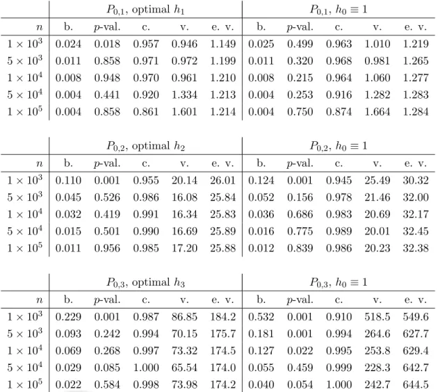
The results are summarized in Table 1. We first focus on the empirical bias of the TMLE and p-values of the Shapiro-Wilk test of normality of its distribution. In all settings, the empirical bias decreases asn grows (underP0,1, the empirical biases for n= 5×10⁴ and n= 105 equal 0.0044 and 0.0036 when relying on h1 or h0). Under each P0,j and for every sub-sample size, the empirical bias
is smaller when relying onhj than on h0, approximately twice smaller under P0,3. As expected due to our choices of conditional standard deviations ofY given (A, W), the empirical bias is larger under P0,3 than underP0,2 and larger underP0,2 than underP0,1. Except underP0,3 when relying onh0, for everyn≥5×10³, thep-values of the Shapiro-Wilk test of normality are coherent with the convergence in law of the TMLE to a Gaussian distribution. Under P0,3 and when relying on h0, there is more
P0,1, optimalh1 P0,1,h0 ≡1 n b. p-val. c. v. e. v. b. p-val. c. v. e. v. 1×10³ 0.024 0.018 0.957 0.946 1.149 0.025 0.499 0.963 1.010 1.219 5×10³ 0.011 0.858 0.971 0.972 1.199 0.011 0.320 0.968 0.981 1.265 1×10⁴ 0.008 0.948 0.970 0.961 1.210 0.008 0.215 0.964 1.060 1.277 5×10⁴ 0.004 0.441 0.920 1.334 1.213 0.004 0.253 0.916 1.282 1.283 1×10⁵ 0.004 0.858 0.861 1.601 1.214 0.004 0.750 0.874 1.664 1.284 P0,2, optimalh2 P0,2,h0 ≡1 n b. p-val. c. v. e. v. b. p-val. c. v. e. v. 1×10³ 0.110 0.001 0.955 20.14 26.01 0.124 0.001 0.945 25.49 30.32 5×10³ 0.045 0.526 0.986 16.08 25.84 0.052 0.156 0.978 21.46 32.00 1×10⁴ 0.032 0.419 0.991 16.34 25.83 0.036 0.686 0.983 20.69 32.17 5×10⁴ 0.015 0.501 0.990 16.69 25.89 0.016 0.775 0.989 20.01 32.45 1×10⁵ 0.011 0.956 0.985 17.20 25.88 0.012 0.839 0.986 20.23 32.38 P0,3, optimalh3 P0,3,h0 ≡1 n b. p-val. c. v. e. v. b. p-val. c. v. e. v. 1×10³ 0.229 0.001 0.987 86.85 184.2 0.532 0.001 0.910 518.5 549.6 5×10³ 0.093 0.242 0.994 70.15 175.7 0.181 0.001 0.994 264.6 627.7 1×10⁴ 0.069 0.268 0.997 73.32 174.5 0.127 0.022 0.995 253.8 629.4 5×10⁴ 0.029 0.085 1.000 65.54 174.0 0.055 0.459 0.999 228.3 642.7 1×10⁵ 0.022 0.584 0.998 73.98 174.2 0.040 0.054 1.000 242.7 644.5
Table 1: Summarizing the results of the simulation study. The top, middle and bottom tables cor-respond to simulations under P0,1, P0,2 and P0,3. Each of them reports the empirical bias of the estimators (b., B−1PB
b=1|ψ∗n,b−ψ0c|), p-value of a Shapiro-Wilk test of normality (p-val.), empirical coverage of the confidence intervals (c.,B−1PB
b=11{ψ0c∈In,b}),ntimes the empirical variance of the
estimators (v., n[B−1PB
b=1ψ∗2n,b−(B−1
PB
b=1ψn,b∗ )2]) and empirical mean of n times the estimated
variance of the estimators (e. v.,B−1PB
b=1Σn,b), for every sub-sample sizenand for bothh optimal andh=h0 ≡1.
evidence of a departure from a Gaussian distribution. Inspecting the results of the simulations studies reveals that this is mostly due to slightly too heavy tails.
We now focus on the empirical coverage, empirical variance and mean of the estimated variance of the TMLE. Consider the table about the simulation under P0,1 first. For n ∈ {103,5×103,104}, the empirical coverage is satisfying when relying on both h1 and h0. At each of these sub-sample sizes, it does seem that we achieve the conservative estimation ofσ12. However, the empirical coverage deteriorates sharply for n∈ {5×104,105}. It appears that, concomitantly, the empirical variance of the estimators increases strongly. This may be due to the fact that, here,nis not that small compared to N, so that neglecting the second LHS term in (10) is inadequate, so that σ12 is not the limiting variance. In conclusion, note that resorting to the optimal h does not yield much gain in terms of empirical variance of the estimators.
We now turn to the two remaining tables. The first striking feature is that the empirical coverage exceeds largely the nominal coverage of 95%. The comparison of the empirical variance with the mean of the estimated variance reveals that we do achieve the conservative estimation of σ2
1. The second striking feature is that the empirical variance stabilizes fornlarger than 103, contrary to what happens under P0,1. It still holds that n may not be small compared to N. Perhaps this is counterbalanced by the fact that, by increasing starkly the conditional variance ofY given (A, W) under P0,2 and P0,3 relative toP0,1, we makeP0f12h−1, the first LHS term in (10), much larger than the second LHS term n(P0f1)2/N. Finally, resorting to the optimal h yields, both under P0,2 and P0,3, considerable gains in terms of empirical variance of the estimators and in terms of the width of the resulting confidence intervals.
Acknowledgements. The authors acknowledge the support of the French Agence Nationale de la
Recherche (ANR), under grant ANR-13-BS01-0005 (project SPADRO).
A
Proof of Theorem 1
Throughout the proofs, “a.b” means that there exists a universal constantL >0 such thata≤Lb. We start with a central limit theorem for the empirical process (√n(PRp
N−P0)f)f∈F. Its proof is given at the end of this section. Recall that a random processGin`∞(F) is k · k2,P0-equicontinuous if for eachξ >0, there existsδ >0 such that, for allf, f0 ∈ F,kf−f0k2,P0 ≤δimpliesP0(|G(f−f0)|)≤ξ.
Theorem 2. Under A1and A2there exists ak · k2,P0-equicontinuous Gaussian processGh ∈`∞(F)
with covariance operator Σ such that (√n(PRp
N −P0)f)f∈F converges weakly in `
∞(F) towards
Gh. The same result holds with F replaced by{f−f1 :f ∈ F }.
We now turn to the proof of Theorem 1. SincePn∗D(Pn∗) = 0 (by definition, the influence function D(Pn∗) is centered under Pn∗), A4rewrites
R(Pn∗, P0) =ψ0−ψn∗−P0D(Pn∗) =−γn(ψn∗−ψ0) +oP(1/
√
hence (1−γn) √ n(ψ∗n−ψ0) =− √ nP0D(Pn∗) +oP(1).
Moreover, (3) implies that the above equality also yields (1−γn) √ n(ψ∗n−ψ0) = √ n(PRp N −P0)D(P ∗ n) +oP(1) = √n(PRp N −P0)f1+ √ n(PRp N −P0)(D(P ∗ n)−f1) +oP(1).
Theorem 2 implies in particular that √n(PRp
N −P0)f1 converges in law to the centered Gaussian distribution with variance Σ(f1, f1).
Let us prove now that√n(PRp
N −P0)(D(P ∗
n)−f1) =oP(1). This is a consequence of Theorem 2
and the concentration inequality of [25, Corollary 2.2.8].
Letk · k2,Σ be the norm onF given bykfk22,Σ≡Σ(f, f). For every δ >0, introduce
Fδ≡ {f ∈ F :P0(f −f1)2 ≤δ2} ⊂ F. The diameter ofFδ wrtk · k2,Σ is at mostδ/
p c(h). By [25, Corollary 2.2.8], E0 " sup f∈Fδ Gh(f−f1) # . Z δ/ √ c(h) 0 q logN(,Fδ,k · k2,Σ)d . Z δ/ √ c(h) 0 q logN(,F,k · k2,Σ)d. (26) Set arbitrarily α, β >0, and choose δ >0 in such a way that
Z δ/ √ c(h) 0 q logN(,F,k · k2,Σ)d≤αβ. By Markov’s inequality, (26) and choice ofδ, it holds that
P0 sup f∈Fδ Gh(f −f1)≥α ! ≤α−1E0 " sup f∈Fδ Gh(f−f1) # .β. Hence, Theorem 2 implies that, fornlarge enough,
P0 √ n(PRp N−P0)(D(P ∗ n))−f1)≥α ≤2β. (27)
Furthermore, by A3, P0(D(Pn∗) 6∈ Fδ) ≤ β for n large enough. Combining this inequality and (27)
finally yields P0 √ n(PRp N −P0)(D(P ∗ n))−f1)≥α ≤ P0 √ n(PRp N −P0)(D(P ∗ n))−f1)≥α , D(Pn∗))∈ Fδ +P0(D(Pn∗))∈ F/ δ) ≤ P0 sup f∈Fδ √ n(PRp N −P0)(f−f1)≥α ! +P0(D(Pn∗))∈ F/ δ)≤3β
fornlarge enough.
Consequently, (1−γn)(ψ∗n−ψ0) converges in law to the centered Gaussian distribution with variance
Proof of Theorem 2.
The proof relies on results from [14, 1]. For eachf ∈ F, define ZN(f)≡PRpNf and Ghn(f)≡ √ n(PRp N −P0)f = √ n(ZN(f)−P0f).
We first state and prove the following lemma, by using [14, Lemma 4.3 and Theorem 7.1]:
Lemma 2. For every (measurable) real-valued function f on O such that P0f2/h is finite, Ghn(f)
converges in law to the centered Gaussian distribution with varianceσ2(f)≡E
P0
f2(O)h(V)−1
.
Proof of Lemma 2. This is a three-step proof.
Step 1: preliminary. Set arbitrarily a measurable function f : O →R such that P0f2/h is finite and define TN(f)≡ 1 N N X i=1 f(Oi)εi pi .
The only difference betweenTN(f) andZN(f) is the substitution of (ε1, . . . , εN) for (η1, . . . , ηN). Since
(O1, ε1), . . . ,(ON, εN) are independently sampled (from P0ε), it holds thatEPε
0 [TN(f)] =P0f and VarPε 0 (TN(f)) = 1 NVarP0ε f(O1)ε1 p1 = 1 nEP0 f2(O) h(V) − 1 N (P0f) 2 = σ 2(f) n +o(1/n). (28)
Thus,√n(TN(f)−P0f) converges in law to the centered Gaussian distribution with varianceσ2(f). The challenge is now to derive another central limit theorem forZN(f) from this convergence in law.
Step 2: coupling. The rest of the proof mainly hinges on coupling. We may assume without loss of generality that there existU1, . . . , UN independently drawn from the uniform distribution on [0,1]
and independent of (O1, . . . , ON) such that, for each 1 ≤ i ≤ N, εi = 1{Ui ≤ pi}. We now define
`N ≡n/PNi=1pi and, for each 1≤i≤N, εi(`N) = 1{Ui ≤`Npi}. This is the first coupling used in
the proof.
The second coupling is more elaborate. Due to Hajek, it gives rise to two random subsets sK and
sn of {1, . . . , N} that we characterize now, in three successive steps. In the rest of this step of the
proof, we work conditionally onO1, . . . , ON.
1. Drawingsn⊂ {1, . . . , N}:
(a) sample (η01, . . . , ηN0 ) from the conditional distribution of (ε01, . . . , ε0N) given PN
i=1ε0i = n
when ε01, . . . , ε0N are independently drawn from the Bernoulli distributions with parameters `Np1, . . . , `NpN, respectively;
(b) define sn={1≤i≤N :ηi0 = 1} and Dn≡Pi∈sn(1−`Npi) for future use.
We say simply thatsnis drawn from the rejective sampling scheme on{1, . . . , N}with parameter
(`Npi :i∈ {1, . . . , N}) (see Section 2).
2. DrawingK ∈ {1, . . . , N}:
(a) sampleε001, . . . , ε00N independently from the Bernoulli distributions with parameters`Np1, . . . , `NpN, respectively; (b) define K≡PN i=1ε 00 i. 3. DrawingsK:
(a) ifK =n, then set sK ≡sn;
(b) if K > n, then draw sK−n from the rejective sampling scheme on {1, . . . , N} \sn with
parameter ((K−n)`Npi/Dn:i∈ {1, . . . , N} \sn) and setsK ≡sn∪sK−n;
(c) if K < n, then draw sn−K from the rejective sampling scheme on sn with parameter
((K−n)`Npi/Dn:i∈sn) and setsK ≡sn\sn−K.
We denote byS the joint law of (sK, sn). Obviously, S is such thatsK ⊂sn orsn⊂sK S-almost
surely. We denote byPthe law of the Poisson sampling scheme,i.e., the law of {1≤i≤N :ε0i = 1}
from the description of how sn is drawn. LawS is a coupling of the rejective sampling scheme and
an approximation to the Poisson sampling scheme P in the sense of the following corollary of [14,
Lemma 4.3].
Proposition 1 (Hajek). If dN ≡ PNi=1pi(1−pi) goes to infinity as N goes to infinity, then the
marginal distribution ofsK when (sK, sn) is drawn from S converges to Pin total variation.
The condition ondN is met for our choice of (p1, . . . , pN).
Step 3: concluding. Introduce
T`N N (f) ≡ 1 N N X i=1 f(Oi)εi(`N) `Npi , TsK N (f) ≡ X i∈sK f(Oi) pi , Tsn N (f) ≡ X i∈sn f(Oi) pi .
The random variablesZN(f),TN`N(f), TNsK(f) andTNsn(f) satisfy the following properties.
• ZN(f) and TNsn(f) share a common law.
• √n(Tsn
N (f)−T sK
N (f)) =oP(1).
Indeed, it is shown in the proof of [14, Theorem 7.1] that the convergence of dN (defined in
Proposition 1) to infinity implies, conditionally on O1, . . . , ON,
√
n(TsK
N (f)−T sn
N (f)) =oP(1).
The unconditional result readily follows.
• TsK
N (f) and T `N
N (f) have asymptotically the same law, in the sense that the total variation
distance between their laws goes to 0 as N goes to infinity. This is a consequence of Proposition 1.
• √n(T`N
N (f)−TN(f)) =oP(1).
It suffices to show that EPε 0 h
(TN(f)−TN`N(f))2
i
=o(1/n). Observe now that
nEPε 0 T`N N (f)−TN(f) 2 = n NEP0ε " ε1(`N) `N −ε1 2 f(O1)2 p21 # = EPε 0 1 `N −2min(1, `N) `N + 1 f(O1)2 h(V1) .
The strong law of large numbers yields that `N converges to 1 almost surely, which implies
1/`N −2 min(1, `N)/`N + 1 converges to 0 almost surely hence the result by the dominated
convergence theorem. Consequently, Ghn(f) ≡
√
n(ZN(f)−P0f) and
√
n(TN(f)−P0f) have asymptotically the same law. The same arguments are valid when {f −f1 : f ∈ F } is substituted for F. Thus, the proof is complete.
We can now prove Theorem 2. We first note that Lemma 2 implies the asymptotic tightness of the real-valued random variable Ghn(f) for all f ∈ F. Moreover, Lemma 2 and the Cram´er-Wold device
yield the convergence in law of (Ghnf1, . . . ,GhnfM) to (Ghf1, . . . ,GhfM) for all (f1, . . . , fM) ∈ FM.
Indeed, for each (f1, . . . , fM) ∈ FM and any (λ1, . . . , λM) ∈ RM, ¯f ≡ PMm=1λmfm is measurable
and P0f¯2/h is finite hence, by Lemma 2, PMm=1λmGhnfm = Ghn( ¯f) converges in law to Gh( ¯f) =
PM
m=1λmGhnfm. In addition, A1implies that the diameter of F wrt k · k2,P0 is finite. Therefore, by [25, Theorems 1.5.4 and 1.5.7], if for allα, β >0, there existsδ >0 such that
lim sup N→∞ P sup f,f0:kf−f0k 2,P0<δ G h nf −Ghnf 0 > α ! ≤β, (29)
then Theorem 2 is valid.
Set arbitrarily α, β, δ >0 and introduceFδ ≡ {f−f0 :f, f0 ∈ F,kf−f0k2,P0 ≤δ}. It is shown in [16] (see also [1]) that η1, . . . , ηN are negatively associatedin the following sense. For each A1, A2 ⊂
{1, . . . , N} with A1∩A2 =∅ and all (measurable) f :Rd1 →R and g:Rd2 →R (d1 ≡card(A1) and d2 ≡card(A2)), iff andg are increasing in every coordinate, then
Hoeffding’s inequality for negatively associated bounded random variables in [3, Theorem S1.2] guarantees that, conditionally onO1, . . . , ON, for all t >0,
P|Ghn(f)|> t O1, . . . , ON ≤exp − 2t 2 ρ2N(f) . Therefore, a classical chaining argument [25, Corollary 2.2.8, for instance]) yields
E " sup f,f0∈F δ |Ghn(f)−Ghn(f0)| O1, . . . , ON # . Z ∞ 0 p logN(,Fδ, ρN)d. (30)
By A2, there exists a deterministic sequence {aN}N≥1 tending to 0 such that, for all f, g ∈ F, ρN(f, g)≤(1 +aN)ρ(f, g) P0-almost surely. Consequently, for every >0, it holds P0-almost surely
that
N(,Fδ, ρN)≤N(/(1 +aN),Fδ,k · k2,P0).
Plugging the previous upper-bound in (30), taking the expectation, using Markov’s inequality and lettingN go to infinity then give
lim sup N→∞ P sup f,f0∈F δ G h n(f)−Ghn(f0) > α ! . α−1 Z ∞ 0 q logN(,Fδ,k · k2,P0)d . α−1J(δ,F,k · k2,P0).
ByA1, it is possible to chooseδ >0 small enough to ensure that the above RHS expression is smaller thenβ, hence (29) holds.
It only remains to determine the covariance ofGh. By adapting the proof of Lemma 2, it appears
that cov(Gh(f),Gh(f0)) =P0f f0/h= Σ(f, f0) for all f, f0 ∈ F.
B
Tailoring the main theorem in the setting of Section 3.1
Let us show that A1b and A2b imply A1–A4 in the setting of Section 3.1. Since Qw and Gw are
uniformly bounded away from 0 and 1,tn(19) necessarily belongs to a deterministic, compact subset
T of R. Define e Qw ≡ expit logitQ+t2A−1 g(A|W) :Q∈ Qw, g∈ Gw, t∈ T then F ≡ {D(P) :P ∈M s.t. QP ∈Qew, gP ∈ Gw}.
Obviously, D(Pn∗) ∈ F and supf∈Fkfk∞ is finite. Furthermore, because expit is a 1-Lipschitz and logit is Lipschitz on any compact subset of (0,1), it holds that Q,e Qe0 ∈Qew respectively parametrized by (Q, g, t) and (Q0, g0, t0) satisfy
kQe−Qe0k2,P0 .kQ−Q0k2,P0 +kg−g0k2,P0+|t−t0|. Therefore, the finiteness of J(1,Qw,k · k
2,P0), J(1,G
w,k · k
2,P0) and J(1,T,| · |) implies the finiteness ofJ(1,Qew,k · k2,P0). Moreover, the separability ofQw and Gw yields thatQew is also separable.
Furthermore, for every P, P0∈Msuch that Db(P), Db(P0)∈ F, it holds that
kDb(P)−Db(P0)k2,P0 .kQP −QP0k2,P
0 +kgP −gP0k2,P0 +|Ψ
b(P)−Ψb(P0)|. (31) We will prove this at the end of the section. By (31), the separability ofQew andGw implies that ofF. In addition, the finiteness of J(1,Qew,k · k2,P0),J(1,Gw,k · k2,P0), J(1,[0,1],| · |) and (31) imply that J(1,F,k · k2,P0) is finite. We prove likewise based on (31) thatF has a finite uniform entropy integral becauseQw and Gw do. Finally, (15) and A2b imply A3(by Cauchy-Schwarz’s inequality) andA4.
Proof of (31). For any P ∈M, denoteqP(W) =QP(1, W)−QP(0, W). SetP, P0 ∈Mb. It holds that
kD1b(P)−D1b(P0)k2,P0 ≤ kqP −qP0k2,P0 +|Ψ b(P)−Ψb(P0 )|. Moreover, kD2b(P)−D2b(P0)k2,P0 = (Y −qP(W)) 2A−1 gP −(Y −qP0(W))2A −1 gP0 2,P0 ≤ (Y −qP(W))(2A−1) 1 gP − 1 gP0 2,P0 + (qP −qP0)2A −1 gP0(W) 2,P0 .kgP −gP0k2,P 0 +kqP −qP0k2,P0,
where the last inequality relies on the uniform boundedness of (Y −qP(W))(2A−1) and g−1P . The
result follows sincekqP −qP0k2,P
0 ≤2kQ−Q 0k
2,P0.
The same kind of arguments allow to verify thatA1cand A2calso imply A1–A4.
References
[1] A. D. Barbour. Poisson approximation and the Chen-Stein method. Statistical Science, 5(4): 425–427, 1990.
[2] Y. Berger. Rate of convergence to normal distribution for the Horvitz-Thompson estimator.
Journal of Statistical Planning and Inference, 67(2):209–226, 1998.
[3] P. Bertail, E. Chautru, and S. Cl´emen¸con. Empirical processes in survey sampling. Scandinavian Journal of Statistics, October 2016. To appear.
[4] L. Bondesson, I. Traat, and A. Lundqvist. Pareto sampling versus Sampford and conditional Poisson sampling. Scandinavian Journal of Statistics. Theory and Applications, 33(4):699–720, 2006.
[5] N. E. Breslow and J. A. Wellner. Weighted likelihood for semiparametric models and two-phase stratified samples, with application to Cox regression. Scandinavian Journal of Statistics, 34(1): 86–102, 2007.
[6] N. E. Breslow and J. A. Wellner. A Z-theorem with estimated nuisance parameters and correction note for “Weighted likelihood for semiparametric models and two-phase stratified samples, with application to Cox regression”. Scandinavian Journal of Statistics, 35, 2008.
[7] K. R. W. Brewer and M. E. Donadio. The high entropy variance of the Horvitz-Thompson estimator. Survey Methodology, 29(2):189–196, 2003.
[8] H. Cardot, D. Degras, and E. Josserand. Confidence bands for Horvitz–Thompson estimators using sampled noisy functional data. Bernoulli, 19(5A):2067–2097, 2013.
[9] H. Cardot, A. Dessertaine, C. Goga, E. Josserand, and P. Lardin. Comparison of different sample designs and construction of confidence bands to estimate the mean of functional data: An illustration on electricity consumption. Survey Methodology/Techniques d’enquˆetes, 39:283–301, 2013.
[10] A. Chambaz and P. Neuvial. tmle.npvi: targeted, integrative search of associations between DNA copy number and gene expression, accounting for DNA methylation. Bioinformatics, 31 (18):3054–3056, 2015.
[11] A. Chambaz and P. Neuvial.Targeted Learning of a Non-Parametric Variable Importance Measure of a Continuous Exposure, 2016. URL http://CRAN.R-project.org/package=tmle.npvi. R package version 0.10.0.
[12] A. Chambaz, P. Neuvial, and M. J. van der Laan. Estimation of a non-parametric variable importance measure of a continuous exposure. Electronic Journal of Statistics, 6:1059–1099, 2012.
[13] A. Grafstr¨om. Entropy of unequal probability sampling designs. Statistical Methodology, 7(2): 84–97, 2010.
[14] J. Hajek. Asymptotic theory of rejective sampling with varying probabilities from a finite popu-lation. The Annals of Mathematical Statistics, 35(4):1491–1523, 12 1964.
[15] M. Hanif and K. R. W. Brewer. Sampling with unequal probabilities without replacement: a review. International Statistical Review/Revue Internationale de Statistique, pages 317–335, 1980.
[16] K. Joag-Dev and F. Proschan. Negative association of random variables with applications. The Annals of Statistics, 11(1):286–295, 03 1983.
[17] J. Pearl. Causality: models, reasoning and inference, volume 29. Cambridge University Press, 2000.
[18] M. R. Sampford. On sampling without replacement with unequal probabilities of selection.
Biometrika, 54(3-4):499–513, 1967.
[19] M. J. van der Laan. Statistical inference for variable importance. International Journal of Biostatistics, 2, 2006.
[20] M. J. van der Laan. One-step targeted minimum loss-based estimation based on universal least favorable one-dimensional submodels. International Journal of Biostatistics, 2016. To appear.
[21] M. J. van der Laan and S. D. Lendle. Online targeted learning. Technical Report 330, U.C. Berke-ley Division of Biostatistics, 2014. URLhttp://biostats.bepress.com/ucbbiostat/paper330. [22] M. J. van der Laan and S. Rose. Targeted learning. Springer, 2011. ISBN 978-1-4419-9781-4.
[23] M. J. van der Laan and D. Rubin. Targeted maximum likelihood learning. International Journal of Biostatistics, 2:Art. 11, 40, 2006. doi: 10.2202/1557-4679.1043.
[24] A. W. van der Vaart. Asymptotic statistics, volume 3 of Cambridge Series in Statistical and Probabilistic Mathematics. Cambridge University Press, Cambridge, 1998.
[25] A. W. van Der Vaart and J. A. Wellner. Weak Convergence and empirical processes. Springer, 1996.
[26] J. C. Wang. Sample distribution function based goodness-of-fit test for complex surveys. Com-putational Statistics & Data Analysis, 56(3):664–679, 2012.