Data parallel algebraic multigrid

(1)

c

(2)

DATA PARALLEL ALGEBRAIC MULTIGRID

BY

STEVEN T DALTON

DISSERTATION

Submitted in partial fulfillment of the requirements

for the degree of Doctor of Philosophy in Computer Science

in the Graduate College of the

University of Illinois at Urbana-Champaign, 2014

Urbana, Illinois

Doctoral Committee:

Professor Luke Olson, Chair

Professor William Gropp

Professor Michael Heath

(3)

Abstract

Algebraic multigrid methods for large, sparse linear systems are central to many computational simula-tions. Parallel algorithms for such solvers are generally decomposed into coarse-grain tasks suitable for distributed computers with traditional processing cores. Accelerating multigrid methods on massively par-allel throughput-oriented processors, on the other hand, demands algorithms with abundant fine-grained parallelism. In this dissertation we analyze and decompose the smoothed aggregation algebraic multigrid method into parallel primitives effectively mapped to emerging architectures. Our formulation is performed in two phases, the first building on high-level generic abstractions to construct our solver in a architecture agnostic manner. Though effective we show that performance is severely limited by irregular sparse ma-trix operations, most notably sparse mama-trix-mama-trix multiplication. In the second phase, we address this performance bottleneck using novel techniques to optimize irregular sparse matrix operations.

This dissertation is also concerned with irregular graph operations necessary to partition sparse matrices into disjoint sets for parallel processing. We apply our solver to accelerate eigenvector computations necessary during spectral partitioning methods and find that performance is limited by multigrid construction. We propose and analyze a novel strategy to accelerate graph Laplacian eigenvector computations by combining iterative methods, namely blocked Lanczos, with breadth first search operations on graphs. By basing our partitioner on primitives with substantial parallelism we demonstrate notable performance improvement compared with generic eigensolvers.

(4)

To my loving wife, Kymberly, for all of her support and encouragement throughout this entire process and my precious son Colin, my future children, grandchildren and great-grandchildren, I dedicate this thesis to

(5)

Acknowledgments

I am grateful for all the friends and family members who have influenced, encouraged, and supported me throughout my entire college career as an undergraduate and graduate student.

• To my advisor, Professor Luke Olson, who introduced me to algebraic multigrid, encouraged my curiosity, and continually provided constructive feedback on my progress throughout this long journey from start to finish for five years, thank you so much for you support and guidance. I know I did not make this process particularly easy at times! This dissertation would not have been possible with anyone else.

• My unofficial co-advisor Nathan Bell, who taught me a great deal on algebraic multigrid, writing programs, writing papers, and many other areas. It is impossible to express how much of an impact working with you had on my graduate experience and my life.

• Michael Heath for encouraging me to attend UIUC during visit day and for serving as my mentor for my first year of graduate school. I thank you for listening to me and giving me sound advice when all I wanted to do was quit.

• Michael Garland for allowing me to spend two productive summers working in his research group at Nvidia and supporting my education with a fellowship. I gained significantly by interacting with members of your group, Duane Merrill, Sean Baxter, Bryan Catanzaro, and Jared Hoberock.

• My friends in scientific computing group – Elena Caraba, Jehanzeb Chaudhry, James Lai, Russ Hewett, Amanda Bienz, Hormozd Gahvari, Mitya Yershov, Matt Wrobel, and Matthew Michelotti - for sharing the graduate school experience with me. I would especially like to thank my qualifying exam study buddy Kaushik Kalyanaraman for spending weeks with me discussing numerical methods in painstaking detail.

• My undergraduate advisor Professor Umakishore Ramachandran at Georgia Tech for nurturing my ideas and allowing me to feel like a contributing member of his research group. Professor George Riley

(6)

for exposing me to my first real research project that set the course for my career. David Smith for supporting my undergraduate education with endless teaching assistantships and witty conversation. • My parents for all of their support both mentally and financially. There is no possible way I would

have made it without the both of you. My brother for being my first research collaborator and mentor as we discovered everything we could about computers together as kids.

• Last but not least my loving wife Kym whose constant love and support throughout this process has been the driving force towards the completion of my graduate studies and this dissertation. My son, Colin, thank you for supplying me with daily inspiration and staying up late to help me write large parts of this dissertation, although I had to remove many of your contributions, since you are still learning to read and write, I will always cherish your enthusiasm and creativity.

(7)

Chapter 1

Introduction

Computational science utilizes computers and mathematics to enhance scientific discovery. This interplay has led to accelerated advancements in a variety of disciplines throughout science. Contributing to this, numerical simulations that were beyond the reach of supercomputers 30 years ago are routinely performed on a single desktop today. This rapid growth in computational power is due to considerable advancements in both computer engineering and algorithmic efficiency. The dependency of the latter property on the former means that architectural shifts necessarily influence the evolution of algorithms and vice versa. In this work we consider specifically numerical algorithms used to solve large systems of linear equations and highlight that emerging highly parallel architectures require the reformulation of computationally optimal numerical solvers.

The motivation for optimal numerical solvers is driven by the demand for increasingly accurate compu-tational models to simulate real world processes. As the fidelity and complexity of these models increases so to does the role of these models in science. Indeed, the ability to predict and analyze physical phe-nomenon based solely on computational data has been solidified as the third modern pillar of the scientific method. Though increased model detail yields more accurate simulations the increased complexity neces-sitates additional degrees of freedom or variables,N, to fully describe the fine-grained processes governing the corresponding system of linear equations, A ∈ RN×N_{. Therefore the cost of computing} _x_given _b _in

Ax=b is heavily dependent on the selected solver and may be unreasonably expensive for direct methods, such as Gaussian elimination which scale asO(N3_{) in both spatial and computational complexity, as shown} in Figure 1.1. The ideal complexity would depend only linearly onN, meaning the cost of computing the solution is proportional to the number of unknowns, which is asymptotically optimal. In turn, the availabil-ity ofO(N) solvers motivates the development of more detailed models creating a circular dependence that pushes the boundaries of both computing and algorithmic capabilities.

The overhead associated with direct methods, in terms of space and computation, is reduced significantly by adopting a strategy based on iterative improvement. A well-known class of theseiterativesolvers is based on Krylov subspaces and includes the conjugate gradient (CG) and generalized minimum residual (GMRES)

(9)

Increased model accuracy Optimal numerical methods (O(N)) Larger sparse system of equations (N) Number of elements Computational w ork p er variable O(N3₎ _O₍_N2₎ _O₍_N_log_N₎ O(N1.5₎ O(N1.2₎ O(N)

Figure 1.1: Improved model accuracy increases the number of unknowns, N, in the resulting linear system which in turn places additional pressure on numerical methods to minimize the costs,O(N), of computing the solution. AsN grows classical approaches that require quadratic or cubic work are no longer feasible.

methods. Krylov methods begin with an initial subspace, usually a single vector, and proceed by repeatedly minimizing some quantity-of-interest over a subspace. The total work required to compute the solution to a prescribed level of accuracy therefore relies heavily on the ability of the method to adequately reduce the error, the difference between the current approximation and true solution, during each iteration. More precisely the convergence is often related to the spectral distribution of the eigenvalues and the modulus of the largest and smallest generally grows withN. Operators with a large disparity in eigenvalues are termed poorly conditioned and consequently require a large number of iterations to converge, which ultimately reduces the algorithmic advantages of these methods.

To address this limitation iterative methods are coupled with preconditioners to improve the operator spectrum and therefore the conditioning. Preconditioners based on multilevel methods are common since they target computing the solution in optimalO(N) complexity. The central idea of multigrid is the hierarchical representation and solution of the original problem at various granularities. Although numerous formulations exist they are broadly grouped into two distinct families: geometric and algebraic. Geometric multigrid (GMG) methods were the earliest approach and generate coarse representations by exploiting the geometric regularity of structured problems. Although GMG is highly effective for many problems, the reliance on structure and geometry limits the general applicability. To address this limitation algebraic multigrid (AMG) methods reduce the dependence on problem geometry; in AMG coarse representations are determined by applying a set of heuristics directly to the linear system. Decreased knowledge concerning the problem instance places an increased burden on AMG methods in the form of a setup in order to construct a hierarchy of levels and transfer operators between levels. Heuristics to guide construction of an algebraic hierarchy are

(10)

numerous but typically rely on a mixture of algebraic and graph theoretic operations to assess the salient features of the underlying problem.

Although the existence of optimal solvers are interesting the true potential of any computational method is only realized when algorithms are coupled with implementations that utilize a given architecture efficiently. This algorithm-architecture coupling has been challenging since the evolution of modern numerical methods has overlapped with dramatic architectural shifts in computer hardware stemming from performance limi-tations of processor cores. The stagnation of single core performance at the end of twentieth century forced the introduction of additional cores to increase performance ushering in a new era of parallel computing. This performance oriented paradigm shift from vertical, increased clock rates, to horizontal, increased cores per chip, has irrevocably impacted both the performance and development of numerical algorithms.

The departure from sequential processing introduces a significantly more complex set of design decisions to facilitate parallel computing. As illustrated in Figure 1.2 multicore CPUs are the natural extension of their unicore predecessors. A moderate increase in the number of cores per chip decreases the per core cache memory size but the architecture design is fundamentally the same, specifically each core still processes a separate stream of instructions on different data, multiple processor multiple data (MIMD). Though effective for many workloads multicore CPUs do not fully exploit abundant fine-grained data-parallel aspects of some computational workloads. For these workloads the number of operations per datum is small but the volume of data is massive, a typical feature of workloads from graphics rendering, therefore graphics processing units (GPUs) that were originally designed to support graphics rendering were repurposed to allow the execution of generalized data-parallel workloads.

CR CR _CR CR CR Con trol UnitCR _CR CR CR CR CR CR CR CR CR CR CR CR CR CR

Increasing number of cores Decreasing memory per core Regs

+ Entire Cache Hierarchy

(L1 and L2)

Memory per core

Processor core DRAM Bandwidth Regs + L1 Regs

Figure 1.2: Latency oriented architectures utilize large on-chip cache memory to reduce expensive accesses to global DRAM. As the number of cores increases the dedicated private memory per core decreases. Throughput oriented architectures substantially increase the number of cores at the expense of a small amount of private memory per core.

(11)

In contrast to CPUs emerging throughput-oriented processors share a single instruction stream therefore all operations are executed across multiple cores in a single instruction multiple data (SIMD) fashion. An-other important distinction is that each core does not have dedicated cache to reduce the expense of slow global memory accesses, instead the bandwidth to fetch data from global memory is considerably higher. The local memory constraint severely limits the working set size of each core to the number of allocated registers. The repercussion of these architecture differences is the need to redesign algorithms to express substantial parallelism and cooperative processing at exceedingly small granularities, sometimes on the order of individual datum. With respect to previous approaches to AMG the units of computational work are too coarse-grained for direct implementation on GPUs.

In this dissertation we focus on the parallel decomposition of smoothed aggregation based AMG methods to solve sparse linear systems,Ax=b, on GPU architectures. AMG is particularly challenging for modern day architectures because hierarchy construction relies on analyzing structures with irregular and data-driven access patterns. We analyze the performance of the operations during both the construction and iterative cycling phases directly on the GPU. We primarily focus on GPUs for several reasons:

• Many of the operations involved in the setup phase are memory-bound therefore it may be beneficial to take advantage of the much higher peak bandwidth capabilities of GPUs.

• Solve phase performance is dominated by sparse matrix-vector operations which are known to perform better in bandwidth rich environments, such as GPUs. However, performing the setup phase on the CPU followed by transferring data to GPU incurs a substantial performance penalty due to the relatively low bandwidth PCI-express interconnect. By constructing the hierarchy completely on the GPU memory copy operations are reduced significantly.

• The resource constraints of parallel processing on GPUs in many cases requires rethinking traditional CPU algorithms. By studying the algorithmic requirements to perform all operations in a throughput-oriented manner we design our methods to support massive fine-grained parallel processing which follows the general trend in computer architectures.

AMG is particularly challenging for modern day architectures because hierarchical construction relies on analyzing data-structures with irregular and data-driven access patterns. We analyze the performance of performing all operations during both the construction and iterative cycling phases directly on the GPU. Although the most common approach to constructing GPU algorithms begin by decomposing complex al-gorithms into a small set of optimized programs, known as kernels, we propose a decomposition based on parallel primitives that abstracts the architecture agnostic algorithmic specification from the architecture

(12)

specific implementation. The resulting formulation is architecture independent and, although we specifically study the performance implications on GPUs, our formulation extends to any architecture exposing a small set of optimized primitives. We study the performance limiting components of this initial decomposition and subsequently introduce architecture specific optimizations to improve the performance of a small set of key tasks, mainly sparse matrix-sparse matrix computations. The contributions of this dissertation are:

• Decomposition and analysis of AMG methods amenable for fine-grained execution on modern highly parallel architectures;

• Strategies to improve the performance of irregular operations involving sparse matrices through regu-larization of data-dependent irregular workloads;

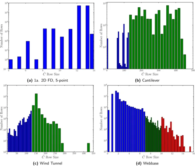
• A systematic methodology to classify, compare, and analyze the multiplication of sparse matrices based on histograms; and

• An efficient approach to partitioning sparse matrices based on coupling breadth-first search (BFS) type methods with spectral partitioning.

In Chapter 2 we describe a parallel decomposition of AMG for GPU architectures using a small set of parallel primitives. Chapter 3 presents an approach to accelerate the performance of sparse matrix operations by combining analysis of the row-wise work of the output matrix with optimized hierarchical sorting routines executing at various levels of parallelism. Chapter 4 introduces a structured scheme to discuss and analyze the performance of row-wise sparse matrix multiplication based on the intermediate work generated. In Chapter 5 we propose and analyze a novel strategy to accelerate spectral graph partitioning by coupling well-understood operations on graphs, BFS with blocked Lanczos methods.

(13)

Chapter 2

Algebraic Multigrid

Multigrid methods precondition large, sparse linear systems of equations and in recent years have become a robust approach for a wide range of problems. One reason for this increased utility is the trend toward more algebraic approaches. In the classical,geometric form of multigrid, the performance relies largely on specialized smoothers, and a hierarchy of grids and interpolation operators that are predefined through the geometry and physics of the problem. In contrast, algebraic-based multigrid methods (AMG) attempt to automatically construct a hierarchy of grids and intergrid transfer operators without explicit knowledge of the underlying problem — i.e., directly from the linear system of equations [71, 82]. Figure 2.1 depicts the contrasting nature of the two hierarchies generated by both approaches.

Ω3 Ω2 Ω1 Ω0 P2 P1 P0 R2 R1 R0 (a)Geometric Ω3 Ω2 Ω1 Ω0 P2 P1 P0 R2 R1 R0 (b)Algebraic

Figure 2.1: Geometric methods construct all components of the multigrid hierarchy based on regularized coarsening strategies. In contrast algebraic methods are able to operate on unstructured discretizations by defining coarse levels algebraically based on matrix and graph operations.

Parallel approaches to multigrid are plentiful. Algebraic multigrid methods have been successfully par-allelized on distributed-memory CPU clusters using MPI [20, 23] and more recently with a combination of

(14)

MPI and OpenMP [3], to better utilize multi-core CPU nodes. While such techniques have demonstrated scalability to large numbers of processors, they are not immediately applicable to the GPU. In particular, ef-fective use of GPUs requires substantialfine-grainedparallelism at all stages of the computation. In contrast, the parallelism exposed by existing methods for distributed-memory clusters of traditional cores is compa-rably coarse-grained and cannot be scaled down to arbitrarily small subdomains. Indeed, coarse-grained parallelization strategies are qualitatively different than fine-grained strategies.

For example, it is possible to construct a successful parallel coarse-grid selection algorithm by partitioning a large problem into sub-domains and applying an effective, serial heuristic to select coarse-grid nodes on the interior of each sub-domain, followed by a less-effective but parallel heuristic to the interfaces between sub-domains [43]. An implicit assumption in this strategy is that the interiors of the partitions (collectively) contain the vast majority of the entire domain, otherwise the serial heuristic has little impact on the output. Although this method is scalable to arbitrarily fine-grained parallelism in principle, the result is qualitatively different. In contrast, the methods we develop do not rely on partitioning and expose parallelism to the finest granularity — i.e., one thread per matrix row or one thread per nonzero entry.

Geometric multigrid methods were the first to be parallelized on GPUs [13, 38, 79]. These “GPGPU” ap-proaches, which preceded the introduction of the CUDA and OpenCL programming interfaces, programmed the GPU through existing graphics application programming interfaces (APIs) such as OpenGL and Di-rect3d. Subsequent works demonstrated GPU-accelerated geometric multigrid for image manipulation [49] and CFD [25] problems. Previous works have implemented the cycling stage of algebraic multigrid on GPUs [36, 41], however hierarchy construction remained on the CPU. A parallel aggregation scheme is described in [80] that is similar to ours based on maximal independent sets, while in [1] the effectiveness of parallel smoothers based on sparse matrix-vector products is demonstrated. Although these works were implemented for distributed CPU clusters, they are amenable to fine-grained parallelism as well.

In the remainder of this chapter, we first outline the basic components of AMG in an aggregation con-text [82] and highlight the necessary sparse matrix computations used in the process then we present a data-parallel decomposition of the entire construction amenable to fine-grained parallelism necessary for execution on emerging throughput-oriented processors. We restrict our algorithmic attention to aggregation methods because of the flexibility in the construction, however our development also extends to classical AMG methods based on coarse-fine splittings [71]. Furthermore, we demonstrate the effectiveness of our decomposition on GPUs because of their abundant processing capabilities in terms of peak floating-point op-erations and bandwidth and their strict reliance on cooperative fine-grained parallelism to achieve adequate performance.

(15)

2.1

GPU Architecture

The emergence of “massively parallel” many-core processors has inspired interest in algorithms with abundant fine-grained parallelism. Modern GPUs are representative of a class of processors that seek to maximize the performance of massively data parallel workloads by employing hundreds of hardware-scheduled threads organized into tens of processor cores. Such architectures are considered throughput-oriented in contrast to traditional, latency-oriented, CPU cores which seek to minimize the time to complete individual tasks [33]. Commensurate with this throughput, GPUs exhibit the highest utilization when the computation is regularly-structured and evenly distributed. While such architectures offer higher absolute performance, in terms of theoretical peak FLOPs and bandwidth, than contemporary (latency-oriented) CPUs, existing algorithms need to be reformulated to make effective use of the GPU [60, 61, 83].

GPUs are organized into tens of multiprocessors, each of which is capable of executing hundreds of hardware-scheduled threads as depicted in Figure 2.2. Warps of threads represent the finest granularity of scheduled computational units on each multiprocessor with the number of threads per warp defined by the underlying hardware. Execution across a warp of threads follows a data parallel SIMD (single instruction, multiple data) model and performance penalties occur when this model is violated as happens when threads within a warp follow separate streams of execution — i.e., divergence — or when atomic operations are executed in order — i.e., serialization. Warps within each multiprocessor are grouped into a hierarchy of fixed-size execution units known as blocks or cooperative thread arrays (CTAs); intra-CTA computation and communication may be routed through a shared memory region accessible by all threads within the CTA. At the next level in the hierarchy CTAs are grouped into grids and grids are launched by a host thread with instructions encapsulated in a specialized GPU programming construct known as a kernel.

DRAM(2-6 GBs) SM SM SM SM SM SM SM SM SM SM Memory Subsystem L2 Cache (768 KB) L1 Cache (48/16 KB) Shared Memory (16/48 KB) Register File (128KB) Per SM

Figure 2.2: Depiction of the GPU memory hierarchy.

(16)

represent an attractive architecture because of their potential peak bandwidth, roughly six times more than traditional CPUs [10]. The caveat, however, is that sparse matrix computations are data-dependent and therefore susceptible to highly irregular memory access patterns and substantial work imbalances.

2.2

Components of Algebraic Multigrid

The performance of AMG relies on a compatible collection of relaxation operators, coarse grid operators, and interpolation operators as well as the efficient construction of these operations. In this section we outline the components of aggregation-based AMG that we consider for construction on the GPU.

Aggregation-based AMG requires aa prioriknowledge or prediction of the near-nullspace that represent the low-energy error. For an n×n symmetric, positive-definite matrix problem Ax = b, these m modes are denoted by then×mcolumn matrix B. Generally, the number of near-nullspace modes,m, is a small, problem-dependent constant. For example, the scalar Poisson problem requires only a single near-nullspace mode while 6 rigid body modes are needed to solve three-dimensional elasticity problems. We also denote the n×n problem as the fine level and label the indices Ω0 ={0, . . . , n−1} as the fine grid. FromA, b, andB, the components of the solver are defined through a setup phase, and include grids Ωk, interpolation operatorsPk, restriction operatorsRk, relaxation error propagation operators, and coarse representations of the matrix operatorAk, all for each levelk. We denote indexM as the maximum level — e.g., M = 1 is a two-grid method.

We follow a setup phase that is outlined in Algorithm 1. The decomposition of the graph operations in a manner amenable to fine-grained parallelism is challenging. The setup assumes input of a sparse matrix,

A, and user-supplied vectors,B, which may represent low eigenmodes of the problem; here, we consider the constant vector, a common default for input. The following sections detail each of the successive routines in the setup phase: strength,aggregate, tentative, prolongator, and the triple matrix Galerkin product described by Lines 1-6.

2.2.1

Strength-of-connection

A vertex iof the fine matrix graph that strongly influences or strongly depends on a neighboring vertex

(17)

Algorithm 1: AMG Setup: setup parameters: A,B return: A0, . . . , AM,P0, . . . , PM−1 A0←A, B0←B fork= 0, . . . , M 1 C_k←strength(A_k) {strength-of-connection}

2 N_k←aggregate(C_k) {construct coarse aggregates}

3 T_k, B_k+1←tentative(N_k, B_k) {form tentative interpolation}

4 P_k←prolongator(A_k, T_k) {improve interpolation}

5 Rk←PkT {transpose}

6 Ak+1←RkAkPk {coarse matrix, triple-matrix product}

to identify two pointsiandj as strongly connected if they satisfy

|A(i, j)|> θp|A(i, i)A(j, j)|. (2.1)

This yields a connectivity graph represented by sparse matrix Ck. Algorithm 2 describes the complete strength-of-connection algorithm for the COO matrix format. A parallel implementation of this algorithm is discussed in Section 2.3.1.

Algorithm 2: Strength of connection: strength parameters: Ak ≡(I, J, V), COO sparse matrix return: Ck≡( ˆI,J,ˆVˆ), COO sparse matrix M={0, . . . , nnz(A)−1}

D←0

1 forn∈ M {extract diagonal}

if In=Jn

D(In)←Vn

2 forn∈ M {check strength}

if |Vn|> θp|D(In)| · |D(Jn)| ( ˆInˆ,Jˆnˆ,Vˆnˆ)←(In, Jn, Vn)

2.2.2

Aggregation

An aggregate or grouping of nodes is defined by a root nodei and its neighborhood — i.e., all points j, for whichC(i, j)6= 0, whereC is a strength matrix. The standard (serial) aggregation procedure consists of two phases:

(18)

1. For each nodei, ifi and each of its strongly connected neighbors are not yet aggregated, then form a new aggregate consisting ofi and its neighbors.

2. For each remaining unaggregated nodei, sweepiinto an adjacent aggregate.

The first phase of the algorithm visits each node and attempts to create disjoint aggregates from the node and its 1-ring neighbors. It is important to note that the first phase is a greedy approach and is therefore sensitive to the order in which the nodes are visited. We revisit this artifact in Section 2.3.2, where we devise a parallel aggregation scheme that mimics the standard sequential algorithm up to a reordering of the nodes. Nodes that are not aggregated in the first phase are incorporated into an adjacent aggregate in the second phase. By definition, each unaggregated node must have at least one aggregated neighbor (otherwise it could be the root of a new aggregate) so all nodes are aggregated after the second phase. When an unaggregated node is adjacent to two or more existing aggregates, an arbitrary choice is made. Alternatively, an aggregate with the largest/smallest index or the aggregate with the fewest members, etc., selected. Figure 2.3 illustrates a typical aggregation pattern for structured and unstructured meshes.

0

1

2

3

4

5

6

7

8

9

10

11

12

13

14

15

16

17

18

19

20

21

22

23

24

25

26

27

28

29

30

31

32

33

34

35

0

1

2

3

4

5

6

7

8

9

10

11

12

13

14

15

16

17

18

19

20

21

22

23

24

25

26

27

28

29

30

31

32

33

34

35

0

1

2

3

4

5

6

7

8

9

10

11

12

13

14

15

16

17

18

19

20

21

22

23

24

25

26

27

28

29

30

31

32

33

34

35

0

1

2

3

4

5

6

7

8

9

10

11

12

13

14

15

16

17

18

19

20

21

22

23

24

25

26

27

28

29

30

31

32

33

34

35

(a)Structured Mesh Aggregates

0

1

2

3

4

5

6

7

8

9

10

11

12

13

14

15

16

17

18

19

20

21

22

23

24

25

26

27

28

29

30

31

32

33

34

35

36

37

38

39

40

41

42

43

44

45

46

0

1

2

3

4

5

6

7

8

9

10

11

12

13

14

15

16

17

18

19

20

21

22

23

24

25

26

27

28

29

30

31

32

33

34

35

36

37

38

39

40

41

42

43

44

45

46

0

1

2

3

4

5

6

7

8

9

10

11

12

13

14

15

16

17

18

19

20

21

22

23

24

25

26

27

28

29

30

31

32

33

34

35

36

37

38

39

40

41

42

43

44

45

46

0

1

2

3

4

5

6

7

8

9

10

11

12

13

14

15

16

17

18

19

20

21

22

23

24

25

26

27

28

29

30

31

32

33

34

35

36

37

38

39

40

41

42

43

44

45

46

(b)Unstructured Mesh Aggregates

Figure 2.3: Example of a mesh (gray) and aggregates (outlined in black). Nodes are labeled with the order in which they are visited by the sequential aggregation algorithm and the root nodes, selected in the first phase of the algorithm, are colored in gray. Nodes that are adjacent to a root node, such as nodes 1 and 6 in 2.3a are aggregated in phase 1. Nodes that are not adjacent to a root node, such as nodes 8, 16, and 34 in 2.3a are aggregated in second phase.

The aggregation process results in a sparse matrix N, which encodes the aggregates using the following scheme, N(i, j) =       

1 if theith_{node is contained in the}_jth _aggregate 0 otherwise.

(19)

2.2.3

Tentative Prolongator

From an aggregation, N, and a set of coarse-grid candidate vectors, B, a tentative interpolation operator is defined. The tentative interpolation operator or prolongator matrix T is constructed so that each row corresponds to a grid point and each column corresponds to an aggregate. When there is only one candidate vector, the sparsity pattern of the tentative prolongator is exactly the same asN.

B

(a)Initial graph and near nullspaceB.

4 3 0 1 5 6 2

(b)Following the aggregation operationB is re-stricted to being locally supported over each ag-gregate. 4 4 4 4 4 4 4 4 3 3 3 3 3 3 3 3 3 3 3 0 0 0 0 0 0 0 0 0 0 0 0 1 1 1 1 1 1 1 1 1 1 1 1 5 5 5 5 5 5 5 5 5 5 5 5 5 5 6 6 6 6 6 6 6 6 6 2 2 2 2 2 2

(c) The locally restricted B is normalized over each aggregate independently using QR.

Figure 2.4: Following the definition of the coarse nodes specified during aggregation the near nullspace vector,B, is used to construct values of the tentative prolongatorT.

Specifically, with the sparsity pattern induced by Nk, the numerical entries of Tk are defined by the conditions,

Bk=TkBk+1, TkTTk =I, (2.3)

which imply that (1) the near-nullspace candidates lie in the range of Tk, and (2) that columns of Tk are orthonormal as illustrated in Figure 2.4. For instance, in an example with five fine-grid nodes (with two

(20)

coarse aggregates), we have matrices Bk =             B1,1 B2,1 B3,1 B4,1 B5,1             , Tk=             B1,1/C1 B2,1/C1 B3,1/C2 B4,1/C2 B5,1/C2             , Bk+1=    C1 C2   , (2.4)

that satisfy the interpolation (Bk =TkBk+1) and orthonormality conditions (TkTTk =I), using the scaling factorsC1=||[B1,1, B2,1]|| andC2=||[B3,1, B4,1, B5,1]||.

Although we only consider the case of a single candidate vector, for completeness we note that when

Bk containsm >1 low-energy vectors, the tentative prolongator takes on a block structure. An important component of the setup phase is to express these operations efficiently on the GPU.

2.2.4

Prolongator Smoothing

The tentative prolongation operator is a direct attempt to enforce the range of interpolation to coincide with the (user-provided) near null-space modes. This has limitations however, since the modes may not accurately represent the “true” near null-space and since the interpolation is still only local, and thus limited in accuracy. One approach to improving the properties of interpolation is to smooth the columns of the tentative prolongation operator. With weighted-Jacobi smoothing, for example, the operation computes a new sparse matrixP whose columns,

Pcolj = (I−ωD −1_A₎_T

colj, (2.5)

are the result of applying one-iteration of relaxation to each column of the tentative prolongator. In practice, we compute all columns of P in a single operation using a specialized sparse matrix-matrix multiplication algorithm. Figure 2.5 illustrates the impact of smoothing the tentative prolongator prior to performing the Galerkin product. Smoothing the prolongator not only changes the values but also the number of nonzeros per row on the coarse matrix.

(21)

Figure 2.5: Tentative set of direct coarse neighbor edges (black) are augmented with long range edges (red) during the smoothing process. Adding additional edges increases the number of entries per row of the accompanying coarse matrix.

2.2.5

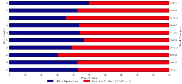
Galerkin Product

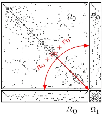
The construction of the sparse Galerkin product Ak+1 = RkAkPk in Line 6 of Algorithm 1 is typically implemented with two separate sparse matrix-matrix multiplies — i.e., (RA)P or R(AP) as shown in Figure 2.6. Either way, the first product is of the form [n×n]∗[n×nc] (or the transpose), while the second product is of the form [nc×n]∗[n×nc].

P

₀

Ω0

Ω1

R

₀

R

0

×

Ω 0

×

P

0

Figure 2.6: The unstructured nature ofP andAmakes generation of the coarse operator challenging.

Efficient sequential sparse matrix-matrix multiplication algorithms are described in [6, 40], where the Compressed Sparse Row (CSR) format is used, which provides O(1) indexing of the matrix rows. As a

(22)

result, the restriction matrixRk =PkT is formed explicitly in CSR format before the Galerkin product is computed. While the sequential algorithms for sparse matrix-matrix multiplication are efficient, they rely on a large amount of (per thread) temporary storage, and are therefore not suitable for fine-grained parallelism. Specifically, to compute the sparse productC=A∗B, the sequential methods useO(N) additional storage, whereN is the number of columns inC. In contrast, our approach to sparse matrix-matrix multiplication, detailed in Section 2.3.4, is formulated in terms of highly-scalable parallel primitives with no such limitations. Indeed, our formulation exploits parallelism at the level of individual matrix entries.

2.2.6

Spectral radius

For the smoothers such as weighted Jacobi or Chebyshev, a calculation of the spectral radius of a matrix — i.e., the eigenvalue of the matrix with maximum modulus — is often needed in order to yield effective smoothing properties. These smoothers are central to the relaxation scheme in the cycling phase and the prolongation in the setup phase, so we consider the computational impact of these calculations. Here, we use an approximation of the spectral radius ofD−1_A_where_D _{is matrix of the diagonal of}_A_.

To produce accurate estimates of the spectral radius we use an Arnoldi iteration which reduces A to an upper Hessenberg matrix H by similarity transformations. The eigenvalues of the small fixed-size dense matrix H are then computed directly. In Section 2.5, we see that computing the spectral radius has a non-trivial role in the total cost of the setup phase.

2.2.7

Cycling Phase

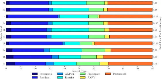
The multigrid cycling or solve phase is detailed in Algorithm 3 and illustrated in Figure 2.7. Several computations are executed at each level in the algorithm, but as we see in Lines 2-6, the operations are largely sparse matrix-vector multiplications (SpMV). Consequently, on a per-level basis, we observe a strong relationship between the performance of the SpMV and the computations in Lines 2-6. For example, the smoothing sweeps on Lines 2 and 6 are both implemented as affine operations such asxk←xk−ωD−1(Axk−

b), in the case of weighted Jacobi. This is a highly parallelized AXPY operation as well as a SpMV. This is

also the case for the residual on Line 3, and the restriction and interpolation operations on Lines 4 and 5. Finally, we coarsen to only a few points so that the coarse solve on Line 1 is efficiently handled by either relaxation or an arbitrary direct solver.

While the computations in the solve phase are straightforward at a high-level, they rely heavily on the ability to performunstructured SpMV operations efficiently. Indeed, even though the fine level matrix may exhibit a well-defined structure, the unstructured nature of the aggregation process produces coarse-level

(23)

Solve Presmooth

Restrict Prolongate

Postsmooth

Figure 2.7: Illustration of two-level V-cycle.

Algorithm 3: AMG Solve: solve parameters: Ak,Rk,Pk,xk,bk return: xk, solution vector if k=M

1 solveA_kx_k =b_k

else

2 xk ←presmooth(Ak, xk, bk, µ1) {smoothµ1 times onAkxk=_bk}

3 rk ←bk−Akxk {compute residual}

4 rk+1←Rkrr {restrict residual}

ek+1←solve(Ak+1, Rk+1, Pk+1, ek+1, rk+1) {coarse-grid solve}

5 e_k ←P_ke_k+1 {interpolate solution}

xk ←xk+ek {correct solution}

6 x_k ←postsmooth(A_k, x_k, b_k, µ₂) {smoothµ2 times onAkxk=bk}

matrices with less structure. In Section 2.5 we examine the cost of the solve phase in more detail.

2.2.8

Primitives

Our method for exposing fine-grained parallelism in AMG leverages data parallelprimitives[12, 75]. We use the term primitives to refer to a collection of fundamental algorithms that emerge in numerous contexts such as reduction, parallel prefix-sum (or scan), and sorting. In short, these primitives are to general-purpose computations what BLAS [54] is to computations in linear algebra. Like BLAS, the practice of distilling complex algorithms into parallel primitives has several advantages versus authoring ad hoc codes:

productivity: programming with primitives requires less developer effort,

performance: primitives can be optimized for the target architecture independently, portability: applications can be ported to a new architecture more easily.

Given the broad scope of their usage, special emphasis has been placed on the performance of primitives and very highly-optimized implementations are readily available for the GPU [58, 61, 75]. By basing our

(24)

AMG solver on these primitives we were able to implement the necessary components exclusively with the parallel primitives provided by the Thrust library [45]. This construction method is similar to the techniques typically utilized in the construction of dense linear algebra routines which base a complex set of architecture independent operations, such as those found in LAPACK, on a smaller set of reusable architecture dependent primitives, such as BLAS. Decoupling the algorithm from the implementation allows our implementation to achieve good performance while remaining flexible enough to execute on different architectures which expose the Thrust primitives.

2.3

Parallel Construction

In this section we describe an implementation of the multigrid setup phase (cf. Algorithm 1) using parallel primitives to expose the fine-grained parallelism required for GPU acceleration. Our primary contributions are parallel algorithms for aggregation and sparse matrix-matrix multiplication.

The methods described in this section are designed for thecoordinate (COO) sparse matrix format. The COO format is comprised of three arraysI,J, andV, which store the row indices, column indices, and values, respectively, of the matrix entries. We further assume that the COO entries are sorted by ascending row index. Although the COO representation is not generally the most efficient sparse matrix storage format, it is simple and easily manipulated.

2.3.1

Strength of Connection

The symmetric strength-of-connection algorithm (cf. Section 2.2.1) is straightforward to implement using parallel primitives. Given a matrixAin coordinate format we first extract the matrix diagonal by comparing the row index array,I, to the column index array,J,

D= [0,0,0,0],

is diagonal=transform(I,J,equals),

= [true,false,false,true,false,false,true,false,false,true],

D=scatter if(V,I,is diagonal,D), = [2,2,2,2],

and scattering the corresponding entries in the values array,V, when they are equal.

(25)

D[i]andD[j] for each index inIandJrespectively,

Di=gather(I,D),

= [2,2,2,2,2,2,2,2,2,2],

Dj=gather(J,D),

= [2,2,2,2,2,2,2,2,2,2],

from which the strength-of-connection threshold — i.e.,θp|D(In)| · |D(Jn)|in Algorithm 2 — of each entry is computed:

threshold=transform(Di,Dj,soc threshold(theta)),

using a specially-defined functor soc threshold. Next, each entry in the values array, V, is tested against the corresponding threshold to determine which entries are strong,

is strong=transform(V,threshold,greater),

= [true,true,true,true,true,true,true,true,true,true].

Finally, the matrix entries corresponding to strong connections are determined using stream compaction to form a coordinate representation of the strength-of-connection matrix, namely

Ci=copy if(I,is strong,identity),

Cj=copy if(J,is strong,identity),

Cv=copy if(V,is strong,identity).

In practice we do not construct arrays such as Di and threshold explicitly in memory. Instead, the gather and transform operations are fused with subsequent algorithms to conserve memory bandwidth using Thrust’s permutation iteratorandtransform iterator. Similarly, the three calls to copy ifare combined into a single stream compaction operation using azip iterator. The translation from the explicit version of the algorithm (shown here) and the more efficient, fused version (not shown) is only a mechanical transformation.

(26)

2.3.2

Aggregation

The sequential aggregation method (cf. Section 2.2.2) is designed to produce aggregates with a particular structure. Unfortunately, the greedy nature of the algorithm introduces sequential dependencies that prevent a direct parallelization of the algorithm’s first phase. In this section we describe a fine-grained parallel analog of the sequential method based on a generalizedmaximal independent set algorithm which produces aggregates with the same essential properties. A similar parallel aggregation strategy is described in [80], albeit with a different implementation.

There are two observations regarding the aggregation depicted in Figure 2.3 that lead to the description of our aggregation method. First, no two root nodes of the aggregates are within a distance of two edges apart. Second, if any unaggregated node is separated from all existing root nodes by more than two edges then it is free to become the root of a new aggregate. Together, these conditions define a collection of root nodes that are a distance−2 maximal independent set, which we denote MIS(2) and formalize in Definition 2.3.1. The first property ensures independence of the nodes — i.e., that the minimum distance between any pair of root nodes exceeds a given threshold. The second property ensures maximality — i.e., no additional node can be added to the set without violating the property of independence. The standard definition of a maximal independent set, which we denote MIS(1), is consistent with this definition except with a distance of one. We defer a complete description of the generalized maximal independent set algorithm to the Appendix. For the remainder of this section, we assume that a valid MIS(2) is computed efficiently in parallel.

Definition 2.3.1 (MIS(k)) Given a graphG= (V, E), let Vroot⊂V be a set of root nodes, and denote by

dG(·,·)the distance or shortest path between two vertices in the graph. Then,Vrootis a maximal independent set of distance k, or MIS(k) if the following hold:

1. (independence) Given any two verticesu, v∈Vroot, thendG(u, v)> k.

2. (maximality) There does not existu∈V \Vroot such thatdG(u, v)> kfor allv∈Vroot.

Given a valid MIS(2) the construction of aggregates is straightforward. Assume that the MIS(2) is specified by an array of values in{0,1}, where a value of 1 indicates that corresponding node is a member of the independent set and value of 0 indicates otherwise. We first enumerate the MIS(2) nodes with an exclusive scan operation, giving each set node a unique index in [0, N −1], where N is the number of nodes in the set. For example, on a linear graph with ten nodes, a MIS(2) with four set nodes,

(27)

is enumerated as

enum=exclusive scan(mis,0),

= [0,1,1,1,2,2,2,3,3,3].

Since thei-th node in the independent set serves as the root of thei-th aggregate, the only remaining task it so propagate the root indices outward.

The root indices are communicated to their neighbors with two operations resembling a sparse matrix-vector multiply, y = Ax. Conceptually, each unaggregated node looks at neighbors for the index of an aggregate. In the first step, all neighbors of a root node receive the root node’s aggregate index — i.e., the value resulting from theexclusive scanoperation. In the second step, the remaining unaggregated nodes receive the aggregate indices of their neighbors, at least one of which must belong to an aggregate. As before, in the presence of multiple neighboring aggregates a selection is made arbitrarily. The two sparse matrix-vector operations are analogous to the first and second phases of the sequential algorithm respectively — cf. Section 2.2.2. Our implementation of the parallel aggregate propagation step closely follows the existing techniques for sparse matrix-vector multiplication [10].

Figure 2.8 depicts a MIS(2) for a regular mesh and the corresponding aggregates rooted at each inde-pendent set node. Although the root nodes are selected by a randomized process (see the Appendix) the resulting aggregates are qualitatively similar to those chosen by the sequential algorithm in Figure 2.3a. Indeed, with the appropriate permutation of graph nodes, the sequential aggregation algorithm selects the same root nodes as the randomized MIS(2) method.

0 1 2 3 4 5 6 7 8 9 10 11 12 13 14 15 16 17 18 19 20 21 22 23 24 25 26 ₂₇ 28 29 30 31 32 33 34 35 36 37 38 39 40 41 42 43 44 45 46 0 1 2 3 4 5 6 7 8 9 10 11 12 13 14 15 16 17 18 19 20 21 22 23 24 25 26 ₂₇ 28 29 30 31 32 33 34 35 36 37 38 39 40 41 42 43 44 45 46 (a)MIS(2) 0 1 2 3 4 5 6 7 8 9 10 11 12 13 14 15 16 17 18 19 20 21 22 23 24 25 26 ₂₇ 28 29 30 31 32 33 34 35 36 37 38 39 40 41 42 43 44 45 46 0 1 2 3 4 5 6 7 8 9 10 11 12 13 14 15 16 17 18 19 20 21 22 23 24 25 26 ₂₇ 28 29 30 31 32 33 34 35 36 37 38 39 40 41 42 43 44 45 46 0 1 2 3 4 5 6 7 8 9 10 11 12 13 14 15 16 17 18 19 20 21 22 23 24 25 26 ₂₇ 28 29 30 31 32 33 34 35 36 37 38 39 40 41 42 43 44 45 46 (b)Aggregates

Figure 2.8: Parallel aggregation begins with a MIS(2)set of nodes, colored in gray, and represent the root of an aggregate — e.g., node 18. As in the sequential method, nodes adjacent to a root node are incorporated into the root node’s aggregate in the first phase. In the second phase, unaggregated nodes join an adjacent aggregate — e.g., nodes 12, 19, and 24 for root node 18.

(28)

2.3.3

Prolongation and Restriction

The tentative prolongation, prolongation smoothing, and restriction construction steps of Algorithm 1 (Lines 3, 4, and 5), are also expressed with parallel primitives. The tentative prolongation operation is constructed by gathering the appropriate entries from the near-nullspace vectors stored in B according to the sparsity pattern defined byN. Then, the columns are normalized, first by transposing the matrix, which has the effect of sorting the matrix entries by column index, and then computing the norm of each column using thereduce by keyalgorithm. Specifically, the transpose of a coordinate format matrix such as

I= 0 1 2 3 4 5 , J= 0 1 1 0 1 0 , V= 0 0 1 1 2 2 ,

is computed with by reordering the column indices of the matrix, and applying the same permutation to the rows and values

TransI,Permutation=stable sort by key(J,[0,1,2,3,4]) = 0 0 0 1 1 1 , 0 3 5 1 2 4 , TransJ=gather(Permutation,I) = 0 3 5 1 2 4 , TransV=gather(Permutation,V) = 0 1 2 0 1 2 .

Then the squares of the transposed values array are calculated, followed by row sums,

Squares=tranform(TransV,TransV,multiplies) =

0 1 4 0 1 4

,

Rows,Sums=reduce by key(TransI,Squares,multiplies) = 0 1 , 9 9 ,

(29)

which correspond to column sums of the original matrix.

Next, the final prolongator P is obtained by smoothing the columns of T according to the formula in Section 2.2.4. Here, we apply a specialized form of the general sparse matrix-matrix multiplication scheme described in Section 2.3.4. Specifically, we exploit the special structure of the tentative prolongator, whose rows contain at most one nonzero entry, when computing the expressionAT.

Finally, the transpose of the prolongation operator is calculated explicitlyR=PT_{, and Galerkin} triple-matrix product Ak+1 = Rk(AkPk) is computed with two separate sparse matrix-matrix multiplies. As mentioned above, the transpose operation is fast, particularly for the COO format.

2.3.4

Sparse Matrix-Matrix Multiplication

Efficiently computing the productC=AB of sparse matricesAandB is challenging, especially in parallel. The central difficulty is that, for irregular matrices, the structure of the output matrixC has a complex and unpredictable dependency on the input matricesA andB.

The sequential sparse matrix-matrix multiplication algorithm mentioned in Section 2.2.5 do not admit immediate, fine-grained parallelization. Specifically, for matrices A and B of size [k×m] and [m×n] the method requires O(n) temporary storage to determine the entries of each sparse row in the output. As a result, a straightforward parallelization of the sequential scheme requiresO(n) storage per thread, which is untenable when seeking to develop tens of thousands of independent threads of execution. While it is possible to construct variations of the sequential method with lower per-thread storage requirements, any method that operates on the granularity of matrix rows — i.e., distributing matrix rows over threads — requires a non-trivial amount of per-thread state and suffers load imbalances for certain input. As a result, we have designed an algorithm for sparse matrix-matrix multiplication based on sorting, segmented reduction, and other operations which are well-suited to fine-grained parallelism as discussed in Section 2.2.8.

As an example, we demonstrate our algorithm for computingC=AB, where

A=   5 10 0 15 0 20    and B =       25 0 30 0 35 40 45 0 50      , (2.6)

(30)

have 4 and 6 nonzero entries respectively. The matrices are stored in coordinate format as A=          (0,0, 5) (0,1,10) (1,0,15) (1,2,20)          and B =                 (0,0,25) (0,2,30) (1,1,35) (1,2,40) (2,0,45) (2,2,50)                 , (2.7)

where each (i, j, v) tuple of elements represents the row index, column index, and value of the matrix entry. We note that the (i, j, v) tuples are only a logical construction used to explain the algorithm. In practice the coordinate format is stored in a “structure of arrays” layout with three separate arrays.

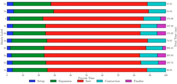
To expose fine-grained parallelism, our parallel sparse matrix-matrix multiplication algorithm proceeds in three stages:

1. Expansion ofABinto a intermediate coordinate formatT

2. Sorting ofT by row and column indices to form ˆT

3. Compression of ˆT by summing duplicate values for each matrix entry

In the first stage,T is formed by multiplying each entryA(i, j) of the left matrix with every entry in rowj

ofB,B(j, k) for all k. Here, the intermediate format is

T =                       (0,0, 125) (0,2, 150) (0,1, 350) (0,2, 400) (1,0, 375) (1,2, 450) (1,0, 900) (1,2,1000)                       , (2.8)

The expansion stage is implemented in parallel using gather, scatter, and prefix-sum operations. The result of the expansion phase is an intermediate coordinate format with possible duplicate entries that is sorted by row index, but not by column index. The second stage of the sparse matrix-matrix multiplication algorithm sorts the entries ofT into lexicographical order. For example, sorting the entries ofT by the (i, j)

(31)

coordinate yields ˆ T =                       (0,0, 125) (0,1, 350) (0,2, 150) (0,2, 400) (1,0, 375) (1,0, 900) (1,2, 450) (1,2,1000)                       , (2.9)

from which the duplicate entries are easily identified. The lexicographical reordering is efficiently imple-mented with two invocations of Thrust’sstable sort by keyalgorithm.

The final stage of the algorithm compresses duplicate coordinate entries while summing their corre-sponding values. Since ˆT is sorted by row and column, the duplicate entries are stored contiguously and are compressed with a single application of thereduce by keyalgorithm. In our example ˆT becomes

C=             (0,0, 125) (0,1, 350) (0,2, 550) (1,0,1275) (1,2,1450)             , (2.10)

where each of the duplicate entries have been combined. The compressed result is now a valid, duplicate-free coordinate representation of the matrix

AB=   125 350 550 1275 0 1450   .

All three stages of our sparse matrix-matrix multiplication algorithm expose ample fine-grained paral-lelism. Indeed, even modest problem sizes generate enough independent threads of execution to fully saturate the GPU. Furthermore, because we have completely flattened the computation into efficient data-parallel algorithms — i.e.,gather,scatter,scan,stable sort by key, etc. — our implementation is insensitive to the (inherent) irregularity of sparse matrix-matrix multiplication. As a result, even pathological inputs do not create substantial imbalances in the work distribution among threads.

(32)

com-plexity as the sequential method, which is O(nnz(T)), the number of entries in our intermediate format. Therefore our method is “work-efficient” [12], since (1) the complexity of the sequential method is propor-tional to the size of the intermediate format T and (2) the work involved at each stage of the algorithm is linear in the size of T. The latter claim is valid since Thrust employs work-efficient implementations of parallel primitives such asscan, reduce by keyandstable sort by key.

One practical limitation of the method as described above is that the memory required to store the intermediate format is potentially large. For instance, if A and B are both square, n×n matrices with exactly K entries per row, then O(nK2_{) bytes of memory are needed to store}_T_{. Since the input matrices} are generally large themselves (O(nK) bytes) it is not always possible to store aK-times larger intermediate result in memory. In the limit, ifA andB are dense matrices (stored in sparse format) thenO(n3_{) storage} is required. As a result, our implementation allocates a workspace of bounded size and decomposes the matrix-matrix multiplicationC =ABinto several smaller operations of the formC(slice,:) =A(slice,:)B, wheresliceis a subset of the rows ofA. The final result is obtained by simply concatenating the coordinate representations of all the partial results together C = [C(slice 0,:), C(slice 1,:), . . .]. In practice this sub-slicing technique introduces little overhead because the workspace is still large enough to fully utilize the device.

2.4

Parallel Multigrid Cycling

After the multigrid hierarchy has been constructed using the techniques in Section 2.3, the cycling of Algorithm 3 proceeds. In this section we describe the components of the multigrid cycling and how they are parallelized on the GPU.

2.4.1

Vector Operations

In Algorithm 3, the residual vector computation and the coarse grid correction steps require vector-vector subtraction and addition respectively. While these operations could be fused with the preceding sparse matrix-vector products for potential efficiency, or could be carried out withDAXPYin CUBLAS [26], we have implemented equivalent routines with Thrust’stransformalgorithm for simplicity. Similarly, the vector norms (DNRM2) and inner products (DDOT) that arise in multigrid cycling have been implemented with reduceandinner productin Thrust respectively.

(33)

2.4.2

Sparse Matrix-Vector Multiplication

Sparse matrix-vector multiplication (SpMV), which involves (potentially) irregular data structures and memory access patterns, is more challenging to implement than the aforementioned vector operations. Never-theless efficient techniques exist for matrices with a wide variety of sparsity patterns [7, 10, 13, 21, 30, 85, 86]. Our implementations of sparse matrix-vector multiplication are described in [10]. In Algorithm 3 sparse matrix-vector multiplication is used to compute the residual, to restrict the fine-level residual to the coarse grid, to interpolate the coarse-level solution onto the finer grid, and in many cases, to implement the pre-and post-smoother.

In Section 2.3 we describe a method for constructing the AMG hierarchy in parallel using the coordinate (COO) sparse matrix format. The COO format is simple to construct and manipulate, and therefore is well-suited for the computations that arise in the setup phase. However, the COO format is generally not the most efficient for the SpMV operations [10]. Fortunately, once the hierarchy is constructed it remains unchanged during the cycling phase. As a result, it is beneficial to convert the sparse matrices stored throughout the hierarchy to an alternative format that achieves higher SpMV performance.

Conversions between COO and other sparse matrix formats, such as CSR, DIA, ELL, and HYB [10], are inexpensive, as shown in Table 2.1. Here we see that the conversion from COO to CSR is trivial, while to more structured formats such as ELL and HYB is of minimal expense (note: the conversion to itself represents a straight copy). When reporting performance figures in Section 2.5 we include the COO to HYB conversion time in the setup phase.

From\To COO CSR ELL HYB

COO 5.09 6.35 20.10 23.55 CSR 7.80 4.03 21.61 24.84 ELL 17.02 18.26 5.90 22.32 HYB 63.27 69.40 83.08 4.12

Table 2.1: Sparse matrix conversion times (ms) for an unstructured mesh with 1M vertices and 8M

edges.

2.4.3

Smoothing

Gauss-Seidel relaxation is a popular multigrid smoother with several attractive properties. For instance, the method requires only O(1) temporary storage and converges for any symmetric, positive-definite ma-trix. Unfortunately, the standard Gauss-Seidel scheme does not admit an efficient parallel implementation.

(34)

Jacobi relaxation is a simple and highly parallel alternative to Gauss-Seidel, albeit without the same com-putational properties. Whereas Gauss-Seidel updates each unknown immediately, Jacobi’s method updates all unknowns in parallel, and therefore requires a temporary vector. Additionally, a weighting or damping parameterωmust be incorporated into Jacobi’s method to ensure convergence. The weighted Jacobi method is written in matrix form as, I− ω

ρ(D−1_A)D−1A, where D is a matrix containing the diagonal elements of

A. Since the expression is simply a vector operation and a sparse matrix-vector multiply, Jacobi’s method exposes substantial fine-grained parallelism.

We note that sparse matrix-vector multiplication is the main workhorse for several other highly-parallel smoothers. Indeed, so-called polynomial smoothers

x←x+P(A)r, (2.11)

whereP(A) is a polynomial in matrixA, are almost entirely implemented with sparse matrix-vector products. We refer to [1] for a comprehensive treatment of parallel smoothers and their associated trade-offs.

2.5

Experiments

In this section we examine the performance of a GPU implementation of the proposed method. We investigate both the setup phase of Algorithm 1 and the solve phase of Algorithm 3, and find tangible speed-ups in each.

2.5.1

Test Platforms

The specifications of our test system are listed in Table 2.2. Our system is configured with CUDA v4.0 [66] and Thrust v1.4 [45]. As discussed in Section 2.2.8, Thrust provides many highly optimized GPU parallel algorithms for reduction, sorting, etc. The entire setup phase, and most of the cycling phase, of our GPU method is implemented with Thrust. As a basis for comparison, we also consider the Intel Math Kernel

Testbed

GPU NVIDIA Tesla C2050

CPU Intel Core i7 950

CLOCK 3.07 GHz

OS Ubuntu 10.10

Host Compiler GCC 4.4.5 Device Compiler NVCC 4.0

Table 2.2: Specifications of the test platform.

(35)

subroutines such as sparse matrix-vector multiplication.

The Trilinos Project provides a smoothed aggregation-based AMG preconditioner for solving large, sparse linear systems in the ML package [34]. In our comparison, we use Trilinos version 10.6 and specifically ML version 5.0 for the solver. The ML results are presented in order to provide context for the performance of our solver in comparison to a well-known software package.

2.5.2

Distance-

k

Maximal Independent Sets

In this section we describe an efficient parallel algorithm for computing distance-k maximal independent sets, denoted MIS(k) and defined in Definition 2.3.1. We begin with a discussion of the standard distance-1 maximal independent set — i.e., MIS(distance-1) — and then detail the generalization to arbitrary distances. Our primary interest is in computing a MIS(2) to be used in the parallel aggregation scheme discussed in Section 2.3.2.

Computing a distance-1 maximal independent set is straightforward in a serial setting, as shown by Algorithm 4. The algorithm is greedy and iterates over nodes, labeling some as MIS nodes and their neighbors as non-MIS nodes. Specifically, all nodes are initially candidates for membership in the maximal independent set s and labeled (with value 0) as undecided. When a candidate node is encountered it is labeled (with value 1) as a member of the MIS, and all candidate neighbors of the MIS node are labeled (with value−1) as being removed from the MIS. Upon completion, the candidate set is empty and all nodes are labeled with either a−1 or 1.

Algorithm 4: MIS serial

parameters: A, n×nsparse matrix return: s, independent set

I={0, . . . , n−1} {initial candidate index set}

s←0 {initialize to undecided}

fori∈I {for each candidate}

if si= 0 {if unmarked. . .}

si = 1 {add to candidate set}

forj such thatAij 6= 0

sj =−1 {remove neighbors from candidate set}

s={i : si = 1} {return a list of MIS nodes}

Computing maximal independent sets in parallel is challenging, but several methods exist. With k= 1, our parallel version in Algorithm 5 can be considered a variant of Luby’s method [56] which has been employed in many codes such as ParMETIS [48]. A common characteristic of such schemes is the use of randomization to select independent set nodes in parallel.

(36)

Algorithm 5: MIS parallel

parameters: A,n×nsparse matrix;k, edge distance return: s, independent set

I={0, . . . , n−1}

s←0 {initialize state as undecided}

v←random {initialize value}

while {i∈I : si= 0} 6=∅

fori∈I {for each node in parallel}

Ti←(si, vi, i) {set tuple (state,value,index)}

1 forr= 1, . . . , k {propagate distancek}

fori∈I {for each node in parallel}

t←Ti

forj such thatAij 6= 0

t←max(t, Tj) {maximal tuple among neighbors}

ˆ

Ti←t

T = ˆT

2 fori∈I {for each node in parallel}

(smax, vmax, imax)←Ti

if si= 0 {if unmarked. . .}

if imax=i {if maximalldots}

si ←1 {add to set}

else if smax= 1 {otherwise. . .}

si ← −1 {remove from set}

(37)

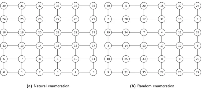
As with the serial method, all nodes are initially labeled (with a 0) as a candidate for membership in the MISs. Additionally, each node is assigned a random value in the arrayv. The purpose of the random value is to create disorder in the selection of nodes, allowing many nodes to be added to the independent set at once. Specifically, the random values represent the precedence in which nodes are considered for membership in the independent set. In the serial method this precedence is implicit in the graph ordering. Figure 2.9 illustrates a two-dimensional graph with random values values drawn from integers in [0, n= 36).

0 1 2 3 4 5 6 7 8 9 10 11 12 13 14 15 16 17 18 19 20 21 22 23 24 25 26 27 28 29 30 31 32 33 34 35

(a)Natural enumeration.

9 21 35 22 26 27 18 25 33 8 0 23 3 14 13 17 10 6 19 34 7 4 11 29 2 28 12 31 16 1 30 5 20 15 32 24 (b)Random enumeration.

Figure 2.9: A structured graph with a natural order of nodes and a randomized enumeration.

The algorithm iterates until all nodes have been labeled with a −1 or 1, classifying them as a non-MIS node or MIS node respectively. In each iteration, an arrayT of 3-tuples is created, tying together the node state — i.e.,−1, 0, or 1 — the node’s random value, and the linear index of the node. In a second phase, the nodes compute, in parallel, the maximum tuple among the neighbors. Given two tuples ti = (si, vi, i) and tj = (sj, vj, j) the maximum is determined by a lexicographical ordering of the tuples. This ordering ensures that MIS nodes have a priority over candidate nodes and that candidate nodes have priority over non-MIS nodes. In the third phase, the candidate node states are updated based on the results of the second phase. Candidate nodes that are the local maximum — i.e., Imax =i— are added to the independent set while those with an existing MIS neighbor — i.e.,Imax6=iand smax= 1 — are removed from candidacy. Since it is impossible for two neighboring nodes to be local maxima, the selected nodes are independent by construction. Furthermore, the correctness of the algorithm does not depend on the random values. Indeed, if all the random values are 0, the algorithm degenerates into the serial algorithm since the third component of the tuple, the node index, establishes precedence among neighbors with the same random value. In each iteration of the algorithm at least one candidate node’s state is changed, so termination is assured. Figure 2.10 illustrates the classification of nodes during six iterations of the parallel algorithm.

(38)

9 21 35 22 26 27 18 25 33 8 0 23 3 14 13 17 10 6 19 34 7 4 11 29 2 28 12 31 16 1 30 5 20 15 32 24 9 21 35 22 26 27 18 25 33 8 0 23 3 14 13 17 10 6 19 34 7 4 11 29 2 28 12 31 16 1 30 5 20 15 32 24 9 21 35 22 26 27 18 25 33 8 0 23 3 14 13 17 10 6 19 34 7 4 11 29 2 28 12 31 16 1 30 5 20 15 32 24 9 21 35 22 26 27 18 25 33 8 0 23 3 14 13 17 10 6 19 34 7 4 11 29 2 28 12 31 16 1 30 5 20 15 32 24 9 21 35 22 26 27 18 25 33 8 0 23 3 14 13 17 10 6 19 34 7 4 11 29 2 28 12 31 16 1 30 5 20 15 32 24 9 21 35 22 26 27 18 25 33 8 0 23 3 14 13 17 10 6 19 34 7 4 11 29 2 28 12 31 16 1 30 5 20 15 32 24 9 21 35 22 26 27 18 25 33 8 0 23 3 14 13 17 10 6 19 34 7 4 11 29 2 28 12 31 16 1 30 5 20 15 32 24 9 21 35 22 26 27 18 25 33 8 0 23 3 14 13 17 10 6 19 34 7 4 11 29 2 28 12 31 16