Subsurface exploration: engineering
geophysics
INTRODUCTION
The most widespread site investigation techniques, such as those described in Chapters 5, 7, 8 and 9, involve the drilling of holes in the ground, sampling at discrete points, and in situ or laboratory testing. Given the relatively small sums of money involved in ground
investigations of this type, only a very small proportion of the volume of soil and rock that will affect construction can be sampled and tested.
Geophysical techniques offer the chance to overcome some of the problems inherent in more conventional ground investigation techniques. Many methods exist with the potential of providing profiles and sections, so that (for example) the ground between boreholes can be checked to see whether ground conditions at the boreholes are representative of those elsewhere. Geophysical techniques also exist which can be of help in locating cavities, backfilled mineshafts, and dissolution features in carbonate rocks, and there are other techniques which can be extremely useful in determining the stiffness properties of the ground.
Yet, at the time of writing, geophysics is only rarely used in ground investigations. Various reasons have been put forward to explain this fact, including:
1. poor planning of geophysical surveys (see Chapter 1), by engineers ignorant of the techniques; and
2. overoptimism by geophysicists, leading to a poor reputation for the available techniques.
Most geophysics carried out during ground investigations is controlled by geologists or physicists. Generally, their educational background is either a geology or physics first degree, with a Masters postgraduate degree in geophysics. Such people often have considerable expertise in the geophysical techniques they offer, but they have very little idea of the contractual constraints within which civil and construction engineers must work. The writers’ view is that an understanding of geophysics is not beyond the capabilities of most civil engineers, who generally have a good education in physics. This chapter therefore provides an engineer’s view of engineering geophysics. It does not provide the conventional views of engineering geophysics, but deliberately concentrates on identifying those situations where geophysical techniques are likely to be of most help to engineers.
Engineering needs
Most geophysical techniques have as their origin the oil and mining industries. In such industries the primary need of a developer is to identify the locations of minerals for
exploitation, against a background of relatively large financial rewards once such deposits are found. Geophysics plays a vital role intermediate between geological interpretation of the ground and its structure, and the drilling of exploratory holes to confirm the presence of ores, oil or gas. In most cases the minerals are deep, and drilling is very expensive — geophysics
allows optimization of the drilling investigation, amongst other things. Many mineral explorations will be centred upon deep deposits, where ground conditions are spatially relatively uniform, and geological structures are large. Geophysical techniques are relatively cheap, and are highly regarded in such a speculative environment, even though they may not always be successful.
In contrast, ground investigations are carried out against a professional, contractual and legal background which often demands relatively fine resolution and certainty of result. The idea that a test or method will be successful and yield useful data only in a proportion of the cases in which it is used is unacceptable. As was noted in Chapter 1, it is necessary for a
geotechnical engineer to weigh carefully the need for each element of his ground
investigation. He will often have to persuade his client to provide additional funds for non-standard techniques, and if these are unsuccessful the client may not be convinced of his competence. Therefore, when using geophysical techniques during ground investigation, as part of the engineering design process, great care is needed. The engineer should convince himself of the need for such a survey, and should take care of ensure that only appropriate and properly designed surveys are carried out.
Unfortunately, there has been a widespread failure of geophysical techniques to perform as expected during ground investigations.
So far as geophysical methods of subsoil exploration are concerned, there can be no doubt about their desirability and merits, because they are extremely cheap: they are even cheaper than geologists. They have only one disadvantage, and that is we never know in advance whether they are going to work or not!
During my professional career, I have been intimately connected with seven geophysical surveys. In every case the physicists in charge of the exploration anticipated and promised satisfactory results. Yet only the first one was a success; the six others were rather dismal failures.
Terzaghi, 1957 More recently, the view has emerged that it is the planning of the surveys which has been at fault, and that if proper geological advice is sought then all will be well.
Too often in the past geophysical methods have been used without due reference to the geological situation, and consequently the results have been disappointing.
These failures always appear to be blamed on the method rather than on the misapplication of the method, and this is why many engineers mistrust geophysical methods. The solution to this difficulty is to take better geological advice during the planning of the investigation, and to maintain close
geological supervision during its execution.
Burton, 1975 It is our belief that both of these attitudes are over-simplistic. Whilst it is true that most professionals will be overoptimistic in their attempts to gain work, experience of the application of certain techniques during ground investigation is now sufficient to give guidance on techniques which will have a much better than one in seven chance of success. On the other hand, there is a growing trend for geophysical techniques to be integrated into ground investigations in a way which is difficult for a geophysicist to understand — the geophysicist cannot readily appreciate the engineer’s priorities and requirements, and may not be sufficiently familiar with the science of soil mechanics. In summary, the majority of problems arise because of:
2. poor inter-disciplinary understanding between engineers, engineering geologists and geophysicists;
3. a lack of communication, particularly with respect to the objectives of ground investigation;
4. a lack of objective appraisal of the previous success of geophysical techniques in the particular geological setting, given the objectives of the survey;
5. poor planning of the execution of the survey; and
6. the use of inappropriate science (for example, measurements of compressional wave velocities).
It is important to be clear as to the reason for using geophysics in ground investigations. In practice there are at least five different functions which can be fulfilled.
The variability of natural near-surface ground has already been noted, as has the limited finance available to make boreholes. Geophysical techniques can contribute very greatly to the process of ground investigation by allowing an assessment, in qualitative terms, of the lateral variability of the near-surface materials beneath a site. Non-contacting techniques such as ground conductivity, magnetometry, and gravity surveying are very useful, as are some surface techniques (for example, electrical resistivity traversing).
Geophysical techniques can also be used for vertical profiling. Here the objective is to determine the junctions between the different beds of soil or rock, in order either to correlate among boreholes or to infill between them. Techniques used for this purpose include electrical resistivity depth profiling, seismic methods, the surface wave technique, and geophysical borehole logging. Some are surface techniques, but the majority are carried out down-hole.
Sectioning is carried out to provide cross-sections of the ground, generally to give details of beds and layers. It is potentially useful when there are marked contrasts in the properties of the ground (as between the stiffness and strength of clay and rock), and the investigation is targeted at finding the position of a geometrically complex interface, or when there is a need to find hard inclusions or cavities. In addition, as with vertical profiling, these techniques can allow extrapolation of borehole data to areas of the site which have not been the subject of borehole investigation. Examples of such techniques are seismic tomography, ground probing radar, and seismic reflection.
One of the major needs of any ground investigation is the classification of the subsoil into groups with similar geotechnical characteristics. Geophysical techniques are not generally of great use in this respect, except in limited circumstances. An example occurs where there is a need to distinguish between cohesive and noncohesive soils. Provided that the salinity of the groundwater is low, it is normally possible to distinguish between these two groups of materials using either electrical resistivity or ground conductivity.
Finally, almost all geotechnical ground investigations aim to determine stiffness, strength, and other parameters in order to allow design calculations to be carried out. Traditionally,
geotechnical engineers felt that the determination of geotechnical parameters from
geophysical tests was impossible. The acceptance, within the last decade or so, that the small strain stiffnesses relevant to the design of civil engineering and building works may, in many circumstances be quite similar to the very small strain stiffness (Go or Gmax) that can be determined from seismic methods has led to a worldwide reawakening of interest in this type of method.
In selecting a particular geophysical technique for use on a given site, it is essential that the following questions are asked.
1. What is the objective of the survey?
It is generally true that users of geophysics expect the survey to provide a number of types of information. In fact, the converse is true. The survey should normally be designed to provide information on a single aspect of the site. A number of examples are given below:
• depth to rockhead;
• position of old mineshafts;
• corrosivity of the ground;
• very small strain stiffness of the ground;
• extent of saline intrusion of groundwater;
• position of cohesive and granular deposits along a pipeline route. 2. What is the physical property to be measured?
Given the ‘target’ of the geophysical investigation, the physical property that is to be measured may be obvious. For example, if the target is to be the determination of the very small strain stiffness of the ground, then it follows that the property that must be measured is the seismic shear wave velocity. But in many cases the success of a geophysical survey will depend upon the choice of the best geophysical method, and the best geophysical method is likely to be the one which is most sensitive to the variations in the ground properties associated with the target. For example, in trying to locate a mineshaft it might be relevant to consider whether metallic debris (for example, winding gear) has been left at the location (making magnetic methods likely to be successful) or whether the shaft is empty and relatively close to the ground (making gravity methods attractive).
3. Which method is most suited to the geometry of the target?
Geophysical targets range from cavities to boundaries between rock types, and from measurements of stiffness to the location of geological marker beds. The particular geometry of the target may make one particular technique very favourable (for example, the determination of the position of rockhead (i.e. the junction between rock and the overlying soil) or gassy sediments beneath the sea is often carried out using seismic reflection techniques.
4. Is there previous published experience of the use of this method for this purpose? Unfortunately it is unusual for engineers and geophysicists to publish their failures, so that the reporting of the successful use of a particular technique for a given target cannot be taken as a guarantee that it will work in a given situation. Conversely, however, the lack of evidence of success in the past should act as a warning. In assessing the likely success of a geophysical method, it will be helpful to consult as widely as possible with specialists and academic researchers.
Some geophysical methods have a very high rate of success, provided that the work is carried out by experienced personnel. Others will have very little chance of success, however well the work is executed.
5. Is the site ‘noisy’?
Geophysical methods require the acquisition of data in the field, and that data may be overwhelmed by the presence of interference. The interference will be specific to the chosen geophysical method; seismic surveys may be rendered impractical by the ground-borne noise from nearby roads, or from construction plant; resistivity and conductivity surveys may be interfered with by electrical cables, and gravity surveys will need to be corrected for the effects of nearby buildings, known basements, and embankments.
6. Are there any records of the ground conditions available?
If borehole or other records are available then two approaches are possible. The information can be used to refine the interpretation of the geophysical output, or the geophysical method can be tested blind. The latter method is really only suitable in instances where the geophysical method is claimed to work with great certainty, for example when testing a contractor’s ability to detect voids. In most cases
geophysicists will require a reasonable knowledge of the ground conditions in order to optimize the geophysical test method, and the withholding of available data will only jeopardize the success of a survey.
7. Is the sub-soil geometry sufficiently simple to allow interpretation?
Some methods of interpretation rely on there being a relatively simple sub-soil geometry, and one which is sufficiently similar to simple physical models used in forward modelling, to provide ‘master curves’. Most models will assume that there is no out-of-plane variability, and that the ground is layered, with each layer being isotropic and homogeneous. Complex three-dimensional structure cannot be interpreted.
8. Is the target too small or too deep to be detected?
9. Is it necessary to use more than one geophysical method for a given site?
Classification of geophysical techniques
There are many geophysical techniques available during ground investigation. In this section we attempt to classify them in different ways, to allow the reader to develop a framework within which to select the most appropriate technique(s) for his job.
Geophysical techniques may be categorized by the following: Control of input
Geophysical methods may be divided into two groups.
1. Passive techniques. The anomalies measured by the technique pre-exist. They cannot
be varied by the investigator. Repeat surveys can be carried out to investigate the effects of variations of background ‘noise’, but apart from varying the time of the survey, and the equipment used, no refinement is possible. In using passive
techniques, the choice of the precise technique and the equipment to be used are very important. Generally these techniques involve measurements of local variations in the Earth’s natural force fields (for example, gravity and magnetic fields).
2. Active techniques. These techniques measure perturbations created by an input, such
as seismic energy or nuclear radiation. Signal-to-noise ratio can be improved by adding together the results of several surveys (stacking), or by altering the input geometry.
In general, interpretation is more positive for active than for passive techniques, but the cost of active techniques tends to be greater than for passive techniques.
Types of measurement
Some geophysical techniques detect the spatial difference in the properties of the ground. Such differences (for example, the difference between the density of the ground and that of a water-filled cavity) lead to perturbations of the background level of a particular measurement
(in this case, gravitational pull) which are measured, and must then be interpreted. These perturbations are termed ‘anomalies’. Other geophysical techniques measure particular events (for example, seismic shear wave arrivals, as a function of time), and during interpretation these measurements are converted into properties (in this case, seismic shear wave velocity). A particular geophysical technique will make measurements of only a single type. Techniques that are commonly available measure:
• seismic wave amplitude, as a function of time;
• electrical resistivity or conductivity;
• electromagnetic radiation;
• radioactive radiation;
• magnetic flux density; and
• gravitational pull.
From a geotechnical point of view, passive techniques require relatively little explanation. The apparatus associated with them can often be regarded as ‘black boxes’. It is sufficient, for example, to note that:
1. gravity methods respond to differences in the mass of their surroundings, which results either from contrasts in the density of the ground, or from variations in geometry (cavities and voids, embankments, hills, etc.);
2. magnetic methods detect differences in the Earth’s magnetic field, which are produced locally by the degree of the magnetic susceptibility (the degree to which a body can be magnetized) of the surroundings. Such methods will primarily detect the differences in the iron content of the ground, whether natural or artificial;
3. Natural gamma logging detects the very small background radiation emitted by certain layers in the ground.
Active methods require more consideration, because surveys using these methods can often be optimized if the principles of the methods are understood.
The seismic method is rapidly becoming more popular in geotechnical investigations because
of its ability to give valuable information on the stiffness variations in the ground.
The seismic method relies on the differences in velocity of elastic or seismic waves through different geological or man-made materials. An elastic wave is generated in the ground by impactive force (a falling weight or hammer blow) or explosive charge. The resulting ground motion is detected at the surface by vibration detectors (geophones). Measurements of time intervals between the generation of the wave and its reception at the geophones enable the velocity of the elastic wave through different media in the ground to be determined. A seismic disturbance in elastically homogenous ground, whether natural or artificially induced, will cause the propagation of four types of elastic wave, which travel at different velocities. These waves are as follows.
1. Longitudinal waves (‘P’ waves). These are propagated as spherical fronts from the
source of the seismic disturbance. The motion of the ground is in the direction of propagation. These waves travel faster than any other type of wave generated by the seismic disturbance.
2. Transverse or shear waves (‘S’ waves). Transverse waves, like longitudinal waves,
are propagated as spherical fronts. The ground motion, however, is perpendicular to the direction of propagation in this case. S waves have two degrees of freedom unlike P waves which only have one. In practice, the S wave motion is resolved into
components parallel and perpendicular to the surface of the ground, which are known respectively as SH and SV waves. The maximum velocity of an S wave is about 70% of the P wave velocity through the same medium.
3. Rayleigh waves. These waves travel only along the ground surface. The particle
motion associated with these waves is elliptical (in the vertical plane). Rayleigh waves generally attenuate rapidly with distance. The velocity of these waves depends on wavelength and the thickness of the surface layer. In general, Rayleigh waves travel slower than P or S waves.
4. Love waves. These are surface waves which occur only when the surface layer has a
low P wave velocity with respect to the underlying layer. The wave motion is horizontal and transverse. The velocity of these waves may be equal to the S wave velocity of the surface layer or the underlying layer depending on the wavelength of the Love wave. Energy sources used in seismic work do not generate Love waves to a significant degree. Love waves are therefore generally considered unimportant in seismic investigation.
Soils generally comprise two phases (the soil skeleton and its interstitial water) and may have three phases (soil, water and air). P-wave energy travels through both the skeleton and the pore fluid, whilst S-wave energy travels only through the skeleton, because the pore fluid has no shear resistance.
Traditionally, the geophysical industry has made almost exclusive use of P waves. These are easy to detect, since they are the first arrivals on the seismic record. However, in relative soft saturated near-surface sediments, such as are typically encountered in the temperate regions of the world, the P-wave velocity is dominated by the bulk modulus of the pore fluid. If the ground is saturated, and the skeleton relatively compressible (i.e. B = 1 (Skempton 1954)), the P-wave velocity will not be much different from that of water (about 1500 m/s). Therefore it is not possible to distinguish between different types of ground on the basis of P-wave velocities until the bulk modulus of the skeleton of the soil or rock is substantially greater than that of water. This is only the case for relatively unweathered and unfractured rocks, for which the P-wave velocity may rise to as much as 7000 m/s.
Shear wave energy travels at a speed which is determined primarily by the shear modulus of the soil or rock skeleton, modified by its state of fracturing:
=
ρ
GVs (4.1)
where V, = shear wave velocity, G0 = shear modulus at very small strain and P = bulk density.
Since the bulk density of soil is not very variable, typically ranging from 1.6 Mg/rn3 for a soft soil to 3.0Mg/rn3 for a dense rock, the variation of S-wave velocity gives a good guide to the very small strain stiffness variations of the ground. Further, the last decade has brought a realization that (except at very small strain levels) soil does not behave in a linear-elastic manner, and that the strains around engineering works are typically very small. Thus it is now realized that stiffnesses obtained from geophysical methods may be acceptably close to those required for design. For rocks the operational stiffness may be very similar to that obtained from field geophysics, while for soils it is likely to be of the order of two or three times lower. Given the uncertainties of many methods available for determining ground stiffnesses, seismic geophysical methods of determining S-wave velocities are becoming increasingly important in geotechnical site investigations.
Whereas the determination of seismic shear wave velocity has gained increased prominence in site investigations, the use of seismic methods to determine the geometry of the sub-soil appears to have undergone a general decline. This is probably associated with a low level of success of these techniques in shallow investigations. The propagation of seismic waves through near-surface deposits is extremely complex. The particulate, layered and fractured nature of the ground means that waves undergo not only reflection and refraction but also diffraction, thus making modelling of seismic energy transmission impractical. Anisotropy, and complex and gradational soil boundaries often make interpretation impossible.
Electrical resistivity and conductivity methods rely on measuring subsurface variations of electrical current flow which are manifest by an increase or decrease in electrical potential between two electrodes. This is represented in terms of electrical resistivity which may be related to changes in rock or soil types. The electrical resistivity methods is commonly used therefore to map lateral and vertical changes in geological (or man-made) materials. The method may also used to:
1. assess the quality of rock/soil masses in engineering terms;
2. determine the depth to the water table (normally in arid or semi-arid areas); 3. map the saline/fresh water interface in coastal regions;
4. locate economic deposits of sand and gravel; and
5. locate buried features such as cavities, pipelines, clay-filled sink holes and buried channels.
The electrical resistivity of a material is defined as the resistance offered by a unit cube of that material to the flow of electrical current between two opposite faces. Most common rock-forming minerals are insulators, with the exception of metalliferous minerals which are usually good conductors. In general, therefore, rocks and soils conduct electricity by
electrolytic conduction within the water contained in their pores, fissures, or joints. It follows that the conductivity of rocks and soils is largely dependent upon the amount of water present, the conductivity of the water, and the manner in which the water is distributed within the material (i.e., the porosity, degree of saturation, degree of cementation, and fracture state). These factors are related by Archie’s empirical equation (Archie 1942):
l m wn s
aρ
ρ
= (4.2)where = resistivity of the rock or soil, w = resistivity of the pore water, n = porosity, s
degree of saturation, 1=2, m = 1.3-2.5, and a = 0.5-2.5.
The manner in which the water is distributed in the rock determines the factor m (cementation factor) which for loose (uncemented sands) is about 1.3 (Van Zijl 1978). The validity of Archie’s equation is, however, dependent on various factors such as the presence or absence of clay minerals (Griffiths 1946). Guyod (1964) gives a simplified version of Archie’s equation: 2
n
wρ
ρ
=
(4.3)where = resistivity of the rock/soil, w = resistivity of the pore water, and n = porosity.
Because the conduction of electrical current through the pore water is essentially electrolytic, the conductivity of the pore water must be related to the amount and type of electrolyte within it. Figure 4.1 shows the relation between the salinity of the pore water and the measured resistivity for materials with different porosities. As the salinity of the pore water increases,
The above relationships suggest that the more porous (or the more fissured/jointed) the soil or rock is, the lower is its resistivity. Thus, in general, crystalline rocks such as igneous rocks which exhibit a low porosity, have a high resistivity compared with the more porous sedimentary rocks such as sandstones. Clay-bearing rocks and soils will tend to have lower resistivities than non clay-bearing rocks and soils. These generalizations are reflected in the typical resistivity values for different soil and rock types given in Table 4.1.
Table 4.1 Typical electrical resistivity values for different soil and rock types
* Values from Dohr (1975).
† Values from Sowers and Sowers (1970). Degree of contact with the ground
The speed and cost of geophysical methods is strongly related to the amount of work necessary to set up the testing. Techniques (and therefore costs) vary very widely.
Non-contacting techniques are often relatively quick and easy to use. Examples are ground conductivity, magnetic and ground penetrating radar (GPR) techniques. Here the user carries the instrument across the site. Data are either collected automatically, on a time or distance basis, or upon demand (for example at predetermined positions, perhaps on a grid, across the site). These techniques are suitable for determining the variability of shallow soil or rock deposits, and can be economical ways of investigating large areas of ground in searches for particular hazards, such as mineshafts and dissolution features. Disturbance to the ground is minimal, and the equipment is often light enough to be carried by a single person.
Surface techniques are slower than non-contacting techniques, because sensor elements forming part of the geophysical measuring system must be attached to the ground before measurements can be made. Examples of such techniques are electrical resistivity, seismic refraction and reflection, and the surface wave technique. Although the method requires contact with the ground, it remains minimal and damage to the site will normally be negligible. Surface techniques are more expensive than non- contacting techniques, but can often allow a greater depth of investigation.
Down-hole techniques are generally the most expensive and time-consuming amongst the geophysical techniques. Sensors must be inserted down relatively deep preformed holes, or pushed to the required depth (perhaps 20m) using penetration testing equipment (see Chapter 5 and Chapter 9). Examples of this class of geophysics are seismic up-hole, down-hole and cross-hole testing, seismic tomography and down-hole logging. Despite their relative Material Resistivity ( m) Clay * 3-30
Saturated organic clay or silt † 5-20 Sandy clay * 5-40
Saturated inorganic clay or silt † 10-50 Clayey sand * 30-100 Hard, partially saturated clays † and silts, saturated sands and gravels † 50-150
Shales, dry clays, silts † 100-500 Sand, gravel * 100-4000 Sandstone * 100-8000 Sandstones, dry sands and gravels † 200-1000 Crystalline rocks * 200-10000 Sound crystalline rocks † 1000-10000 Rocksalt, anhydrite * >1100
slowness and cost, down-hole seismic techniques represent some of the best methods for use in geotechnical investigations, because they can be used to obtain good profiles of the very small strain stiffness of the ground.
Fig. 4.1 Effects of porosity and salinity of groundwater on measured resistivity (from Guyod, 1964).
Success rate
The success rate of geophysics depends greatly upon the care taken in its planning and execution. The planning of geophysics has been discussed in Chapter 1. Geophysical surveys should, in general, be carried out by experienced personnel.
In addition to the variable factors noted above, however, it should be recognized that some techniques are intrinsically more reliable, in a geotechnical setting, than others. This
perception of reliability stems from a combination of the way in which data are obtained and the purpose for which they are intended, and is tempered by a knowledge of the relative difficulty of obtaining data in other ways. Table 4.2 gives a brief summary of some of the most useful techniques for ground investigation.
Table 4.2 Geophysical methods with possible application in ground investigation
Application Possibly viable methods Comments
Lateral variability Ground conductivity Magnetometry Gravity
Electrical resistivity
These techniques are best used as an aid to selecting borehole locations. Preliminary borehole information will be particularly useful in selecting the best technique.
The depth investigated will generally be small (of the order of a few metres) so that these techniques will find most use on shallow, extended investigations, for example for pipelines.
Microgravity is claimed to have a high success rate in cavity detection. Vertical profiling Electrical resistivity depth probing
Natural gamma logging Seismic down-hole logging
Electrical resistivity depth probing is a surface technique which utilizes curve fitting for interpretation. Therefore the sub-soil geometry must be simple.
Geophysical logging of deep boreholes, for inter-borehole correlation, has been most
successfully carried out using natural gamma logs. It provides additional information at relatively little extra cost.
Sectioning Seismic tomography Ground penetrating radar Seismic reflection
Electrical resistivity imaging
Seismic tomography is a complex technique, which should be used with caution. It works best on deep sections. Its success rate in cavity detection is low. Ground penetrating radar is a shallow technique. Its technical development has been rapid in recent years, and it shows great promise for the future. Seismic reflection is best used over water, although development of shallow seismic reflection techniques may permit more land use in the future.
Ground classification Electrical resistivity
Ground conductivity Both techniques are limited to classifying the ground as cohesive or non-cohesive.
Stiffness determination Cross-hole seismic Up/Down-hole seismic Seismic tomography Surface wave
Seismic methods are generally successful, provided that background noise levels are low. They provide extremely valuable, and relatively cheap information on the stiffness of the ground.
LATERAL VARIABILITY
The positioning of boreholes on a site can only be carried out on the basis of geological maps and records, which generally give limited detail, or on grids or sections. Where large areas are to be investigated to shallow depth, the positioning of boreholes and trial pits becomes very difficult, since the aim is to sample representative ground. Similarly, when limited targets, such as dissolution features, mineshafts, and cavities are to be searched for, borehole investigation cannot be considered as viable. The cost of drilling holes precludes sufficient investigation to guarantee that all such hazards will be found. In these situations certain geophysical techniques can be very valuable, because they can cover large areas of ground at very little cost. The following techniques may prove useful.
Ground conductivity
Ground conductivity is an electromagnetic method. Electromagnetic methods are widely used in mineral exploration, in identifying materials that are relatively good electrical conductors and are at shallow depth. As the name implies, the method generally involves the propagation of continuous or transient electromagnetic fields in and over the ground. It can also use electromagnetic fields generated by others (i.e. the high-power VLF (very-low frequency) transmissions in the 15—25kHz range, which are used for air and marine navigation). Figure 4.2 shows the principle of operation of the Geonics EM31 and EM34 ground
conductivity meters, which are widely used in relatively shallow investigation work. They use Frequency Domain Electromagnetics (FDEM). The equipment comprises two vertical coplanar coils, each connected to a power source and a measuring instrument. There is no contact with the ground. The power source passes alternating current through coil A at a fixed frequency (of the order of 0.4—10kHz). The current in the coil produces a magnetic field whose magnitude varies continuously according to the strength of the current. This induces a current flow in the ground, which can be visualized as a third coil. The amount of current flow depends upon the conductivity of the ground, and controls the strength of magnetic field that it produces. This field changes continuously with time, and generates a current in coil B. Coil B also receives the direct magnetic field from the transmitter coil, coil A, and the instrument recording the current in coil B must be designed to distinguish between those currents directly induced by coil A, and those induced by the ground. Ground conductivity instruments of this type provide a direct readout (in millisiemens per metre) which is identical to that given by conventional resistivity instruments over a uniform half space. The output can be recorded continuously, and can be linked to a portable data acquisition unit, to allow rapid downloading of data to computer.
The EM31 (Fig. 4.3) is a lightweight (11kg) one-man instrument. It comprises a 4m long boom, with the coils mounted at both ends, with the operator controls and power pack at the centre. The effective depth of investigation is about 6m. The EM34 operates on the same principle, but uses two 63cm diameter coils which are carried by the two operators at a fixed spacing. The coils’ spacings may be l0m, 20m or 40m, and the instrument senses to about 0.75 of the intercoil spacing in the vertical coplanar mode. Both instruments give a rapid speed of survey, and produce data which are simple to use. The site is traversed with a given coil geometry, and the output data are simply located on plan, and contoured.
Fig. 4.3 Geonics EM31 ground conductivity meter
It has been noted that modern ground conductivity meters provide data which correspond to that produced by electrical resistivity meters. Therefore the main geotechnical use of ground conductivity will be the detection of contrasts in resistivity, which (as noted above) depends primarily on the clay content of the ground and the soluble salt content of the groundwater. Therefore, conductivity surveying can be a rapid method for differentiating between areas of cohesive and non-cohesive soil, and for detecting areas of groundwater contamination. The manufacturers claim that the EM31 can also be used to locate small metallic objects, such as small ore bodies or buried metal drums in waste sites.
Magnetometry
Magnetic methods are based on the measurement of local variations in the Earth’s magnetic field. Such variations are associated with differences in magnetic susceptibility (the degree to which a body is magnetized) of rocks and soils or the presence of permanently magnetized bodies. Since magnetic methods measure variations in a natural force field, the resulting data cannot be readily interpreted in a quantitative manner (i.e. depths and dimensions of
subsurface features cannot be determined directly from field data). Magnetic techniques are particularly useful in locating localized subsurface features of engineering interest such as abandoned mineshafts, sink holes, and buried services. The success rate in locating such features is moderate to good when used in favourable conditions. The main advantage however, of the method is the fact that magnetic measurements can be made extremely fast and hence the use of the method is reasonably cheap.
The measurements made in magnetic surveying may be of the vertical component of the Earth’s magnetic field or of the Earth’s total magnetic field strength. Measurements of the vertical component of the Earth’s magnetic field are made mechanically using magnetic balances. The total field strength is measured using fluxgate or proton instruments. For most engineering investigations the proton precession magnetometer is used. Extremely fast magnetic measurements can be made (usually less than 30s are spent at each station) using this instrument because it employs a remote sensing head which requires no levelling. The proton magnetometer is accurate to ± 1 nT1, compared with ±5 nT for the fluxgate instrument.
The strength of the Earth’s magnetic field varies between 47000 nT to about 49000 nT from south to north across the British Isles.
Observations are normally made on a grid. The station interval along each traverse line forming the grid should not exceed the expected dimensions of the feature to be located. A station interval of between 1 and 2m is normally used for the location of abandoned mineshafts. For the location of clay filled sink holes in chalk McDowell (1975) suggests a station interval (and distance between traverses) of less than half the expected lateral extent of the feature. The field data must be corrected for diurnal and secular variations in the Earth’s magnetic field. Diurnal variation is measured throughout the survey by periodically returning to a base station and measuring the field strength. The field data once corrected for these variations are normally presented in the form of a contoured magnetic map. Figure 4.4 shows a magnetic map for a site at Mangotsfield, Bristol. The contour values are relative to the regional magnetic field strength. Characteristic shapes may be recognized from magnetic maps and related to subsurface bodies in terms of general geometry and orientation (if they are not equidimensional) magnetic profiles are often drawn across anomalies to aid interpretation.
Interpretation of magnetic data is qualitative. Detailed analysis of the data may be carried out by comparing field data with theoretical anomalies produced by physical models. These models are altered to produce a best fit with the field data. The field data, however, can be highly ambiguous and a unique relationship between the anomalies produced by a single physical model and the field prototype rarely exists. In some cases the depth of a subsurface feature may be estimated from the width of the anomaly produced.
Measured field strengths are seriously affected by interference from electrical cables, electric railways, moving vehicles and highly heterogeneous ground. The latter is a common feature of urban areas in which the abundance of old foundations, buried services, and waste material gives rise to complex anomalies which can easily mask anomalies produced by singular features of engineering interest.
Ideal sites for the use of magnetic methods are on open little-developed land, free from extraneous interference. The method may be used successfully in developed areas, but care should be taken in choosing the magnetic method. Moreover, the engineering geophysicist should be presented with all the available data concerning the history of the site, which may have been obtained during the preliminary desk study.
The magnitude of magnetic anomalies associated with localized features will depend on the depth of the feature and the height of the sensor above the ground. A sensor height of 1 m above ground level has proved convenient and adequately free from magnetic variations of the top soil (Hooper and McDowell 1977). In general, the magnetic anomaly produced by a subsurface feature decreases rapidly as the depth of overburden increases. This can make detection of deep features difficult, particularly if they are of limited extent and do not show a very high susceptibility contrast with the surrounding ground. Anomalies produced by local features generally become difficult to identify when the lateral dimensions are less than the
depth of the cover. The maximum depth of burial at which the detection of abandoned mineshafts generally becomes difficult is about 2—3m depending on the diameter of the shaft and the magnetic susceptibility contrast with the surrounding material. The magnitude and shape of the anomaly produced by elongate (or linear) features (i.e. elongate in the vertical plane) .such as dykes are affected by the orientation of the feature as well as the orientation of the magnetic field. Linear features which trend magnetic north— south are difficult to locate.
Fig. 4.4 Magnetic field strength map of Mangotsfield, Bristol (after Hooper and McDowell, 1977).
The advantage of magnetic methods is the speed at which measurements can be taken. With a proton magnetometer it is possible to cover an area of 1500 m2 in a day taking measurements on a 1 m grid. It is possible to cover 1000 m2 in 60 mm taking measurements on a 2 m grid with the less sensitive fluxgate magnetometer (Dearman et a!. 1977). Since essentially only one correction is applied to the field measurements, data reduction, presentation and interpretation can be carried out rapidly. Clearly the magnetic methods can be most cost effective in site investigations that require localized features at shallow depths to be located provided of course that the conditions are recognized as being suitable for the method to have a reasonable chance of success.
The main use of magnetic methods in site investigation appears to be for the location of abandoned mineshafts. The successful location of such features using magnetic methods has been reported by Raybould and Price (1966), Maxwell (1976), Dearman et al. (1977) and Hooper and McDowell (1977). It is unfortunate, however, that unsuccessful cases are not also reported, as these are equally (if not more) numerous than the successful cases. The
publication of unsuccessful cases would give a better insight to some of the drawbacks of the method and perhaps allow some improvements to be made. The main problem in detecting abandoned shafts is that there is a great variety of anomalies associated with these features. Each shaft may be different from another in terms of:
1. whether it is capped or uncapped: 2. the type of capping material; 3. the type of shaft lining;
4. the type of shaft infilling material (if present); 5. groundwater table; and
6. the nature of the surrounding debris.
Thus all anomalies must be investigated by direct methods. Often the method is used in the wrong conditions, such as areas where the ground is particularly heterogeneous (which is not unusual in mining areas) or areas where there is likelihood of extraneous interference. The chances of success in such cases are minimal. The limitations of the method mentioned earlier clearly reduce the number of situations where success is possible.
When using the magnetic methods to locate geological features it should be borne in mind that the method was initially developed for prospecting and was used to locate large-scale geological features. If the geology beneath a site is particularly complex, interpretation of magnetic data will be difficult, if not impossible, in extreme cases. Locally complex geology will also present problems in locating man-made features.
McDowell (1975) discusses the use of magnetic methods in the detection of clay- filled sink holes in chalk. In favourable circumstances the proton precession magnetometer can be used to locate these features very rapidly and at little cost compared with employing direct methods of investigation, or other geophysical methods. A magnetic map for a test site in Upper Enham, Hampshire, is shown in Fig. 4.5.
The magnetic method may also be used to locate basic igneous dykes below a cover of superficial deposits (Higginbottom 1976) and buried services such as clay or metal pipes.
Electrical resistivity traversing
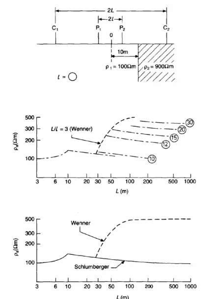
Resistivity traversing is normally carried out to map horizontal changes in resistivity across a site. Lateral changes in resistivity are detected by using a fixed electrode separation and moving the whole electrode array between each resistivity. The interpretation of resistivity traverses is generally qualitative unless it is carried out in conjunction with sounding techniques. The use of traversing and sounding together is quite common in resistivity surveying (for example, see McDowell (1971)). The electrode configurations normally used in electrical traversing are the Wenner configuration and the Schlumberger configuration, Table 4.3. The Wenner configuration has the simplest geometry and is therefore easier to use and quicker than employing a Schlumberger configuration. If the resistivity station interval is the same as the electrode spacing it is possible to move from station to station along a traverse line by moving only one electrode each time. This is not possible with a Schlumberger configuration as the potential electrode spacing is not one-third of the current electrode spacing.
Resistivity equipment passes a small low-frequency a.c. current (of up to 100 mA) to the ground via the current electrodes (C1 and C2). The resistance between the potential electrodes (P1 and P2) is determined by measuring the voltage between them. This voltage is normally amplified by the measuring device. The current source is then switched to an internal bridge circuit (via the amplifier) in which a resistance is altered using a potentiometer to give the same output voltage as measured between the potential electrodes. In general, as the electrode spacing is increased the measured resistance decreases. It is therefore necessary for the equipment to be capable of measuring small resistances. The resistances that may be measured with some a.c. devices are in the range 0.0003 to 10 k (ABEM Terrameter).
measured resistance. The way in which it is determined will depend upon the electrode configuration used. Over homogeneous ground the measured resistivity will be constant for any electrode configuration. The ground is, however, rarely homogeneous and, in practice, the measured resistivity will depend upon the electrode configuration. This measured resistivity for any electrode configuration is called the apparent resistivity.
Fig. 4.5 Magnetic field strength map of Upper Enham, Hampshire (after McDowell 1975). Modern resistivity meters are compact and portable. Portability of equipment is an important factor which affects the logistics of the survey, particularly when traversing.
The location of localized subsurface features such as abandoned mineshafts and cavities often requires the use of less common electrode configurations, in order to increase the sensitivity to lateral changes in resistivity which are of limited lateral extent. The central electrode configuration shown in Table 4.3 generally gives a smoother profile and larger amplitude anomalies over small features than the conventional Wenner or Schlumberger arrays. With the central electrode configuration only the potential electrodes are moved between each measurement, and hence traversing can be carried out rapidly. A 30 m long traverse with a 1 m station interval can be completed in about 30mm. with a two-man team, whereas 60mm. is required when using a Wenner configuration (with a = 2 m). The disadvantage of this electrode configuration is that the distance factor changes for each station making it difficult for the observer to form a picture of the pattern of anomalies directly from the field data. Spurious measurements are therefore too easily missed until the apparent resistivities are calculated.
The Wenner configuration has the disadvantage of producing large flanking anomalies adjacent to anomalies produced by sharp changes in resistivity (Fig. 4.6). This can be a serious limitation, particularly when using the method to locate localized subsurface features, such as sink holes, buried channels or abandoned mineshafts, as the flanking anomalies can mask the main anomaly (Cook and Van Nostrand 1954). The Schlumberger configuration will
in the same situation cause the main anomaly to be enhanced and the flanking anomalies to be reduced.
Table 4.3 Types of electrode configuration commonly used in resistivity surveying Type of electrode
configuration
Sketch of electrode
configuration Distance factor Comments
Wenner 2 πa Not suitable for location of
narrow steep-sided features, such as fault zones and dissolution features because of flanking anomalies. All four electrodes are moved when traversing. Schlumberger l l L 2 ) ( 2− 2
π Reduces flanking anomalies.
Sensitivity with increased depth, drops less rapidly than with Wenner. All four electrodes are moved when traversing. Central electrode ) ) ( 1 ) ( 1 ( 2 b c c b a a b + + +
π Suitable for location of sharp changes in resistivity. Traversing is rapid as current electrodes are not moved. Pole-dipole ) ( 2 a b ab −
π Remote current electrode
C2. It is not necessary to have C2 in line with the other electrodes. Configuration permits lateral exploration on radial lines from a fixed position of C2. Suitable for resistivity mapping in the vicinity of a conductor of limited extent.
Double-dipole
(dipole-dipole) 2πnl(n−1)(n+1) Common configuration used with induced polarization work. n must be less than or equal to 5.
The electrical resistivity method has been used with limited success in the detection of cavities. In view of the time required for a resistivity survey compared with that required for a magnetic survey (discussed above), the resistivity method is not as cost effective in view of the small chances of success. A successful attempt to locate abandoned mineshafts using electrical resistivity is reported by Barker and Worthington (1972).
Resistivity techniques have been used successfully in arid and semi-arid areas in groundwater investigations. Some case histories are given by Martinelli (1978). Krynine and Judd (1957) report the use of the electrical resistivity method to locate and assess the nature of faults and fracture zones suspected of running parallel to a proposed tunnel line. Resistivity methods have also been used to locate and map the extent of fissures in karst dolomite for the foundation design of a dolomite processing plant near the town of Matlock (Early and Dyer 1964).
Fig. 4.6 Theoretical flanking anomalies produced over the edges of localised features (after Cook and Van Nostrand 1954).
Gravity methods
Gravity methods involve measuring lateral changes in the Earth’s gravitational field. Such variations are associated with near-surface changes in density and hence may be related to changes in soil or rock type. Because gravity methods involve the measurement of a natural force field, ambiguous data (in terms of interpretation) are common and hence the
interpretation of field data is qualitative. The effects of rapid near-surface changes in density limit the use of this method in practice to the mapping of large- scale geological) structures. This can be of great value in oil exploration but on the very much smaller scale of engineering site investigations it seriously restricts the use of gravity measuring techniques. Gravity methods may be used for the location of large faults and to find the extent of large buried channels.
As mentioned earlier, density does not vary greatly between different soils and rocks. Thus local variations in gravity (gravity anomalies) will be small compared with the overall gravitational field strength. Gravity measuring instruments must therefore be extremely sensitive. Gravity meters comprise sensitive balances such that small variations are magnified by mechanical or mechanical and optical methods to enable readability. Only the vertical component of gravity is measured with these instruments.
The acceleration of gravity is measured in units of milligals (1 milligal =10 -5 m/s2). Gravity
meters have a sensitivity of about 1 part in 108 of the Earth’s gravitational field which represents a resolution 0.01 milligal. The most sensitive gravity meter has a resolving power in the microgal range.
Measured values of the vertical component of the gravitational field are not only a function of density but also a function of latitude, elevation, local topography, and tidal effects. The effects of these on gravity measurements can be determined and corrections made. Every field measurement must be reduced by applying the following corrections.
1. Latitude correction. This is applied because the Earth is not a perfect sphere and hence the gravitational force varies between the poles and the equator.
2. Elevation correction. This is applied to reduce all gravity measurements to a common
elevation. The correction is in two parts.
(i) Free air correction. This is made for the displacement of the point of
observation above the reference level (usually ordnance datum O.D.). This requires the levelling of the gravity meter to within 0.05 m.
(ii) Bouguer correction. This is applied to remove the effect of the material
between the gravity meter and the datum level. This requires the density of the material to be known (usually it is estimated).
3. Terrain correction. This is applied to remove the effects of the surrounding
topography. The correction is obtained from a graphical determination of the gravity effect at the observation point of all hills and valleys. The correction is usually calculated to about 20km out from the station but where relief is low the survey area considered for this correction is reduced (Higginbottom 1976).
4. Instrument drift and tidal correction. These corrections are made by returning to a base station and measuring the field strength at frequent intervals during the survey. The corrected gravity measurements are known collectively as Bouguer anomalies.
A gravity survey requires an accurate topographic survey of the site and surrounding area to be carried out to enable some of the corrections to be applied to the field data. In the British Isles most of the topographic data necessary may be obtained from Ordnance Survey maps and plans. Each observation point must however be accurately levelled. Clearly the
acquisition and reduction of gravity data are extremely time- consuming and hence expensive. The corrected gravity data are normally presented as a contoured gravity map (Isogal map). The contour values may represent Bouguer anomalies or residual gravity values. Residual gravity values are derived from the difference between the regional Bouguer anomaly and the local Bouguer anomaly.
These gravity maps allow anomalies to be readily identified (if of sufficient magnitude) and thus target areas are defined for direct investigation. Figure 4.7 shows examples of the different forms of gravity maps.
To enable detection of subsurface features the amplitude of the gravity anomaly produced must be at least 0.2 mgal. Most features of engineering interest produce anomalies which are much smaller than this and in most cases may be detected more efficiently by other
geophysical methods. The main exception according to Higginbottom (1976) is the case of faults with displacements large enough to introduce materials of different density across the fault plane, but where the contrast between other physical properties is slight. A density contrast may also give rise to a P-wave velocity contrast. It would be easier therefore to use a seismic method such as seismic refraction if this were the case.
The gravity method has been used to aid determination of the cross-section of an alluvium filled valley in North Wales (Fig. 4.7, see Griffiths and King (1965), for discussion) and the location of cavities (Colley 1963).
In general, gravity methods are too slow and expensive to be cost effective in conventional site investigations. Only in rare circumstances are the use of gravity methods justified particularly as justification must normally be based on the limited information available at an early stage of the investigation.
In contrast with conventional gravity surveys, which are generally concerned with large-scale geological structures and the identification of different rock types over large areas of ground,
micro-gravity surveys are limited both in extent and objectives. Station spacings may be as close as 1 m, and the normal use of micro-gravity is in the construction industry, to detect subsurface cavities. Here the target has a large density contrast with that of the surrounding ground so that, provided it is sufficiently shallow and there is little ‘interference’ in the form of complex geometry (for example from the gravitational pull of surrounding buildings, or the effects of nearby embankments, tunnels or basements), the method should be of use in what is otherwise a particularly difficult problem area for geotechnical engineers.
Fig. 4.7 Different types of gravity map for the Harlech, Portmadoc area of North Wales (from Griffiths and King 1965).
Typically, microgravity surveys may involve between 100 and 400 gravity stations with spacings as close as 1 m. The stations are levelled (using precise levelling equipment) and gravity measurements made to a resolution of 1 gal. Typical anomalies associated with shallow (0—l0m) features (e.g. voids, dissolution features and disturbed ground) are between 20 and 100 gal. Using a portable PC, preliminary data processing may be carried out on site in order to confirm adequate definition of anomalies.
PROFILING
Most ground investigations will not make use of geophysical methods for profiling. This will normally be done by describing the material arising from boreholes, or by carrying out probing tests (Chapter 5). Exceptions may occur when there is need for information from areas between boreholes, or where boreholes are deep, and there is a need to correlate between them. Profiling can be carried out by identifying the characteristics of the material within each bed, or by identifying marker beds which are common to all boreholes.
Whilst electrical resistivity can be used for this purpose, it is not common. Seismic probing is on the increase, and natural-gamma logging has long been used for inter- borehole
correlations when deep investigations are being carried out.
Electrical resistivity sounding
Vertical changes in electrical resistivity are measured by progressively moving the electrodes outwards with respect to a fixed central point. The depth of current penetration is thus increased. Any variations in electrical resistivity with depth will be reflected in variations in measured potential difference.
Electrical sounding involves investigating a progressively increasing volume of ground. As the vertical extent of this volume increases so will the lateral extent. Lateral variations in electrical resistivity will therefore introduce errors when determining variations of resistivity with depth. Ideally the lateral dimensions of the volume of ground under consideration should be kept relatively small compared with the vertical dimension. Electrical sounding using the Wenner configuration (Table 4.3) requires that both the current and potential electrode separations are increased between each resistivity measurement. The lateral dimensions are therefore allowed to become large. Thus Wenner sounding is likely to produce an erroneous resistivity/depth relationship because of lateral variations in resistivity.
When electrical sounding with a Schlumberger configuration is used the potential electrode spacing is kept small (potential electrode spacing 0.2 current electrode spacing) and only the current electrode spacing is increased between each resistivity measurement. The potential electrode spacing is only increased when A V becomes very small and in this way the minimum lateral dimension condition is more-or-less satisfied. Thus the results of
Schlumberger sounding are less prone to error due to lateral changes in resistivity. Figure 4.8 shows the effect of a lateral change in resistivity on the results of electrical sounding using Wenner and Schlumberger configurations.
When using the Wenner array the errors due to lateral changes in resistivity may be greatly reduced and often eliminated by the use of the Offset Wenner system. The principles of this system may be summarized by considering the ‘signal contributions section’ for a Wenner array shown in Fig. 4.9. For homogeneous ground the positive and negative contributions of high magnitude cancel each other out and the resultant signal originates mainly from depth and not from the region around the electrodes. If, however, a high resistivity body (for example, a boulder) is located in the positive zone, the measured resistance will be greater
contributing zone the measured resistance will be lower. In each case the body will cause an error in the resistance measurement. The effect of the body may be reduced by measuring the resistance with the body in the negative zone and then moving the electrode array such that the body is in a positive zone and taking a second resistance measurement. If the two resistance measurements are averaged, the effect of the body is eliminated or at least greatly reduced.
Fig. 4.8 Comparison of data produced by different electrode configurations across a sharp lateral change in resistivity (after Van Zijl 1978).
In practice, Offset Wenner sounding is conducted using a five-electrode array as shown in Fig. 4.10. When using this array the additional electrode remains fixed at the centre of the spread and a switching device is used to change from one adjacent set of four electrodes to the other. Two resistances (RD1 and RD2) are measured and averaged to obtain the Offset Wenner
resistance RD. If the spacing is increased according to the series a=0.5, 1, 2, 4, 8, 16, 32, 64... 2n m, so that the potential electrode always falls on a position previously occupied by a
current electrode, the necessary data required for depth sounding may be obtained. In practice, sounding data are acquired by placing electrodes at all the electrode positions to be used and attaching them to two multicore cables as shown in Fig. 4.11. The connection points on the multicore cable may be positioned at the necessary spacings to reduce the time spent in
setting out the array. Two resistance readings are taken for each electrode spacing using a switching device and a digital resistivity meter. A portable computer may be used to control the switching device and to store the resistivity measurements. The advantages of the Offset Wenner sounding system include the following.
1. Near-surface lateral resistivity variations are greatly reduced and this results in a sounding curve which is smoother than both the comparative Wenner and Schlumberger curves.
2. The whole system may be carried and operated by one person. Using modern lightweight equipment a sounding may be conducted in much less than one hour. 3. A conventional Wenner apparent resistivity curve is obtained.
4. The magnitude of lateral resistivity effects may be estimated. This estimate is provided by the ‘Offset error’ defined by the following expression:
% 100 _ = 1− 2 × D D D R R R error Offset
Fig. 4.9 Signal contribution for a Wenner array.
Fig. 4.10 Principles of sounding with Offset Wenner five-electrode array.
If the offset error is systematically greater than 10% the interpretation of the apparent resistivity curve may be significantly in error. Although the Offset technique substantially
dipping strata and faults are likely to distort the sounding curve seriously. The Offset error will indicate when such situations are encountered.
Fig. 4.11 Arrangement for Wenner Offset sounding using multicore cable and switch box for a=0.5, 1,2,4,8, 16, 32 and 64m.
The major potential disadvantage of Offset Wenner and conventional Wenner sounding is the large electrode spacing required to obtain a significant depth of current penetration. For example a typical Offset Wenner spread with amax = 64 m has a total length of 256 m. This is
clearly a limitation when using these methods on restricted sites. The Schlumberger
configuration requires a smaller current electrode spacing to achieve similar depths of current penetration.
Errors in apparent resistivity measurements can be caused by the following.
1. Electromagnetic coupling between potential and current electrode cables. This may
be overcome by ensuring that current and potential electrode cables do not cross each other, are not laid very close to each other or are adequately shielded.
2. Interference from high (or low) tension electrical cables or electrified railway lines. Sounding or profiling near electrical cables of any sort should be avoided. The interference from overhead high tension cables can be reduced by having the azimuth of the electrode array parallel to the line of the cables.
3. Highly heterogeneous ground. If the surface layer is highly heterogeneous due to
complex geology, buried services, old foundations, root holes, or waste material, errors may be introduced in sounding data even when a Schlumberger configuration is used.
Quantitative interpretation of electrical sounding data is possible using various curve matching techniques. The measured values of apparent resistivity are plotted as a function of current electrode spacing. For Wenner configurations a is plotted as a function of a (1/3
current electrode spacing) and for Schlumberger configurations a is plotted as a function of L
(1/2 current electrode spacing). Logarithmic scales are normally employed as this facilitates direct curve matching techniques since there are no problems in comparison of data due to the
use of different scales. The pattern of current distribution through a stratified media can be derived theoretically. Thus theoretical curves (master curves) of apparent resistivity against electrode spacing can be produced (on logarithmic scales). Such curves have been computed for strata parallel to the ground surface by Mooney and Wetzel (1956) and Mooney and Orellana (1966). A full set of master curves for strata parallel to the ground surface is published by La Compagnie Générale de Géophysique (1963). An example of one set of master curves is given in Fig. 4.12. These master curves are matched with the field curves. The master curve which best matches the field curve can be used to determine the apparent resistivities and the depths of each layer detected in the field. Figure 4.13 shows some field data on which a best-fit master curve has been superimposed. The field curve will never exactly match the master curve because of undulating or dipping interfaces which cannot be represented in a finite set of master curves. Thus a subjective element is introduced in the curve matching process and the choice of physical model must be aided by a knowledge of the likely geological succession and groundwater conditions. Preliminary electrical soundings are therefore carried out where possible close to the site of a borehole or near an exposure to provide a control over interpreting subsequent electrical soundings. Data processing
techniques now allow a more objective approach to be made in finding a physical model which best represents the field prototype. Most sets of published master curves are for strata which are parallel to the ground surface and it is therefore necessary to have prior knowledge of the local dip and strike of the strata beneath the site. It is most unlikely that the ground surface will have the same inclination (in both magnitude and direction) as the dip of the strata beneath it and it is therefore necessary to attempt to orientate the azimuth of the
electrode array along the strike of the dipping strata. This is not always possible as the ground may not be horizontal in this direction. Clearly this is a serious limitation of the electrical sounding method. Master curves for dipping strata have been computed by Maeda (1955), but the number of curves involved tends to over-complicate interpretation by curve matching alone. The dipping strata problem tends to lend itself to the more modern data processing techniques.
Fig. 4.12 Typical set of master curves for Schlumberger sounding (Compagnie Générale de Géophysique 1963).
The computation of master curves is based on the assumption that each layer considered is isotropic and homogeneous in terms of resistivity. This is rarely true in soils and rocks and can lead to ambiguities in interpretation and hence serious errors in depth determinations. In
made between isotropic and anisotropic layers. The degree of resistivity anisotropy in anisotropic layers is generally greater than unity and hence depths are overestimated.
Anisotropy of the clay overlying the chalk in Fig. 4.13 is likely to be the reason why the depth of the top of the chalk is overestimated by the interpretation of the resistivity data.
Fig. 4.13 Interpretation of electrical resistivity sounding data.
Seismic profiling
A relatively quick method of obtaining a profile which will approximate to ground stiffness is to drive a probe or penetrometer into the ground, using it either as a seismic source, or as a receiver if geophones are incorporated into it.
The seismic cone is one of a large family of cone penetrometers (see Chapter 5) which are widely used in geotechnical investigation, particularly in relatively soft ground. Essentially the device consists of a solid metal shaft, 10cm2 in cross-sectional area and with a 60° cone end, which is pushed hydraulically into the ground. By mounting geophones in the cone, the arrival of seismic waves can be detected, and these can be interpreted in terms of travel times, and hence seismic velocities and ground stiffnesses.