Software-Directed Data Access Scheduling for Reducing Disk Energy Consumption
Yuanrui Zhang, Jun Liu, and Mahmut Kandemir
The Pennsylvania State University, PA 16802, U.S.
{
yuazhang, jxl1036, kandemir
}
@cse.psu.edu
Abstract—Most existing research in disk power manage-ment has focused on exploiting idle periods of disks. Both hardware power-saving mechanisms (such as spin-down disks and multi-speed disks) and complementary software strategies (such as code and data layout transformations to increase the length of idle periods) have been explored. However, while hardware power-saving mechanisms cannot handle short idle periods of high-performance parallel applications, prior code/data reorganization strategies typically require extensive code modifications. In this paper, we propose and evaluate a compiler-directed data access (I/O call) scheduling framework for saving disk energy, which groups as many data requests as possible in a shorter period, thus creating longer disk idle periods for improving the effectiveness of hardware power-saving mechanisms. As compared to prior software based efforts, it requires no code or data restructuring. We evaluate our approach using six application programs in a cluster-based simulation environment. The experimental results show that it improves the effectiveness of both spin-down disks and multi-speed disks with doubled power savings on average.
I. INTRODUCTION
Energy consumption has become a prime concern for large-scale, high-performance and distributed computing en-vironments due to cooling and cost related concerns [14], [15], [20]. While most prior work targets processor com-ponents [20], on-chip and chip-to-chip networks [16], [25] and memory components [41], disk power consumption has taken relatively less emphasis. However, disk power can be a significant contributor to the overall power budget, especially for the servers used in data-intensive computing, which frequently store, read and process disk-resident data sets. According to [35], storage already represents more than a third of a typical data-center’s power consumption, and this figure can reach around 70% for storage-heavy installations on servers in a data center [44]. As a result, addressing the energy consumption of a disk-based storage system is important.
Most existing research in disk power management has focused on exploiting idle periods of disks [26], [28], [19]. The idea is to put a disk into sleep mode (or low-power mode) when the detected idleness exceeds a preset threshold. One strategy of this idea is to spin down disks completely when a pre-specified idleness threshold is reached. Another approach is to employ multi-speed disks [21], [13], [7], [4] and change their rotational speed (RPM) during execution. An important advantage of a multi-speed disk over a spin-down disk is its ability to exploit smaller idle periods, since
it is typically less expensive to reduce disk speed than to spin down the disk completely and then spin it up. To increase the effectiveness of these hardware power-saving mechanisms, both code and data layout transformations can be used to
increase the length of idle periods of disks, and prior re-search reports significant benefits in some applications [22], [37], [36], [38]. However, extensive changes to application code may not be trivial especially in parallel programs where any code/data restructuring should be carried out considering dependences, data races, synchronization, etc. Therefore, simpler schemes that can take advantage of available power-saving capabilities are highly desirable.
To this end, we propose and evaluate a compiler-driven, application-level data access (I/O call) scheduling frame-work for saving disk energy, which tries to group data accesses to the same disk (or set of disks) in a shorter period such that longer idle periods can be created to exploit the power-saving opportunities provided by spin-down or multi-speed disks. Our framework contains two phases. In the first phase, the compiler analyzes parallel application programs, extracts disk access patterns and generates scheduling ta-bles, while in the second phase, a “data access scheduler” (implemented on top of the MPI-IO library [39]) performs the actual data accesses according to scheduling tables. As compared to prior software based efforts, our framework requires no code or data restructuring. Our experimental evaluation reveals that the proposed framework effectively increases the energy savings brought by the disk power-down mechanism for data-intensive workloads, from 5.5% to 11.8%, making disk spin-down a viable strategy in data-intensive, high-performance computing. In addition, it in-creases the energy benefits of multi-speed disks from 12.7% to 27.6%.
II. DISKPOWER-SAVINGMECHANISMS
The architecture we consider in this work is given in Fig-ure 1, where an application is parallelized over client nodes (one process per client node), and the underlying parallel file system employs striping across I/O nodes (i.e., each file is divided into blocks called “stripes” and distributed in a round-robin fashion across multiple I/O nodes). Although an I/O node further stripes a block across its disks for performance and reliability purposes [33], we only focus on data access patterns and disk power management at the I/O node level, since I/O node-level striping can be exposed to
/ͬKEŽĚĞƐ
ŶĞƚǁŽƌŬ
ůŝĞŶƚEŽĚĞƐ
ĂƚĂ&ŝůĞ
͙͙͙
Figure 1. I/O storage architecture and data file striping. ĐƚŝǀĞ /ĚůĞ >ŽǁWŽǁĞƌ ;^ƉŝŶͲĚŽǁŶͿ ƚŝŵĞŽƵƚ ;džŵƐĞĐͿ ŶĞdžƚ ƌĞƋƵĞƐƚ ŶĞdžƚ ƌĞƋƵĞƐƚ ƐƚĂƌƚŽĨ ŝĚůĞŶĞƐƐ (a) ƚŝŵĞ ŝĚůĞŶĞƐƐ ƐƚĂƌƚƐ ĚŝƐŬƐƚĂƌƚƐƚŽ ƐƉŝŶĚŽǁŶ ƚŝŵĞƐƉĞŶƚŝŶƚŚĞ ůŽǁͲƉŽǁĞƌŵŽĚĞ ŶĞdžƚƌĞƋƵĞƐƚ ĐŽŵĞƐ;ĚŝƐŬ ƐƚĂƌƚƐƚŽƐƉŝŶƵƉͿ ƐƉŝŶͲƵƉ ŵŽĚĞ ƐƉŝŶͲĚŽǁŶ ŵŽĚĞ džŵƐĞĐ (b) Figure 2. Illustration of the spin-down mechanism.
compiler and controlled through the APIs provided by I/O middleware. For example, if spinning down an I/O node, we spin down all disks attached to it. In the rest of our discussion, when there is no confusion, we use the terms “I/O node” and “disk” interchangeably.
A conventional strategy for saving disk energy is to spin down disks after a period of idleness, as the spindle motors of the disks consume most of the power during execution [24], [26], [28], [19], [18], [10], [11]. A drawback of this approach is that a spun-down disk has to be spun up before it can serve the next I/O request, which takes significant time. Early experiments with server disks show that this approach is not very effective for high-performance computing due to the dominance of short idle periods in data-intensive applications [21], [13]. An alternate approach is to employ multi-speed disks [8], [7], [4] to exploit short idle periods, which change their rotational speeds dynamically and can serve requests even under low rotational speeds. According to [21], the power model of multi-speed disks is:
Π =K2ω2/R, (1)
where Π is the power consumed by the motor, ω refers to the angular velocity (rotational speed),R represents the resistance of the motor, andK is a constant. This equation indicates that a change in the rotational speed of the disk has a quadratic effect on its power consumption. While results from prior studies such as [21] show that multi-speed disks can be more successful than spin-down disks in data-intensive workloads, potential power savings from both these approaches (multi-speed and spin-down disks) can be increased and their performance degradations can be reduced if disks havelonger idle periods. Therefore, our main goal in this work is to schedule – at an application level – disk accesses to increase the lengths of idle disk periods.
In this paper, we consider and experiment with two versions of spin-down disks:
• Simple: The disk is transitioned to the spin-down mode when it remains in the idle state for a period ofxmsec, and transitioned back to the active mode with the next request (see Figures 2(a) and 2(b)).
• Prediction Based: This version implements a simple strategy to predict the durations of idle periods, by assuming
ĚŝƐŬƐƚĂƌƚƐƚŽ ŐŽƚŽZWDϯ ƚŝŵĞƐƉĞŶƚŝŶZWDϯŵŽĚĞ ZWDϭ ZWDϮ ZWDϯ ĚŝƐŬƐƚĂƌƚƐƚŽ ŐŽƚŽZWDϮ ƚŝŵĞƐƉĞŶƚŝŶZWDϮŵŽĚĞ ZWDϭ ZWDϮ ZWDϯ ƚŝŵĞƐƉĞŶƚŝŶ ZWDϯŵŽĚĞ ZWDϭ ZWDϮ ZWDϯ ƚŝŵĞƐƉĞŶƚŝŶ ZWDϮŵŽĚĞ ĚŝƐŬƐƚĂƌƚƐƚŽ ŐŽƚŽZWDϮ ƚŝŵĞ ;ĂͿ,ŝƐƚŽƌLJͲďĂƐĞĚƐĐŚĞŵĞ;ĂďŽǀĞ͗ƐǁŝƚĐŚŝŶŐ ƚŽZWDϮ͖ďĞůŽǁ͗ƐǁŝƚĐŚŝŶŐƚŽZWDϯͿ͘ ƚŝŵĞ ;ďͿ^ƚĂŐŐĞƌĞĚƐĐŚĞŵĞ͘
Figure 3. Illustration of multi-speed disk operations.
that successive idle periods exhibit similar behavior as far as their duration is concerned. Whenever a prediction is made, e.g., with a predicted length of y msec, it starts to spin down the disk right away. Based on the prediction, it can also transition the disk back to the active mode ahead of time to hide the potential performance overhead of the spin-up.
For multi-speed disks, we consider and experiment with the following two versions:
• History Based: This is similar to the prediction-based strategy. The key difference is that, it transitions the disk to the most appropriate speed from available speeds based on the predicted length (see Figure 3(a)). If the idleness is expected to be xi msec, it switches toRP Mi, which saves
maximum energy while keeping the performance impact bounded. As in the prediction-based scheme, it transitions the disk to the fastest speed ahead of time. Note that, a wrong prediction can lead to a wrong speed and cause either unnecessary power consumption or performance loss.
• Staggered: This version travels through multiple speeds depending on the duration of the idleness being experienced. When an idleness is detected, it transitions the disk to the second fastest speed. If the idleness continues for an additional duration of x1 msec, it transitions the disk to
the third fastest speed, and so on (see Figure 3(b)). When the next request comes, the disk is transitioned back to
ŽĚĞĂŶĚ/ͬK WĂƌĂůůĞůŝnjĂƚŝŽŶ ŽĚĞ 'ĞŶĞƌĂƚŝŽŶ ĐĐĞƐƐ^ůĂĐŬ ĞƚĞƌŵŝŶĂƚŝŽŶ ĂƚĂĐĐĞƐƐ ^ĐŚĞĚƵůŝŶŐ WŽǁĞƌKƉƚŝŵŝnjĂƚŝŽŶ KƉƚŝŵŝnjŝŶŐŽŵƉŝůĞƌ WŽůLJŚĞĚƌĂů dŽŽů WƌŽĨŝůŝŶŐ dŽŽů ^ĐŚĞĚƵůŝŶŐdĂďůĞ džĞĐƵƚĂďůĞ ĂĐŚĞ DĂŶĂŐĞƌ ^ĐŚĞĚƵůĞƌ ZƵŶƚŝŵĞ ^ĐŚĞĚƵůĞƌ /ͬK^ƚŽƌĂŐĞ ƌĐŚŝƚĞĐƚƵƌĞ /ͬKDŝĚĚůĞǁĂƌĞ
Figure 4. High-level view of our approach.
the fastest speed. Note that all the four versions described above can be used with or without our compiler-directed framework, and their parameters (e.g., x, y, x1, x2, · · ·)
can be tuned to maximize energy savings under a given performance degradation bound.
III. OVERVIEW OFOURFRAMEWORK
Figure 4 gives the high-level view of our framework. It has two major components: an optimizing compiler and a runtime data access scheduler. The compiler applies disk power optimization after the code and I/O parallelization, which contains two steps, namely, access slack determina-tionanddata access scheduling. The first step determines the region oraccess slack(measured in terms of loop iterations) within which an access to a disk-resident data can be performed. This region is the time interval between producer and consumer of a disk-resident data, i.e., the period from the “last preceding write” to the “read”. If the region has more than 1 iteration, we have flexibility in selecting the iteration to schedule that data access. Clearly, the larger the slack, the more flexibility one has in placing the data access. Once the slacks for all data accesses are identified, the second step determines the point at which each data access will be performed, and records this information in a table for each application process. In deciding these points, our goal is to increase the lengths of disk idle periods.
The data access scheduler (implemented on top of the MPI-IO library [39]) then performs the data accesses ac-cording to the generated scheduling tables at runtime and caches the data for application processes. In order to reduce the caching overheads, the scheduler only performs data accesses scheduled at much earlier iterations than their original points in the program. Specifically, this scheduler is a light-weighted thread created on each client node when the application process starts running. It is responsible for fetch-ing data as well as communicatfetch-ing and synchronizfetch-ing with both the application process and other scheduler threads. The “prefetched” data are stored in a global buffer collectively managed by all scheduler threads in the client side, which is implemented based on the MPI-IO caching library developed
DW/ͺ&ŝůĞͺŽƉĞŶ;͙͙͕h͕ΘĨŚͺh͕͙͙Ϳ͖ͬͬKƉĞŶĨŝůĞƐ͕h͕s͕ĂŶĚt DW/ͺ&ŝůĞͺŽƉĞŶ;͙͙͕s͕ΘĨŚͺs͕͙͙Ϳ͖ DW/ͺ&ŝůĞͺŽƉĞŶ;͙͙͕t͕ΘĨŚͺt͕͙͙Ϳ͖ ĨŽƌŵсϭ͕Z͕ϭͬͬ>ŽŽƉŽŶŚŽƌŝnjŽŶƚĂůĨŝůĞďůŽĐŬ DW/ͺ&ŝůĞͺƌĞĂĚ;ĨŚͺh͕͙͙Ϳ͖ͬͬZĞĂĚŶĞdžƚďůŽĐŬŽĨŵĂƚƌŝdžh ĨŽƌŶсϭ͕Z͕ϭͬͬ>ŽŽƉŽŶǀĞƌƚŝĐĂůĨŝůĞďůŽĐŬ DW/ͺ&ŝůĞͺƌĞĂĚ;ĨŚͺs͕͙͘͘͘Ϳ͖ͬͬZĞĂĚŶĞdžƚďůŽĐŬŽĨŵĂƚƌŝdžs ĨŽƌŝ сϭ͕E͕ϭͬͬĐƚƵĂůŵĂƚƌŝdžƉƌŽĚƵĐƚ ĨŽƌũсϭ͕E͕ϭ ĨŽƌŬсϭ͕E͕ϭ tŝ͕ũнсhŝ͕ŬΎsŬ͕ũ͖ DW/ͺ&ŝůĞͺǁƌŝƚĞ;ĨŚͺt͕͙͙Ϳ͖ͬͬtƌŝƚĞďůŽĐŬŽĨt DW/ͺ&ŝůĞͺĐůŽƐĞ;ΘĨŚͺhͿ͖ͬͬůŽƐĞĂůůĨŝůĞƐ DW/ͺ&ŝůĞͺĐůŽƐĞ;ΘĨŚͺsͿ͖ DW/ͺ&ŝůĞͺĐůŽƐĞ;ΘĨŚͺtͿ͖
Figure 5. A matrix-multiplication code written using MPI-IO. In this example, each file is divided intoR×Rblocks and each block hasN×N
elements.
by Liao et al [27]. Whenever an I/O request is issued from the application process, the buffer is checked first. If it is a hit, the data are returned to the application process immediately and the entry is invalidated to make space for the subsequent data prefetched by the scheduler thread. If the buffer is full, the scheduler thread will stop fetching. Note that, application processes on different client nodes do not execute in a lock-step fashion. Therefore, if the scheduler thread on client node A wants to fetch a data block written by the process on client nodeB, it checks the “local time” maintained by the scheduler thread on B first before fetching the data from disk. This strategy ensures that the data brought by the runtime scheduler are correct and useful. Due to space concerns, we omit the implementation details of the runtime scheduler (such as cache policies and management of cache data and meta-data), but elaborate more on the optimizing compiler in the rest of this paper.
IV. ANOPTIMIZINGCOMPILER FORDATAACCESS
SCHEDULING
A. Access Slack Determination
Our target application domain is data-intensive, high-performance, parallel applications that process large disk-resident data sets. These applications are typically structured as a series of loops that operate on multidimensional arrays (see Figure 5 for matrix-multiplication). Consequently, we employ “loop iteration” as the granularity to perform data access scheduling. When no confusion occurs, we use the terms “iteration”, “scheduling point”, and “scheduling slot” interchangeably.
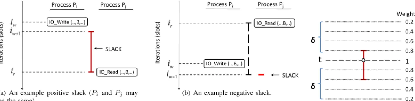
For an access to a disk-resident data (i.e., an I/O call), we define its slackas the distance (measured in terms of loop iterations) between the point at which the data is written into the disk and the point at which data is actually needed (by a read operation). Consider as an example in Figure 6(a). At point iw, process Pi writes data block B into the disk,
and at point ir, B is read from the disk by process Pj.
The region[iw + 1, ir] is termed as the slack for this read
or different. In the former case, we call the slack intra-process slack, and in the latter case, we call it inter-process slack. When read and write operations are from different processes, the read for a particular data block can be issued before the corresponding write, due to loop parallelization and iteration-space normalization. Therefore, a slack can have a negative value, as illustrated by Figure 6(b). In this case, the read needs to wait until the write is done, and consequently, the read can only be issued at point iw+ 1.
As a result, a negative slack becomes a slack of length 1. Clearly, we are interested in positive slacks (i.e., the slacks with a length of more than1 iteration), since they provide us the flexibility of scheduling the access point anywhere betweeniw+ 1andir inclusively.
In our framework, slacks are identified using either the Omega library [23] or the profiling tool. The polyhedral tool is applied when loop bounds and data references are affine functions of enclosing loop indices and loop-independent variables, whereas the profiling tool is used when loop nests are non-affine, or have symbolic bounds. If a loop is very large, to reduce synchronization overhead between the scheduler thread and the application process as well as the running time of our scheduling algorithms described below, we consider d (d > 1) iterations as one unit to measure slacks, instead of 1 iteration.
B. Data Access Scheduling
Once all the slacks in a program are obtained, our data access scheduling step determines a scheduling point within the slack of each data access. In doing so, it considers bothhorizontal reuseandvertical reuseof I/O nodes across data accesses. The horizontal reuse refers to the case where accesses scheduled at the same time from different processes read the data from the same set of I/O nodes, whereas the vertical reuse refers to the situation where accesses scheduled in successive iterations read the data from the same set of I/O nodes. Note that, vertical reuse can happen among the accesses either from the same process or from different processes.
To quantify the I/O node reuse between two data accesses, we define a signature for each access and calculate the
distance between the signatures of these two accesses. Specifically, allnI/O nodes in the target storage architecture are ordered, from the first (number 0) to the last (number (n−1)), and each I/O node is associated with a bit in the signature. Assuming thatDrepresent the set of I/O nodes to be visited by a data access (which can be calculated based on the stripe size), the signaturegfor this access is defined as:g= [η0η1 · · · ηn−2ηn−1], where
ηi=
1, ifi∈ D
0, otherwise.
Theith bit ofg, i.e.,ηi, is1, if I/O nodeiis used by this data
access; otherwise, it is set to 0. Clearly, signatures of two
data accesses tell us a great deal about their similarities as well as their differences. In particular, if two signatures are the same, the corresponding accesses are using exactly the same set of I/O nodes; if the number of different bits between two signatures is n, the two data accesses are accessing disjoint I/O nodes. The distancebetween two signaturesg1
and g2is defined as:
distance(g1, g2) =n−similarity(g1, g2) +difference(g1, g2),
where n is the number of I/O nodes, similarity represents the number of 1s in the same position of two signatures, and differencedenotes the number of different bits. While
similarity captures the number of active I/O nodes that will be reused,differencerepresents the number of additional I/O nodes that will be turned on. Therefore, the distancemetric captures both constraints at the same time, and can be used to maximize the active disk reuse while minimizing the use of inactive disks in successive iterations.
In the following subsections, we first explain a basic scheduling algorithm with assumption that all data accesses (I/O calls) have a length of 1 iteration, i.e., they finish within one scheduling slot, and then extend it to the case in which data accesses are allowed to have different lengths. We also discuss a further modified algorithm that balances two metrics, power andperformance, rather than simply trying to maximize disk power savings.
1) The Basic Algorithm: Given a set of data accesses from different processes along with their slacks, our basic al-gorithm determines the scheduling points for these accesses one-by-one in a nondecreasing order of their slack lengths, starting from the shortest ones. The rationale behind this processing order is that, data accesses with shorter slacks are more constrained compared to those with longer slacks; consequently, it makes sense to schedule them first when considering I/O node reuse. In comparison, data accesses with longer slacks can be postponed without incurring much penalty in most cases, as they have more flexibility.
For a particular access, to determine the ideal scheduling point, we go over all the slots within its slack. If a slot has another access scheduled from the same process, it is considered to be “unavailable” and we skip it. That is, we do not schedule more than one data access in the same slot from the same process. However, data accesses from different processes can be scheduled in the same slot. If a slot is identified as “available”, we then calculate its reuse factor (explained below). After examining all the slots, we select the one with the highest reuse factor as the scheduling point for a data access. If there are multiple slots having the same reuse factor, we randomly choose one of them.
The reuse factorRtfor a slottwithin the slack of a data access is defined by the following two equations:
Rt= k ( 1 dt+k×σ|k|), k∈[−δ, δ] (2) dt+k=distance(g, Gt+k), σ|k|= 1− |k| δ+ 1, (3)
/KͺtƌŝƚĞ ;͕͕͘͘͘͘Ϳ /ƚĞƌ ĂƚŝŽ ŶƐ ;Ɛ ůŽ ƚƐ Ϳ WƌŽĐĞƐƐWŝ ^>< WƌŽĐĞƐƐWũ /KͺZĞĂĚ ;͕͕͘͘͘͘Ϳ
(a) An example positive slack (Pi andPj may be the same). /KͺtƌŝƚĞ ;͕͕͘͘͘͘Ϳ WƌŽĐĞƐƐWŝ ^>< WƌŽĐĞƐƐWũ /KͺZĞĂĚ ;͕͕͘͘͘͘Ϳ /ƚĞƌ ĂƚŝŽ Ŷ Ɛ ;Ɛů Ž ƚƐ Ϳ
(b) An example negative slack. Figure 6. Slack illustrations.
ƚ
ࣦ
ࣦ
ϭ Ϭ͘ϴ Ϭ͘ϴ Ϭ͘ϲ Ϭ͘ϲ Ϭ͘ϰ Ϭ͘ϰ Ϭ͘Ϯ Ϭ͘Ϯ tĞŝŐŚƚƐFigure 7. Vertical reuse range and weight assignment.
where σ|k| denotes the weight, and dt+k represents the distancebetween the signaturegof this access and thegroup active signatureGt+k, which is calculated as:
Gt+k=g(t+k)1|g(t+k)2 |g(t+k)3 |....|g(t+k)m,
where ’|’ stands for the logical bitwise-OR operation, and
g(t+k) represents the signatures of the already-scheduled
accesses at iterationt+k. Clearly, the number (m) of data accesses scheduled at iterationt+k cannot be larger than the number of processes, since only one access from each process is scheduled at any given point.
Note that the reuse factor Rt defined above includes both horizontal and vertical reuses we mentioned earlier. To compute the reuse factor Rt for a slott of a data access, we take into account the reuse between this access and all the other accesses scheduled at iterations betweent−δand
t+δ, where δis a preset (configurable) value, representing thevertical reuse rangewe are considering. The weightσof an iteration in this range is set based on its relative position to the slott. The closer an iteration is to the slott, the higher the weight it gets. Although there are many different ways to assign these weights, we choose to set them according to Eq. 3. For example, if δ= 4, we have σ0 = 1, σ1 = 0.8,
σ2= 0.6, and so on, which means the weights of iterations
t,{(t−1)and(t+1)}, and{(t−2)and(t+2)}, are 1, 0.8, and 0.6, respectively, as shown in Figure 7. Note that, the value ofδ is chosen based on the I/O node characteristics, e.g., the time period required for an idling disk to transition to the low-power mode. The reason is that the disks used between iterationst−δandtmay still be active at iterationt, and similarly, the disks activated at iterationtcan still be in use until iterationt+δis over. In addition, at each iteration betweent−δand t+δ, we consider the horizontal reuse by evaluating the distance dt+k between the signature of
the access being scheduled and the group active signature. However, we use d1
t+k instead of dt+k in Eq. 2, since a
shorter distance represents a better I/O node reuse, which means higher similarity but lower difference as far as the I/O node usage is concerned. Note that,dt+k can be 0, in
which case, d1
t+k is set to2. The pseudo-code of our basic
algorithm is given in Figure 11.
We now illustrate how this algorithm works using ten data accesses from three different processes. Their slacks and signatures on a 16-I/O node storage architecture are given in Figure 8 and Figure 9, respectively. Our algorithm starts with A8, and then processes A6,A3,A5, and so on, based on their slack lengths. Suppose that, the scheduling points (indicated by filled circles in Figure 8) are determined for all accesses except forA4, and now, our task is to find an ideal
scheduling point for it. Based on our discussion above, the slots t4,t7 and t10 will not be considered (as indicated by crosses in the figure), since there are already data accesses (A5,A6,A7) scheduled at these slots from the same process. Consequently, we only calculate the reuse factors for the remaining slots within the slack ofA4, and choose one with
the largest value. Take t6 as an example, to see how to
compute its reuse factor. Assumingδ= 2, we haveσ0= 1,
σ1= 1−1/(δ+ 1)≈0.7,σ2= 1−2/(δ+ 1)≈0.4, and R6=d1 6∗1 + 1 d5∗0.7 + 1 d7∗0.7 + 1 d4∗0.4 + 1 d8∗0.4 = 1 D(g4, G6)+ 0.7 D(g4, G5)+ 0.7 D(g4, G7)+ 0.4 D(g4, G4)+ 0.4 D(g4, G8) = 1 16+ 0.7 20+ 0.7 16 + 0.4 20 + 0.4 14 ≈0.19,
whereDrepresents the distance function, as defined earlier. The reuse factors of other available slots can be calculated in a similar way as follows: R3≈0.17,R5≈0.18,R8≈ 0.22, andR9≈0.19. Based on these values, our algorithm
selects t8 to scheduleA4.
2) The Extended Algorithm: The basic algorithm as-sumed that all data accesses have a length of 1, however, in reality, a data access may take several iterations to finish, depending on the amount of data requested and the time spent in accessing the I/O nodes which hold that data. In the case that data accesses span multiple iterations, we slightly modify our basic algorithm by breaking down each data access into multiple parts (sub-accesses) when calculating the reuse factors.
More specifically, the extended algorithm still sorts the data accesses according to their slack lengths first, and starts with the shortest one. To determine a scheduling point for
ϭ Ϯ ϯ ϰ ϱ ϲ ϳ ϴ ϵ ϭϬ ƚϭ ƚϮ ƚϯ ƚϰ ƚϱ ƚϴ ƚϵ ƚϭϬ ƚϭϭ ƚϭϮ ƚϭϯ ƚϲ ƚϳ dŚƌĞĂĚϭ dŚƌĞĂĚϮ dŚƌĞĂĚϯ /ƚ Ğƌ ĂƚŝŽ ŶƐ ;^ůŽƚƐ Ϳ
Figure 8. An example data access scheduling with lengths of1. Access Signature A1 0 0 1 0 0 0 0 0 0 0 1 0 0 0 0 0 A2 0 1 0 0 0 0 0 0 0 1 0 0 0 0 0 0 A3 0 0 1 0 0 0 0 0 0 0 1 0 0 0 0 0 A4 0 1 0 0 0 0 0 0 0 1 0 0 0 0 0 0 A5 0 0 1 0 0 0 0 0 0 0 1 0 0 0 0 0 A6 0 1 1 0 0 0 0 0 0 1 1 0 0 0 0 0 A7 1 0 0 0 0 0 0 0 1 0 0 0 0 0 0 0 A8 0 0 1 0 0 0 0 0 0 0 1 0 0 0 0 0 A9 0 1 0 0 0 0 0 0 0 1 0 0 0 0 0 0 A10 0 1 0 0 0 0 0 0 0 1 0 0 0 0 0 0
Figure 9. The signatures of the data accesses shown in Figure 8. /ƚ Ğƌ ĂƚŝŽŶƐ ;^ ůŽ ƚƐ Ϳ ƚϭ ƚϮ ƚϯ ƚϰ ƚϱ ƚϴ ƚϵ ƚϭϬ ƚϭϭ ƚϭϮ ƚϭϯ ƚϲ ƚϳ ϭ Ϯ ϯ ϰ ϱ
Figure 10. An example data access scheduling with lengths more than1.
Input: IO accessesA, with the information of beginning
pointa.b, end pointa.e, signaturea.g, and thread IDa.id
for each accessa; Reuse rangeδ, and weightsσkof iterations within this range; Number of total iterationsNt;
Output: A scheduling pointa.pfor eachainA.
1: fori←1 toNtdo
2: Gi= 0; //Initialize the group active signature.
3: end for
4: SortA; //In non-decreasing order (a.e−a.b+ 1). 5: fora∈ Ado
6: BR←0; //Best reuse factor; 7: fori←a.btoa.edo
8: if∃b∈ A& b.p=i&b.id=a.idthen
9: continue; //This slot is unavailable.
10: end if 11: R=distance(1a.g,G i+k)×σ|k| k∈[−δ, δ]; 12: ifR≤BRthen 13: continue; 14: else 15: BR←R;a.p←i; 16: end if 17: end for
18: Ga.p←Ga.p|a.g; //Update the group active signa-ture.
19: end for
Figure 11. The pseudo-code of the basic algorithm.
each access, it goes over all the slots within its slack and eliminates the unavailable ones as in the previous algorithm. However, to calculate the reuse factor of each available slot within the slack of an access, the extended algorithm breaks down all the other accesses into multipleunit data accesses, each of which is assumed to take one iteration, and then computes the reuse factor based on these unit data accesses within the vertical reuse range of the target slot. Since data accesses have lengths now, the vertical reuse range of a target slot t for an access would be iterations betweent−δ and
t+l+δ, where l is the length of that access and δ is a preset value as in the basic algorithm.
We now go over an example, which consists of five data accesses with different lengths in Figure 10, to show how the reuse factor is computed in this extended algorithm. Assume that there are four accesses (A1,A3,A4 and A5)
whose scheduling points have already been determined. In particular, A1 with a length of 12 is scheduled at t1, A3
with a length of4is scheduled att2,A4with a length of6
is scheduled at t3, and A5 with a length of6 is scheduled
att7. Now, we want to determine the scheduling point for the second access (A2) with a length of 3, whose slack
is highlighted using a red line in Figure 10 (from t3 to
t11). Suppose that we are examining the suitability of the
available slott5for this access, and the vertical reuse range
(δ) is2. To compute the reuse factor fort5, we break down
all the other accesses into unit data accesses, as indicated by the unfilled circles in Figure 10. The signature of any unit data access is the same as that of its original access. We then apply Eq. 2 and Eq. 3 to the unit data accesses within the vertical reuse range of t5. Since A2 has a length of 3,
the vertical reuse range of t5 includes the iterations from
t3 to t9. In particular, the weights of t5,t6, and t7 are 1,
the weights oft4 andt8 are 0.7, and the weights of t3 and
t9 are 0.4. The following equation shows the reuse factor calculation ofA2 with respect tot5:
R5= 1 d5∗1 + 1 d6∗1 + 1 d7∗1 + 1 d4∗0.7 + 1 d8∗0.7 + 1 d3∗0.4 + 1 d9∗0.4 = 1 D(g2, G5)+ 1 D(g2, G6)+ 1 D(g2, G7)+ 0.7 D(g2, G4) + 0.7 D(g2, G8)+ 0.4 D(g2, G3)+ 0.4 D(g2, G9),
whereDis the distance function,giis the signature of data
access Ai, and the group active signature Gi is obtained
based on the unit data accesses at iteration ti, e.g., G5 =
g1|g3|g4 andG6=g1|g4.
3) Considering Disk Performance: The algorithms de-scribed so far are designed to achieve the maximum power savings in I/O nodes, without considering performance ex-plicitly, although increasing disk idle periods has an implicit positive impact on performance due to the reduced number of transitions between low-power and active modes. Our observation is that, in some cases, data access scheduling for aggressive power savings may lead to degraded I/O performance. The reason is that such scheduling tends to place a large number of data accesses into the same I/O node within a short period of time, which can in turn cause large queuing delays and reduce the potential parallelism in the I/O subsystem.
To avoid significant performance degradations, we intro-duce a parameter θ into our algorithms, as a threshold to limit the number of data accesses to any I/O node at a time. For example, ifθis set to 2, then at most two accesses (from different processes) to the same I/O node can be scheduled at the same slot. We first show how to accommodate this performance constraint in the basic algorithm presented in
Table I
THE SIGNATURES OF THE DATA ACCESSES SHOWN INFIGURE10.
g1 g2 g3 g4 g5
0 1 1 0 0 1 0 0 0 0 1 0 0 0 0 1 0 0 1 0
Section IV-B1. Instead of picking up the slot with the highest reuse factor, we first sort all the available slots based on their reuse factors in a non-increasing order, and then check these slots one after another, until we find a point (slot) at which all the I/O nodes satisfy the θ constraint. In case that no slot satisfies this constraint, we select the one whose average number of additional accesses to an I/O node is minimum. Assuming that Dt is the set of nodes that have data accesses more than θ at slott and Md represents the
number of accesses to a node d, the average number of additional accesses Et at slottcan be computed as:
Et=
(Md−θ)
| Dt| , d∈ Dt.
For the extended algorithm described in Section IV-B2, a slottis eligible to be the scheduling point for a data access, only if all the iterations fromttot+lmeet theθconstraint, wherel is the length of that access. In addition, to calculate the average number of additional accesses to an I/O node at slot t, we need to consider all the iterations between t
tot+l. Let us consider Figure 10 again, assuming that the data accesses shown are issued to an I/O architecture with
4 nodes, and their signatures gi are as given in Table I. If
θ = 2, then the slot t5 is an eligible point, since at each iteration between t5 and t7, based on the given signatures,
the number of data accesses that target the same I/O node is no more than2.
V. EXPERIMENTALEVALUATION
A. Setup and Methodology
We used the Phoenix compiler infrastructure [6] to im-plement our compiler-based data access scheduling scheme. The longest compilation time recorded during our experi-ments was about 1.4 seconds, which is roughly 40% more than the time taken by the compiler when our scheme is not used. Using the AccuSim simulator [1], we modeled a two-tier storage cache hierarchy, which includes client and server nodes, and each server node maintains a storage cache with I/O prefetching. Our I/O stack includes MPI-IO [39] running on top of the PVFS parallel file system [5]. To model the disks attached to an I/O node accurately, AccuSim interfaces with DiskSim [2], which provides a large number of timing and configuration parameters for specifying disks, controllers and buses for the I/O interface. We augmented DiskSim with detailed power models to keep track of power consumption statistics during different disk operations/states such as seeking, rotation, reading/writing (in different speeds when speed disks are used) and idling. Also, our multi-speed disk implementation models in detail the queuing and
Table II
OUR MAIN EXPERIMENTAL PARAMETERS.
Parameter Value Parameters Common to Spin-Down
Disks and Multi-Speed Disks
Number of Client (Compute) Nodes 32
Number of I/O nodes 8
Stripe Size 64KB
RAID Level 5,10
Individual Disk Capacity 100GB
Storage Cache Capacity 64MB (per I/O node)
Maximum Disk Rotation Speed 12000 RPM
Idle Power 17.1W (at 12,000 RPM)
Active (R/W) Power 36.6W (at 12,000 RPM)
Seek Power 32.1W (at 12,000 RPM)
Standby Power 7.2W
Spin-up Power 44.8W
Spin-up Time 16secs
Spin-down Time 10secs
Disk-Arm Scheduling Elevator
Bus Type Ultra-3 SCSI
Multi-Speed Disk Parameters
Power Model Type Quadratic (See Eq. 1)
Minimum Disk Rotation Speed 3,600 RPM
RPM Step-Size 1,200 Algorithm Parameters δ 20 iterations (slots) θ 4 Table III APPLICATION PROGRAMS.
Name Brief Description Exec Time (minutes)
Disk Energy (Joule)
hf Hartree-Fock Method 27.9 3,637.4
sar Synthetic ApertureRadar Kernel 11.1 1,227.3
astro Analysis of
Astronomical Data 16.8 2,837.6
apsi bution ModelingPollutant Distri- 13.7 3,094.1 madbench2
Cosmic Microwave Background Radiation
Calculation
9.8 1,955.3
wupwise Chromo-dynamicsPhysics/Quantum 39.8 4,812.1
service delays caused by the changes in the RPM of the disks. Our main configuration parameters and their default values are listed in Table II. We later change some of these default values and conduct a sensitivity analysis.
Based on some preliminary experiments, in the simple power-saving strategy, we set the time to wait before spin-ning down a disk to 50 msec (which resulted in good energy savings while limiting the resulting performance penalty to less than 15% for all applications). In the prediction-based strategy, when an idleness is predicted, we selected the corresponding speed such that the maximum performance penalty observed was less than 4%. In the history-based strategy, for each application, we selected the RPM level that bounded the performance degradation by 4% as well. In the staggered strategy, we wait for 50 msec before moving to the next lower speed. Also, we set our defaultδvalue to 20 iterations and defaultθ value to 4.
Table III lists the set of parallel I/O-intensive applications used in this study, which exhibit a variety of data access
patterns. Note that apsi and wupwise are the parallel, out-of-core versions of SPEC applications of the same name [3]. The total sizes of the disk-resident data manipulated by these applications vary between 189.6GB (insar) and 446.1GB (in
wupwise). The third and fourth columns give the application execution times and disk energy consumption values when no power-saving mechanism is employed, which is referred to as theDefault Schemein the rest of our discussion. The energy consumption and performance degradation values presented in Sections V-B and V-C are with respect to this default scheme.
B. Results without Our Approach
We start by presenting, in Figure 12(a), the cumulative distribution function (CDF) of the lengths of the disk idle periods in our applications, when our software-based ap-proach is not used. Specifically, an (x, y%) in this plot means that y% of the disk idle periods have a length of
x msec or less. In applications likehf and madbench,idle periods are very small (more than 90% of the idle periods are less than 50 msec) and therefore very difficult to take advantage of using a conventional spin-down based strategy. On average, one can see that, 86.4% of idle periods have a length of 100 msec or less, and about 96.5% of them have a length of 5 sec or less. Figure 12(c) plots thenormalized
energy consumption values with the four disk-power saving mechanisms explained in Section II when our software-based approach is not used. As expected, the results are not good. First, the simple strategy does not lead to much energy saving (less than 5% on average) since it cannot find many opportunities. In comparison, the prediction-based strategy performs relatively better, generating about 6.3% energy saving over the default scheme. As for the multi-speed disk based strategies, we observe that the history-based strategy ends up saving around 15.6% disk energy, and the staggered strategy leads to an average energy saving of 9.8%. Overall, the history-based strategy generates better energy results than the others.
The performance behavior of these strategies are pre-sented in Figure 13(a). The y-axis gives the performance degradation with respect to the default scheme. Our ob-servation is that the simple strategy causes a significant degradation in performance (10.4% on average). The main reason for this is that this scheme does not adapt its behavior as the length of idle period changes during execution. In many cases, the idle period is short and spin-ups lead to a large impact on performance. To remedy this, one may suggest employing longer waiting periods. However, while doubling the waiting period reduced the performance degra-dation dramatically, it also resulted in less than 1% energy savings, since we could not find any opportunity to spin down disks. Prediction-based and history-based strategies exhibit lower performance degradations since both predict the next idle period. Staggered, on the other hand, incurs a
relatively higher performance penalty since the next access in this strategy can come when the disk has just switched to a very low speed, and the corresponding recovery can be very long in this case.
C. Results with Our Approach
We now quantify the effectiveness of our proposed software-based data scheduling schemes in improving the benefits brought by the underlying disk power-saving strate-gies. Figure 12(b) plots the CDF of disk idle periods when our scheme is used. One can see that the idle times are increased significantly. For example, while in Figure 12(a) the percentage of idle periods with a length of 500 msec or lower was around 90.4%, the periods that fall into the same range constitute about 75.7% of idle periods in Figure 12(b). The impact of these increased idle periods on energy con-sumption and performance are presented in Figures 12(d) and 13(b), respectively. One can observe from Figure 12(d) that, with our approach, the average energy savings for the simple, prediction-based, history-based and staggered strategies are 9.4%, 14.2%, 29.2% and 25.9%, respectively, which are much better than the corresponding (average) savings without our scheme, i.e., 4.7%, 6.3%, 15.6% and 9.8%. Therefore, we can conclude that our approach is very successful in practice. Further, the performance results in Figure 13(b) reveal that our approach is beneficial from a performance perspective as well. For example, the average performance degradation experienced by the simple strategy reduces from 10.4% to 6.9%, and similarly, the history-based strategy experiences a reduction from 1.5% to 1%.
D. Sensitivity Results
We also conduct a sensitivity study by varying the de-fault values of important experimental parameters. In each experiment presented below, the value of only one parameter is changed, and the remaining parameters are maintained at the values given by Table II. We focus on the history-based strategy since the trends with the other strategies were similar, and present the additional energy consumption benefits brought by our approach over this scheme.
The first parameter we experimented with is the number of I/O nodes, and the results are shown in Figure 13(c) (recall that the default value was 8). Our observation is that the energy savings generally increase with increased number of I/O nodes; however, the improvements are not very high. The reason for this is that these results are with respect to the history-based scheme, which already takes an advantage of the increase in the number of I/O nodes. We next changed the value of the δ parameter. Figure 13(d) presents the impact of changing the δvalue while keeping the same weighting strategy explained in Section IV-B1. We see that very small or very largeδvalues reduce our potential energy gains (but for different reasons). Specifically, when
Ϭй ϭϬй ϮϬй ϯϬй ϰϬй ϱϬй ϲϬй ϳϬй ϴϬй ϵϬй ϭϬϬй ϱ ϭϬ ϱϬ ϭϬϬ ϱϬϬ ϭ͕ϬϬϬ ϱ͕ϬϬϬ ϭϬ͕ϬϬϬ ϮϬ͕ϬϬϬ ϯϬ͕ϬϬϬ ϰϬ͕ϬϬϬ ϱϬ͕ϬϬϬн & /ĚůĞŶĞƐƐ;ŵƐĞĐͿ ŚĨ ƐĂƌ ĂƐƚƌŽ ĂƉƐŝ ŵĂĚďĞŶĐŚϮ ǁƵƉǁŝƐĞ (a) Ϭй ϭϬй ϮϬй ϯϬй ϰϬй ϱϬй ϲϬй ϳϬй ϴϬй ϵϬй ϭϬϬй ϱ ϭϬ ϱϬ ϭϬϬ ϱϬϬ ϭ͕ϬϬϬ ϱ͕ϬϬϬ ϭϬ͕ϬϬϬ ϮϬ͕ϬϬϬ ϯϬ͕ϬϬϬ ϰϬ͕ϬϬϬ ϱϬ͕ϬϬϬн & /ĚůĞŶĞƐƐ;ŵƐĞĐͿ ŚĨ ƐĂƌ ĂƐƚƌŽ ĂƉƐŝ ŵĂĚďĞŶĐŚϮ ǁƵƉǁŝƐĞ (b) Ϭй ϮϬй ϰϬй ϲϬй ϴϬй ϭϬϬй EŽƌŵĂůŝnj ĞĚ ŶĞƌ ŐLJ ŽŶƐƵŵƉƚŝŽŶ ^ŝŵƉůĞ WƌĞĚŝĐƚŝŽŶĂƐĞĚ ,ŝƐƚŽƌLJĂƐĞĚ ^ƚĂŐŐĞƌĞĚ (c) Ϭй ϮϬй ϰϬй ϲϬй ϴϬй ϭϬϬй EŽƌŵĂůŝnj ĞĚ ŶĞƌ ŐLJ ŽŶƐƵŵƉƚŝŽŶ ^ŝŵƉůĞ WƌĞĚŝĐƚŝŽŶĂƐĞĚ ,ŝƐƚŽƌLJĂƐĞĚ ^ƚĂŐŐĞƌĞĚ (d)
Figure 12. (a) The CDF of idle periods without our scheme. (b) The CDF of idle periods with our scheme. (c) Normalized energy consumption without our scheme. (d) Normalized energy consumption with our scheme.
Ϭй Ϯй ϰй ϲй ϴй ϭϬй ϭϮй ϭϰй ϭϲй WĞ ƌĨ ŽƌŵĂŶĐĞ ĞŐ ƌĂĚĂ ƚŝŽŶ ^ŝŵƉůĞ WƌĞĚŝĐƚŝŽŶĂƐĞĚ ,ŝƐƚŽƌLJĂƐĞĚ ^ƚĂŐŐĞƌĞĚ (a) Ϭй Ϯй ϰй ϲй ϴй ϭϬй WĞ ƌĨ ŽƌŵĂŶĐĞ ĞŐ ƌĂĚĂ ƚŝŽŶ ^ŝŵƉůĞ WƌĞĚŝĐƚŝŽŶĂƐĞĚ ,ŝƐƚŽƌLJĂƐĞĚ ^ƚĂŐŐĞƌĞĚ (b) Ϭй ϱй ϭϬй ϭϱй ϮϬй Ϯϱй ZĞ ĚƵĐƚŝŽŶ ŝŶ ŶĞƌ ŐLJ ŽŶƐƵŵƉƚŝ ŽŶ Ϯ ϰ ϴ ϭϲ ϯϮ (c) Ϭй ϱй ϭϬй ϭϱй ϮϬй Ϯϱй ZĞ ĚƵĐƚŝŽŶ ŝŶ ŶĞƌ ŐLJ ŽŶƐƵŵƉƚŝ ŽŶ ϱ ϭϬ ϮϬ ϰϬ ϴϬ (d)
Figure 13. (a) Performance degradation without our scheme. (b) Performance degradation with our scheme. (c) Energy reduction as the number of I/O nodes varies. (d) Energy reduction as the value ofδvaries.
disks are still active and tries to reuse them. This can lead to the transition of some disk from the low-power mode to the active mode, which in turn reduces our gains. On the other hand, ifδ is very small, some of the active disks are assumed (wrongly) to be in the low-power mode, and this in turn reduces the flexibility our scheme has in scheduling data accesses, which has an impact on energy consumption. Careful selection of theδvalue is an important issue, which we plan to address in our future work. The energy results with different θ values are given in Figure 14(a). Recall that the θ value limits the number of client nodes that can access the same I/O node in a given scheduling slot, and the default value was 4. We see from Figure 14(a) that, as expected, using a larger value increases our energy gains, but it has a negative impact on performance, as illustrated in Figure 14(b). Like the δ parameter, selection of suitable
θ value is in our future research agenda. We also varied the storage cache capacity in I/O nodes, and observed that, when reducing the cache capacity from 64MB to 32MB, the relative savings our approach brings over the original history-based scheme increased by about 4.3%. In addition, around 3.7% reduction in energy savings was observed when increasing the cache capacity to 256MB. This is because, storage cache itself helped reducing the disk activities, and the larger the cache, the more disk accesses it reduces and the less benefits our approach brings.
VI. RELATEDWORK
One area related to our work is I/O prefetching, which has been investigated by prior studies [29], [12]. Mowry et al [29] present an automatic scheme in which the OS uses
Ϭй ϱй ϭϬй ϭϱй ϮϬй Ϯϱй ϯϬй ZĞ ĚƵĐƚŝŽŶ ŝŶ ŶĞƌ ŐLJ ŽŶƐƵŵƉƚŝ ŽŶ Ϯ ϰ ϲ ϴ (a) Ϭй ϭϬй ϮϬй ϯϬй ϰϬй ϱϬй ϲϬй WĞ ƌĨ ŽƌŵĂŶĐĞ /ŵƉƌ Žǀ ĞŵĞŶ ƚ Ϯ ϰ ϲ ϴ (b)
Figure 14. (a) Energy reduction as the value ofθvaries. (b) Performance improvement as the value ofθvaries.
compiler-provided access pattern information to prefetch. Byna et al [12] propose to use a predetermined I/O signature of an application to guide parallel I/O prefetching. While our work is similar to prefetching in the sense that they both change the original order of data accesses, there are significant differences. First, our approach only fetches the useful data (no speculation) at points within their access slacks. Second, our goal is to reduce disk energy consump-tion rather than hide disk access latencies for performance. Another related area to our work is I/O caching, used for reducing disk energy consumption. Colarelli and Grunwald [17] propose MAID (Massive Arrays of Idle Disks) wherein a small number of disks are used as cache to exploit the locality of I/O requests, while other disks can be spun-down. Zhu and Zhou [45] present two off-line power-aware cache replacement algorithms and two on-line energy-optimal algorithms, namely, PA-LRU [43] and PB-LRU [42]. Our runtime scheduler exploits a similar concept in the sense that it manages a buffer cache to hold the “prefetched”
data. Delay writes [9] and write off-loading [30] are also popular techniques for managing disk power. Samsung [9] announced a flash-based hybrid disk that can delay writes to the magnetic disk by gathering them in the flash buffer and doing a bulk write. Narayanan et al [30] allow write requests on spun-down disks to be temporarily redirected to persistent storage elsewhere in the data enterprise center. These approaches are complementary to both our work and I/O prefetching, since they optimize on I/O writes.
There are also efforts addressing the problem of disk power consumption through software-level optimizations. Weissel et al [40] propose a scheme called Cooperative I/O in which applications can specify deferrable or abortable I/O operations, so that the underlying disk power management can utilize this flexibility to reduce energy consumption. Heath et al increase disk idle periods through application transformations [22]. Papathanasiou suggest using prefetch-ing and cachprefetch-ing strategies to increase the burstiness of I/O access patterns to save power [31], [32]. Pinheiro et al [34] introduce a conservation technique called Popular Data Concentration (PDC) that dynamically migrates the most frequently-accessed disk data to a subset of the disks. Son et al propose several compiler-based code transformations and prefetching techniques to conserve disk energy consumption [37], [36], [38]. Our work is different from these, in that it (i) does not require any code or data layout transformation, and (ii) it schedules data accesses at compile time while selectively issuing I/O requests at runtime.
VII. CONCLUSIONS ANDFUTUREWORK
The main contribution of this paper is a compiler-directed data access scheduling framework developed for maximizing idle periods in parallel applications to reduce disk energy consumption. It contains two components: an optimizing compiler for deciding the data access schedules and a runtime scheduler to prefetch and cache the data according to the schedules. This framework helps avoid extensive code and data layout changes. Our experiments using six application programs reveal that the proposed approach is very effective in reducing disk energy consumption. In the future work, we plan to investigate the opportunities of increasing disk idle periods in multi-application scenarios.
ACKNOWLEDGEMENT
This work is supported in part by NSF grants CNS 1017882, CNS 1152479, CCF 0937949, and CCF 0833126. We thank Prof. Piotr Berman of Penn State for his help in formulating the problem discussed in this paper.
REFERENCES
[1] http://www.mentor.com/products/pcb-system-design/products/accu-sim-2/. [2] http://www.pdl.cmu.edu/DiskSim/.
[3] http://www.spec.org/cpu2006/.
[4] Hitachi deskstar hard drive (P7K500).http://www.hitachigst.com/.
[5] Parallel Virtual File System, version 2.http://www.pvfs.org/.
[6] Phoenix Compiler Infrastructure.
http://research.microsoft.com/en-us/collaboration/focus/cs/phoenix.aspx.
[7] Western digital caviar green hard drive (WD10EACS).http://www.wdc.com/.
[8] Hitachi power and acoustic management - quietly cool. Hitachi White Paper,
2004.
[9] Samsung electronics develops solid state disk using nand flash technology.
http://www.samsung.com/, 2005.
[10] T. Bisson et al. Nvcache: Increasing the effectiveness of spin-down algorithms
with caching.Proc. of MASCOTS, 2006.
[11] T. Bisson et al. A hybrid disk-aware spin-down algorithm with I/O subsystem
support.Proc. of IPCCC, 2007.
[12] S. Byna et al. Parallel i/o prefetching using mpi file caching and i/o signatures.
Proc. of SC, 2008.
[13] E. V. Carrera et al. Conserving disk energy in network servers.Proc. of ICS,
2003.
[14] J. Chase and R. Doyle. Balance of power: Energy management for server
clusters.Proc. of HotOS, 2001.
[15] J. Chase et al. Managing energy and server resources in hosting centers.Proc.
of SOSP, 2001.
[16] G. Chen and others. Compiler-directed channel allocation for saving power in
on-chip networks.Proc. of POPL, 2006.
[17] D. Colarelli and D. Grunwald. Massive arrays of idle disks for storage archives.
Proc. of SC, 2002.
[18] F. Douglis. Thwarting the power-hungry disk. Proc. of the Winter USENIX
Conference, 1994.
[19] F. Douglis et al. Adaptive disk spin-down policies for mobile computers.Proc.
of MLICS, 1995.
[20] E. N. Elnozahy et al. Energy conservation policies for web servers. Proc. of
4th USENIX Symposium on Internet Technologies and Systems, 2003. [21] S. Gurumurthi et al. DRPM: dynamic speed control for power management in
server class disks.Proc. of ISCA, 2003.
[22] T. Heath et al. Application transformations for energy and performance-aware
device management.Proc. of PACT, 2002.
[23] W. Kelly et al. The omega library interface guide.Technical Report, University
of Maryland, 1995.
[24] T. Kenjo.Electric Motors and Their Controls. Oxford University Press, 1991.
[25] E. J. Kim et al. Energy optimization techniques in cluster interconnects.Proc.
of ISLPED, 2003.
[26] K. Li et al. Quantitative analysis of disk drive power management in portable
computers.Proc. of the USENIX Winter Conference, 1994.
[27] W. Liao, K. Coloma, et al. Collective caching: Application-aware client-side
file caching.Proceedings of HPDC, 2005.
[28] Y.-H. Lu et al. Quantitative comparison of power management algorithms.Proc.
of DATE, 2000.
[29] T. C. Mowry et al. Automatic compiler-inserted I/O prefetching for out-of-core
applications.Proc. of OSDI, 1996.
[30] D. Narayanan et al. Write off-loading: practical power management for
enterprise storage.Proc. of FAST, 2008.
[31] A. E. Papathanasiou and M. L. Scott. Increasing disk burstiness for energy
efficiency.Technical report, University of Rochester, 2002.
[32] A. E. Papathanasiou and M. L. Scott. Energy efficient prefetching and caching.
USENIX 04 Annual Technical Conf., 2004.
[33] D. Patterson et al. A case for redundant arrays of inexpensive disks (RAID).
Proc. of ACM SIGMOD Conference on the Management of Data, 1988. [34] E. Pinheiro and R. Bianchini. Energy conservation techniques for disk
array-based servers.Proc. of ICS, 2004.
[35] A. Radding. Energy-efficient storage technologies. SearchDataCenter.com,
2007.
[36] S. W. Son et al. Exposing disk layout to compiler for reducing energy
consumption of parallel disk based systems.Proc. of PPoPP, 2005.
[37] S. W. Son et al. Software-directed disk power management for scientific
applications.Proc. of IPDPS, 2005.
[38] S. W. Son and M. Kandemir. Energy-aware data prefetching for multi-speed
disks.Proc. of Computing Frontiers, 2006.
[39] R. Thakur et al. Data sieving and collective I/O in ROMIO.Proc. of the 7th
Symposium on the Frontiers of Massively Parallel Computation, 1999. [40] A. Weissel et al. Cooperative I/O: a novel I/O semantics for energy-aware
applications.SIGOPS Oper. Syst. Rev., 2002.
[41] P. Zhou et al. Dynamic tracking of page miss ratio curve for memory
management.Proc. of ASPLOS, 2004.
[42] Q. Zhu et al. PB-LRU: a self-tuning power aware storage cache replacement
algorithm for conserving disk energy.Proc. of ICS, 2004.
[43] Q. Zhu et al. Reducing energy consumption of disk storage using power-aware
cache management.Proc. of HPCA, 2004.
[44] Q. Zhu et al. Hibernator: Helping disk arrays sleep through the winter. Proc.
of SOSP, 2005.
[45] Q. Zhu and Y. Zhou. Power-aware storage cache management.IEEE