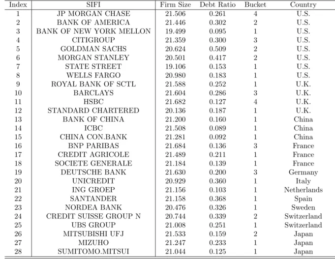
Measuring systemic risk in financial institutions: A factor-copula framework

(1)

Humboldt-Universität zu Berlin School of Economics and Business Ladislaus von Bortkiewicz Chair of Statistics

MEASURING SYSTEMIC RISK IN FINANCIAL

INSTITUTIONS: A FACTOR-COPULA

FRAMEWORK

Master’s Thesis submitted to

Prof. Dr. Cathy Yi-Hsuan Chen Prof. Dr. Wolfgang Karl Härdle

byFlorian Reichert (564471)

in partial fulfillment of the requirements for the degree of

Master of Science in Economics

(2)

Abstract

This work proposes a factor copula model to quantify systemic risk in financial institutions. This framework connects to recently trending research on factor copula modeling and systemic risk measurement. The underlying data are equity returns of the 28 systemically important financial institutions and a common factor which is a portfolio being weighted by these SIFIs. Considering a one-factor copula model with distributional assumptions that enable asymmetric and tail dependence, this framework provides great fit to the underlying financial data. The estimation of the copula density expression is accomplished by the Gauss-Legendre quadratures, a numerical integration and optimization procedure to solve expressions without analytical solutions. Dependence measures and tail dependence coefficients are ob-tained based on the factor copula framework and on a nonparametric approach. Both tail dependence measures, though estimated by a parametric and a nonpara-metric approach, yield results implying a higher tail dependence among the SIFIs in 2015. Then, this work introduces recognized risk measures which become compared in their appropriateness in measuring systemic risk. The focus of the chosen risk measures is to estimates the risk exposure of the financial institutions to the finan-cial system. Hence, the vulnerability of the individual banks is assessed and results indicate again increasing exposure in 2015.

(3)

List of Abbreviations

cdf cumulative distribution function

CDS Credit Default Swap

CoVaR Conditional Value-at-Risk

ES Expected Shortfall

ExCoVaR Exposure∆Conditional Value-at-Risk

GARCH Generalized Autoregressive conditional heteroscedasticity

MES Marginal Expected Shortfall

MLE Maximum Likelihood Estimation

pdf probability density function

PIT Probability Integral Transform

SIFI systemically important financial institutions

(5)

List of Figures

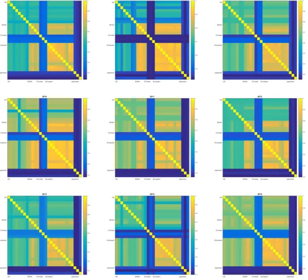
1 Density and scatter plots of the 2008 daily returns of Bank of America, Citigroup, Bank of China, Unicredit and ING Group . . . 30 2 Copula Dependence parameters for the system returns conditional on the

SIFI returns from 2007 until 2015 . . . 35 3 Copula Dependence parameters for the SIFI returns conditional on the

system returns from 2007 until 2015 . . . 36 4 Marginal Expected Shortfall at 95% and 99% quantiles for 2007-2015 . . . 39 5 Empirical Tail Dependence coefficients for the SIFIs for 2007-2015 . . . 43 6 Copula-implied Tail Dependence coefficients for the SIFIs for 2007-2015 . . 44

List of Tables

1 Marginal Parameters . . . 31 2 Summary information on systemically important financial institutions . . . 42 3 Value at Risk at 95% and 99% quantiles for each SIFI . . . 45 4 Expected Shortfall at 95% and 99% quantiles for each SIFI . . . 46 5 Exposure∆CoVaR at 95% and 99% quantiles for each SIFI . . . 47 6 Marginal Expected Shortfall at 95% and 99% quantiles for each SIFI . . . 48

(6)

1 Introduction

What severe consequences does distress in the financial system have on the systemically important financial institutions? Concerning the volatile financial markets over the last decade, in particular the financial crisis and the European sovereign debt crisis, systemic risk has emerged as trending topic among the financial sector and regulators. With re-gards to the Lehman Brothers default and the subsequent turmoil in the banking sector, the interconnectedness of the financial institutions attracted the attention of the public. From then on, large and interconnected financial institutions were seen as systemic risk drivers and the focus of regulators shifted to the arising topics of too-big-to-fail and too-interconnected-to-fail. While the attention of regulators and risk managers moved on to an adequate measuring of systemic risk, dependence and risk measures have been studied in higher frequency.

Risk measures such as Value-at-Risk and Expected Shortfall became criticized for being inappropriate approaches on the quantification of systemic risk born by financial institu-tions. As a result, Adrian and Brunnermeier (2008) and Acharya et al. (2017) introduce risk measures conditional on distressed events. That are the Conditional Value-at-Risk (CoVaR) and the Marginal Expected Shortfall (MES) which hold as more reliable mea-sures of systemic risk. Further research by Mainik and Schaanning (2014) and Girardi and Ergün (2013) extend these measures to address different definitions of systemic risk and to improve their robustness.

Whereas the most common dependence measures concentrate on linear and symmetric dependence and thus yield inadequate estimations during extreme events. Derived from variance-covariance estimation a large number of models belong to the correlation-based approaches which risk quantifications might be an appropriate way under normal mar-ket conditions but lack under non-normal marmar-ket behavior. Since such approaches often assume normality of the risk factors, they misspecify risk by underestimating the depen-dence between risk factors being in a tail event. In Schmidt and Stadtmüller (2006) tail dependence measures have been introduced to capture more adequately pairwise depen-dencies in the tails between financial institutions.

While pairwise dependence measures might not hold as system-wide risk measures that incorporate simultaneous dependencies within high-dimensional applications, the copula function offers a flexible and powerful alternative to traditional dependence coefficients. Joint distribution functions can be decomposed into a copula, containing the entire in-formation set about the dependence structure, and marginal distributions. This

(7)

prop-estimation which essentially enhances the computation due to dimension reduction. In particular when dealing with applications on financial data, the normality and sym-metry assumptions fail to hold. On the basis of financial applications, the normality assumption would rule out the dependence of joint tail events and the symmetry assump-tion would not capture the potentially asymmetric dependence which assigns a higher likelihood to joint downturns than to upturns. While many approaches are fitting copulas to two dimensional models, appropriate copulas which are able to model high-dimensional problems have been revealed by recent research.

Factor models introduced by Krupskii and Joe (2013) became a powerful tool for depen-dence modeling on systemic risk applications. In past literature on factor copula models though (He and Gong, 2009), Gaussian frameworks have been employed frequently due to their attractive feature regarding the estimation of the cumulative distribution func-tion. While heavy tailed distributions are more suitable to capture the characteristics of financial data, they are not stable under convolution and even worse, the distribution does not offer a closed-form solution. Hence, the estimation and corresponding computa-tion require numerical integracomputa-tion and optimizacomputa-tion procedures which distinctly raise the computational efforts and thus create incentives for dimension reduction.

This work addresses this issue by applying a copula model on a factor structure and im-posing heavy tailed distributions. Firstly, the distributional assumption allows for tail dependence within the factor model which secondly, is a powerful tool to reduce dimen-sions being particularly useful for high-dimensional applications. Moreover, factor models only reduce the dimensions for the copula estimation while the marginal distributions are estimated separately within the multi-stage estimation and thus maintain unaffected by the dimension reduction. Oh and Patton (2017a) provide research on dependence model-ing under different heavy tailed distributional assumptions. Extensive research on depen-dence modeling using copulas has been provided by Joe (2014) who applied archimedean copulas on the factor model. Chen and Nasekin (2017) analyzed systemic risk within a network-based factor copula which conditions the network model on a central node which is the most interconnected financial institution. Vrins (2009), Choroś-Tomczyka et al. (2012) and Chen and Nasekin (2017) are based on double t frameworks enabling tail de-pendence.

However, this work proposes a skewed distribution to the systemic factor and hence in-duces asymmetric tail dependence. The structure of the factor model makes the factor copula being solely determined by the distributions for the common factors and the id-iosyncratic components. In this work, the underlying financial data are equity returns of the 28 systemically important financial institutions from pre-crisis period 2007 until

(8)

2015. While the return series of these institutions are used for the idiosyncratic shock, a portfolio weighted by the respective individual sizes represents the common factor. Hence, imposing a heavy tailed and skewed distribution to the systemic factor and a symmetric heavy tailed distributions to the idiosyncratic components results to the desired tail de-pendence and asymmetry which provides a better fit to the financial data.

Once the one-factor structure is introduced, the conditional copula expression is derived after applying an uniform transformation method. While this work considers a Maximum likelihood estimation for the copula density, Oh and Patton (2013) propose the simulated method of moments estimation method to factor copula models which do not provide closed-form solutions. Since many heavy tailed copula frameworks are not solvable ana-lytically, the likelihood expression must be obtained by the means of numerical integration methods. Thereby, quadrature methods are presumed to yield adequate results. Whereas Vrins (2009) applied Gauss-Hermite quadratures, which sometimes lack of bounded ap-proximation errors, Gauss-Legendre quadratures address this issue and are employed by Oh and Patton (2017b) and Chen and Nasekin (2017). Then, the resulting simulated returns are the underlying series for the estimations of the risk measures. Thereby, after obtaining the popular measures of VaR and ES, this approach will focus on the vulnera-bility of each financial institution to the financial system and hence takes the Exposure CoVaR approach by Adrian and Brunnermeier (2008) and the Marginal Expected Short-fall by Acharya et al. (2017) into account. This setting then focuses on the event when a system-wide shock occurred and investigates the subsequent impact on all financial in-stitutions based on a simultaneous analysis. Hence, this work follow up to the analysis of existing research which studied the systemic risk born by institution-specific extreme tail events and the resulting effect on the financial system. This has been studied by, among others, Girardi and Ergün (2013), Mainik and Schaanning (2014), Cao (2013) in a multivariate framework and Chen and Nasekin (2017) in a network-based factor copula model .

While this work tries to quantify the systemic risk in financial institutions, it examines dependences structures within the financial system and tail dependencies between the banks themselves at first and continues to assess the appropriateness of the proposed risk measures. The dependence within the financial system increases during more volatile periods as it is implied by the distributional assumptions. Though, results for the most recent year 2015 show higher dependence again, indicating an increasing interconnected-ness in the financial system after periods of decreasing dependence structures. In order to the factor copula parameters and the tail dependence coefficients, clustered dependencies

(9)

from the Asian financial sector on the overall and in particular Western banking sector. In line with the results on dependencies, the risk measures also yield comprehensible findings marking crisis periods quite well while they also identify higher individual systemic risk exposure of all institutions to the financial system in 2015. Thereby, the conditional risk measures obtain some results that are not yielded by the simple risk measures of VaR and ES which can be traced back to the different nature of the risk measurement approaches, such as conditioning on a stressed system. Anyway, the broad consistency of the risk estimates’ and the dependence measures’ results does not only lead back to the common model-approach on which the estimates are based on since even the nonparametric tail dependence supports the other estimates and suggests a higher interconnectedness within the financial system in 2015.

The structure of this work is constructed as follows. In section 2 basic theory on copulas, dependence measures and factor model are presented to continue with the construction of the factor-copula framework. This section on the methodological background is followed by the estimation part 3 which applies the Maximum Likelihood estimation method to ob-tain a solution to the copula density estimation. While this framework assumes heavy tail distributions on the one-factor copula increments, the Maximum Likelihood estimation requires numerical integration and optimization methods to achieve a solution. Hence, the subsequent section 3.2 deals with the methodology, computational implementation and existing research applications on numerical solution methods. Then, the work turns to the section 4 that discusses the adequacy of prevalent risk measures for estimating sys-temic risk in financial institutions. Finally, the results section 5 presents useful estimates to dependencies within the financial system and compares the risk measure estimates in the course of their appropriateness in quantifying systemic risk and according to their vulnerability to a shock of the financial system.

(10)

2 Methodology

This chapter is constructed as follows. First, basic concepts on copula and dependence measures are introduced. The main part of this chapter deals with the factor copula model, the implementation of the distributional assumptions and the derivation of the copula density function.

2.1 Theory on Copula

Consider for the d-variate stochastic process Y n_t₌₁ with Yt = (y1,t, ..., yd,t) the joint

distribution F(y1,t, ..., yd,t) and the corresponding marginal distribution Fi and density

function fi of each variable yi,t.

By Sklar’s Theorem (Sklar, 1959) the joint distribution can be expressed by thedmarginal distributions which are "coupled" together by a copula function. A d-dimensional copula is a function C from [0,1]d _→ _[0_,_1] _{that contains all information about the dependence}

structure. Hence,

F(Yt) = C(F1(y1,t), ..., Fd(yd,t)) (1)

Thereby, the copula can be seen as a multivariate distribution function linking marginal distributions F1, ..., Fd to the joint distribution F. Sklar’s Theorem provides following

practical properties. Firstly, using the given univariate distributions F1, ..., Fd and a

cop-ula C, the theorem allows for the flexible construction of joint distributions F. Secondly, Sklar’s Theorem enables multi-stage estimation which considerably lower the computa-tional efforts when dealing with high-dimensional problems. The copula estimation con-sists of the estimation of the copula parameters θC and the margins Fi, i = 1, ..., d.

Depending on the practical application, the maximum likelihood estimation of the mar-gins can be accomplished in a non-parametric model, which is in particular appropriate if the focus is only on the dependence structure, or in a parametric model. Latter one is more often applied in practical problems in which the entire distribution is of relevance. When applying the nonparametric approach, the maximum likelihood (ML) estimator should be proven to yield consistency and asymptotic normality. Within the parametric procedure, the ML estimation can be accomplished simultaneously for the parameter esti-mation of the margins and of the copula. This simultaneous (one-stage) estiesti-mation is more efficient than any multi-stage estimation procedure but brings an higher computational burden for high-dimensional applications (Genest et al., 1995). Thus, this framework applies the computationally attractive parametric two-stage estimation in which the

(11)

pa-Assuming an arbitrary continuous multivariate distribution which can be modeled para-metrically, the probability integral transform (PIT) can be applied on equation (1) by imposing ui,t = Fi(yi,t;θm,i), where ui,t ∼ U nif orm(0,1) and θm,i is the vector for all

parameters of margin i. Then, δ is the vector of all marginal parameters fori = 1, ..., d. Since copulas are invariant under strictly increasing transformations, the PIT used on the random variables does not affect the copula functions.

C(u1, ..., ud) = F(F1−1(u1), ..., F_d−1(ud)) (2)

where F_i−1 is the generalized inverse of Fi. Hence, the copula can be described as a

multivariate distribution with uniform margins and by considering the uniform transforms for equation (1), the copula density becomes:

c(u1,t, ..., ud,t) =

∂d_C₍_u

1, ..., ud)

∂u1...∂ud

(3) Under the assumptions of a continuous multivariate distribution and a parametric model, one can also assume by Sklar’s Theorem and by mixture families models the univariate marginal distribution and the copula to be continuous and parametric. Hence, equation (1) and (3) can be written as (Franke et al., 2004):

f(Yt) = d

Y

j=1

fi(yi,t)·c(u1,t, ..., ud,t) (4)

where f represents the joint density of Yt. According to equation (4) which consists only

of marginal densities fi and the copula on the right hand side, it becomes obvious that

the copula provides all information regarding the dependence structure.

2.2 Tail Dependence Properties

There are several approaches on the definition of pairwise dependence in random vari-ables. The most common measures reflect linear and symmetric dependence or consider the entire distribution. In contrast, dependence can also be defined to be asymmetric, nonlinear or only consider the tail distribution. Thereby, dependence can be measured in an empirical way or model-implied (Chen and Nasekin, 2017).

When models with flexible dependence structures are employed, the linear correlation measure which is natively used under the multinormal assumption needs to become aug-mented by other dependence measures. The commonly employed linear correlation co-efficient is not scale invariant and changes due to monotone increasing transformations.

(12)

That is the case because linear correlation is affected by the marginal distribution while in a copula framework appropriate dependence measures should only depend on the cop-ula. Due to this property these measures provide information about the degree to which random variables gather around a monotone function (Joe, 1990).

That is why, an adequate dependence measure for a copula model is scale invariant (see Nelson 2006) and independent of strictly increasing transformations of the random vari-ables such as the probability integral transformation which is described earlier in this framework. Following simulated rank dependence measures are common augmentations on the linear correlation since they are functions of the copula only (Patton et al., 2012). Therefore, consider the copula framework with two random variables yi,t and yj,t, their

corresponding marginal distributions Fi and Fj and the copula C.

Spearman’s rank correlationbetween random variables is measured by using the vari-ables’ concordance and discordance and can be considered as the linear correlation of the ranks of the simulated data. The population rank correlation ρ can be written as:

ρ=Corr(ui,t, uj,t) = 12E(ui,t, uj,t)−3

= 12 Z 1 0 Z 1 0 C(ui, uj)duiduj−3

where _E(u) = 1/2 and _V(u) = 1/12for any random variable u ∼ U nif orm(0,1). Then, the sample rank correlation ρˆcan be estimated as:

ˆ ρ= 12 n n X t=1 ui,tuj,t−3

Kendall’s taubetween random variables is obtained by the difference in the probabilities of concordance and discordance. The Kendall’s tau is calculated by:

τ = 4_E(C(ui,t, uj,t))−1 = 4 Z 1 0 Z 1 0 C(ui, uj)dC(ui, uj)−1

As Spearman’s and Kendall’s rank correlation coefficients are defined in the interval [-1,1] the direction of the dependence is given. These both measures may offer the most suit-able alternatives to the linear correlation measure when dealing with dependence for non-elliptical distributions (Embrechts et al., 2001).

(13)

ability of one variable being in the q-th quantile conditioned that the other variable is is in the q-th quantile. On the one hand, while obtaining the lower and upper quantile dependence, information about the symmetry of the dependence structure are provided. On the other hand, this measure is defined in the interval [0,1] and thus, only shows the degree of dependence but tells nothing about the direction as the previous coefficients do (Patton et al., 2012).

Tail dependence is besides Quantile dependence another dependence measure of ex-treme events. This approach focuses on the upper-right and lower-left quadrant tail of a bivariate distribution of two random variables and therefore it measures the strength of dependence in the tails of a bivariate distribution. Since this analysis focuses on measur-ing risk in the financial markets under severely adverse market conditions the lower tail dependence coefficient is of higher relevance. In general, the tail dependence is defined by: τ_ijL ≡lim q→0 PhXi ≤Fi−1(q), Xj ≤Fj−1(q) i q (5) τ_ijU ≡lim q→1 PhXi > Fi−1(q), Xj > Fj−1(q) i 1−q (6)

The lower tail dependence gives the probability that both variables are below their q quantiles scaled by the probability of one of these variables being below its q quantile for the lower bound q →0(Oh and Patton, 2017a).

Hence, equation (5) and (6) are the limits of the quantile dependence and by embedding them into a copula framework it takes following form (De Luca and Rivieccio, 2012):

τ_ijL= lim q→0 C(q, q) q (7) τ_ijU = lim q→1 1−2q−C(q, q) 1−q (8)

Whereas the majority of factor-copulas have no closed-form solution, the copula-implied tail dependence coefficients can be obtained in an analytical way utilizing results from extreme value theory. Based on the simple linear framework of a factor model the results for the copula-implied dependence are easy to calculate. Consider the one-factor copula model from equation (14) and under the assumptions that FZ and F have regularly

varying tails with a common tail indexα >0and that the copula parameter of each SIFI bank θ >0 holds, the tail dependence coefficients are given by equation (9) and (10).

τ_ijL= min(θi, θj)

α_AL Z

min(θi, θj)αALZ+ALε

(14)

τ_ijU = min(θi, θj) α_AU Z min(θi, θj)αAUZ +AUε (10) where AL

Z, AUZ,ALε and AUε are constants which are given by the respective distributions.

Since the implied tail dependencies are conditioned on a selected factor, they are also named conditional tail dependencies. In this case, the tail dependencies are conditioned on the systemic factor Z. Note, that the selections of the conditioning factor and the copula mainly determine the final tail dependencies (Chen and Nasekin, 2017).

According to the factor copula model from equation (14) lower and upper tail dependence coefficients are obtained if the sign of the copula parameters and the tail index of Z and ε are the same. The tail dependencies will be different and thus, enables to model different probabilities of joint market up and down if FZ or Fε is asymmetric (Oh and

Patton, 2017a). Applying a non-normal distribution to the model from equation (14), the systemic factor may have less weight on the upper tail than on the lower tail whereas ε is symmetrically distributed (tail index of ε equals lower tail index of Z). Then, the upper tail dependence from equation (10) equals zero and the lower tail dependence from equation (9) is positive.

Referring to the one-factor copula model from equation (14), FZ = Skew t(ν, λ) and

Fε =t(ν), the tail indices of Z and ε equal the degrees of freedom ν and the constants

from equation (9) and (10) can be calculated as follow:

AL_Z = bc ν b2 (ν−2)(1−λ)2 −(ν₂+1) , AU_Z = bc ν b2 (ν−2)(1 +λ)2 −(ν₂+1) AL_ε =AU_ε = c ν 1 ν−2 −(ν₂+1)

where the parameters of the defined distribution are used for a = 4λc(ν −2)(ν −1), b =√1 + 3λ2₋_a2 _and _c_{= Γ(}ν+1

2 )/(Γ(

ν

2)

p

π(ν−2)) (Oh and Patton, 2017a).

Apart from the copula-implied tail dependence measures above, the tail dependencies can also be obtained with a non-parametric approach. These measures are widely known as the empirical tail dependence coefficients. Schmidt and Stadtmüller (2006) propose to estimate the coefficients by two nonparametric estimation methods, either by using the empirical tail copula or based on the stable tail-dependence function. Since these non-parametric estimators apply empirical distribution functions to model the marginal distributions, it circumstances the lack of possible misidentification arising from a wrong parametric specification. The non-parametric fit provides also more flexibility by dropping

(15)

the restrictive fashion of a parametric model. ˆ τ_ijL:= n kC kxi n , kxj n ≈ 1 k n X t=1 I(R(_it)≤kxi, R (t) j ≤kxj) (11) ˆ τ_ijU := n k ˜ C kxi n , kxj n ≈ 1 k n X t=1 I(R(_it) > n−kxi, R (t) j > n−kxj) (12)

whereC˜ is the empirical survival copula withF˜i = 1−Fi,k is a threshold parameter and

R denotes the rank of the underlying data x. The very right sides in equation (11) and (12) show in an approximative framework two rank-order-statistics based on a modified empirical tail copula. Further details can be found in Schmidt and Stadtmüller (2006).

2.3 The factor copula model

Portfolio models can be distinguished between reduced form models and structural models to which factor models belong. Factor models have become frequently applied in several sciences. These models can capture agent’s shared behavior through joint common fac-tors. When combining variables to a lower number of common factors, factor models are powerful tools for dimension reduction. Moreover, factor copulas models outperform other copula classes in terms of their high usefulness for copula parameter estimation under the curse of dimensionality and time complexity. Introduced by Krupskii and Joe (2013) factor copulas are explained as a copula framework applied on a factor structure which enhances high-dimensional estimations and lowers the computational burden due to a reduced number of parameters (Krupskii and Joe, 2013). This more flexible model set-ting allows to fit dependence structure more adequately than linear dependence measures since the copula framework can serve for non-linear and varying dependence structures among the variables and the common factors.

In general, the multivariate factor copula model presumes a linear dependence structure of d observed variables Z on pconditional factors W:

Zi = p

X

k=1

αi,kWk+εi (13)

where W ∼iid FW(γW), εi ∼iid Fε(γε)and Wk⊥εi ∀i, k based on d+p latent variables

(Oh and Patton, 2017a). Thereby, the common factorsW are assumed to be independent and identically distributed. The independence assumption is required by the numerical optimization procedure when estimating the copula density in section 3. The latter as-sumption simplifies the estimation by reducing the number of parameters being obtained

(16)

by the numerical integration method. Moreover, the parameters of the common factors’ distributions are assumed to be equal to further mitigate the numerical integration efforts. However in this work, the factor model from equation (13)(Krupskii and Joe, 2013) re-duces to one factor p= 1:

Zi =αiW +

q 1−α2

iεi (14)

where all assumptions on the distributions FW and Fε from the multiple factor case of

equation (13) stay valid and the vector of the factor copula parameters is defined as θC = (α1, ..., αd, γW0 , γ

0

ε). Now, in order to construct the copula and without any loss of

generality, the margins are defined as i.i.d. random variables and follow U nif orm(0,1). Hence, the random variables Zi are transformed to conditionally independent uniform

random variables ui ≡ FZi(Zi) given the uniform representation of the common factor

v ≡ FW(W). Then, using Zi = F_Zi−1(ui) and applying the factor model on the copula

function from equation (2), the factor copula writes as follows: CV(u1, ..., ud) = F(Z1, ..., Zd) = Z 1p 0 FZ|v1,...,vp(Z|v1, ..., vp)dFv(v1)...dFv(vp) (15)

where FZ|V represents the conditional joint cdf of the vector U on the vector V. After

transforming the p independent variables to uniform random variables, any conditional independence model is able to fit this form. Considering the univariate factor case p= 1

and under the assumption of independent U ≡(u1, ..., ud)T, it follows:

Cv(u1, ..., ud) = Z 1 0 d Y i=1 FZi|v(Zi|v)dFv(v) = Z 1 0 d Y i=1 CFZ(Zi)|v(FZ(Zi)|v)dv = Z 1 0 d Y i=1 Cui|v(ui|v)dv (16)

Sinceui, v are uniform random variables andCui,v andcui,vare their joint cdf and density,

it holds that Fui|v(ui|v) = Cui|v(ui|v) =

∂C_ui,v(ui,v)

∂ v which is used to derive the second

equation above. Equation (16) denotes the factor copula model consisting of a sequence of bivariate copulas which link the random variables ui to the common factor v. Noting

that ∂ Cui|v(ui|v) ∂ui =

∂2_C

ui,v(ui,v)

(17)

the one-factor copula density becomes: c(u1, ..., ud) = Z 1 0 d Y i=1 cui,v(ui, v)dv (17)

According to equation (4) all information about dependence are solely explained by means of the copula density that due to the just derived one-factor copula equation (17) consists of d bivariate linking copulas. More details can be found in Krupskii and Joe (2013). Now, the conditional pair copula will be derived from equation (16) and using the factor structure from equation (14):

Cui|v(ui|v) =Fui|v(ui|v) =Fεi F_Zi−1(ui)−αiFW−1(v) p 1−α2 i ! (18)

which is the general expression for the conditional independence structure of the uni-form margins within the factor model. That is, ui are independent with conditioning

variable v (McNeil et al., 2015). Based on the one-factor model from equation (14) the dependence structure can be modeled in various ways depending on the distributions of the common factor W and the idiosyncratic component ε. Note that the copula is only given in closed form solution for FW and Fε being normally distributed. The resulting

multivariate normal distribution has been used by Lu et al. (2015) and Krupskii and Joe (2013). The closed form solution for normally distributed random variables is a Gaussian copula. Thus, the dependence structure is determined by the choices of distributions for W and ε.

Choosing instead heavy tail distributions and an asymmetric one for the common factor enable tail and asymmetric dependence which will be useful for the later analysis. A t-copula, for instance, enables joint heavy tails and a higher probability of joint extreme events in comparison to a Gaussian framework. Oh and Patton (2017a) provided exten-sive research on factor copula models and show the high degree of adaptability of this copula class by using normal, t and Skew t marginal distributions to model different de-pendence structures such as asymmetric and tail dede-pendence. Chen and Nasekin (2017) applied a double-t copula to a network-based factor model. In contrast to the Gaussian copula framework, heavy tail and asymmetric factor copulas do not provide a closed form solution. Considering such distribution for parameter estimation on equation (18), the solution for distribution FZi is then to compute numerically via convolution of αiW and

p 1−α2

iεi (Chen and Nasekin, 2017). According to Borak et al. (2011), the double

(18)

normal inverse Gaussian copula framework modeled by Kalemanova et al. (2007), which both belong to the class of generalized hyperbolic distributions, yield the best fit for finan-cial data. However, modeling tail dependence with generalized hyperbolic distributions demands restrictive assumptions on the parameters. Apart from the parametric family of elliptical copulas, Archimedean parametric copulas have been analyzed in factor settings by recent research from Granger et al. (2006), He and Gong (2009) and Shamiri et al. (2011) who studied approaches on Gumble, Clayton and Frank copulas. Although, these Archimedean copulas have the properties of tail dependence and asymmetry and hence provide a possibly good fit to financial data, they are quite restrictive in high-dimensional frameworks. That is because the dependence between all random variables can only be determined by one or two parameters.

This work considers the Skew t−t factor copula proposed by Oh and Patton (2017a) in order to enable tail dependence and asymmetry and to provide a good fit to the data. The financial data are stock price returns of 28 banks which are weighted according to the banks’ sizes to construct a system portfolio as representation of the common factor. To obtain a measure for systemic risk driven by idiosyncratic risk, the returns of each bank yi,t are approximated by a GARCH(1,1) model to isolate the idiosyncratic

compo-nent. This component is cleaned from the GARCH effect by using each bank’s zero mean returns to exclude the market impact and by standardizing the distribution within the GARCH(1,1)framework (Fantazzini, 2008):

yi,t =ai+biym,t+εi,t (19)

h2_i,t =ωi+βihi,t2 −1+αiε2i,t−1 (20) Zi,t = r _ν i h2 i,t(νi−2) εi,t ∼tνi,λi (21)

where firstly, in the upper equation the bank-specific returns are regressed on the market returns. Secondly, the regressions’ residuals are controlled for the GARCH effect with one lag for both elements, the autoregressive and the conditional variance part. Thus, the obtained idiosyncratic residual returns and the systemic residual returns are presumed to be iid random variables following a standardized t and a Skew t distribution (Chen and Nasekin, 2017). The respective variances within the factor copula model are set to one (Oh and Patton, 2017a). Tail and asymmetric dependence are ensured by applying a Skew t−t factor copula model.

(19)

First of all, the Skew t density is presented (Hansen, 1994): f(W|ν, λ) =          bc 1 + 1 ν−2 bz+a 1−λ 2 −ν+1₂ z <−a b bc 1 + _ν₋1₂ bz₁₊+_λa2 −ν+1₂ z ≥ −a b (22) where a= 4λc ν−2 ν−1 , b2 = 1 + 3λ2−a2, c= Γ( ν+1 2 ) p π(ν−2)Γ(ν₂) (23) Γ is the gamma function and the parameters of the t distribution are given by ν and λ which are the degrees of freedom and the skewness parameter, respectively. By definition, it holds thatν ∈(2,∞)and λ∈(−1,1). TheSkew t distribution has mean zero and unit variance. For increasing degrees of freedomν, the distribution approximates to the normal distribution and the probability of extreme co-movements decreases. The density function is left-skewed for λ < 0, symmetric forλ = 0 and right-skewed for λ >0. For λ = 0and ν 6= +∞ it becomes the standardizedt distribution and for the extreme case of infinitely large degrees of freedom the t distribution converges to the normal distribution. Keeping ν = +∞ but having non-zero skew λ6= 0 it renders in a skewed normal distribution. For the sake of simplicity, the degrees of freedom are equal forW andεiand are determined

by the systemic factor. Hence, for a Skew t− t copula model with underlying factor structure of equation (14) and equalνforFW andFεrequires to estimated+2parameters.

That is, d copula parameters and one degree of freedom and one skewness parameter. Then, equation (2) gives the multivariate t-copula of the multivariate t-distribution:

C_νt(u1, ..., ud) =Tνd(T

−1

1 (u1), ..., Td−1(ud)) (24)

where T_νd is the multivariate t-distribution and T_ν−1 is the inverse univariate cumulative distribution function.

The pair copula representation in equation (18) comes from the specific case of a Gaussian copula framework in which the derivation is independent from the factor copula parameter α and hence in a Gaussian framework αdenotes nothing more than the linear correlation coefficient (Krupskii and Joe, 2013). This is given by the convolution stability of the Gaussian function. The solution to the Gaussian pair copula formulation would then result analytically since the sum of two Normal variables gives a Normal variable again. While for the Gaussian formulation (14) remains the same, this simple representation does not hold anymore in this Skew t−t model though and the distribution is neither stable under convolution nor provides any analytical solution. The distribution then becomes

(20)

a weighted sum of two unit-variance t-distributed random variables which need to be standardized such as W =. W(ν) q ν−2 ν and εi . = εi(ν) q ν−2

ν for a double t model. Vrins

(2009), Kolman (2014) and Choroś-Tomczyka et al. (2012) express the conditional pair copula distribution for a double t one-factor model as follows:

Cui|v(ui|v) = Tν " Zi−αi q ν−2 ν W q 1−α2 j q ν−2 ν # (25)

where Zi = Tν−1(ui) and W = T_ν,λ−1(v). Furthermore, with respect to the skew, Chan

and Kroese (2010) present a one-factor copula model expression for a Skew t−t model. The Skew t -t model within a factor copula framework can also be expressed in terms of W ∼iid N(0,1)and εi ∼iid N(0,1):

Zi = αiW +λS+ q 1−α2 iεi η−1 (26) with S ∼T N − r 2 π,1 (27) whereT N(µ, σ2)is a truncated normal distribution with left truncated mean−q2

π. λ >0

then includes the right-skewed property to the distribution and η−1 _{is nothing more than} a mathematical construct that brings the t-distributional property into the model such that η2 _∼_Γ(ν

2,

ν

2). Anyway, this component can also be understood as shock term which triggers many simultaneous defaults for smallη. This setting under a doubletframework is also considered by Franke et al. (2004) and Chan and Kroese (2010). Due to the setting of equation (26), Chan and Kroese (2010) show that the distribution ofZi becomes

asymmetric and the skewness is induced by the parameterλwhereas the mean ofZi is not

affected by the term λS. Oh and Patton (2017a), Embrechts et al. (2005) and Lin et al. (2013) however suggest to include the skew into the factor representation from equation (14) such as: Zi =αi r ν−2 ν W +λ r ν−2 ν S˜+ r (1−α2 i) ν−2 ν εi (28)

where S˜ = _Vν is scalar independent of W with V ∼ χ2_ν and thus S˜∼ Inv χ2_ν (Embrechts et al., 2005).1 _{Due to this simple formulation in equation (28) the double} _t _{copula model}

becomes generalized to allow for an asymmetric distribution triggered by the skewness

(21)

parameter λ (Chan and Kroese, 2010). Applying the distributional assumptions on the one-factor structure of equation (28) with normal margins, the conditional copula (25) becomes: Cui|v(ui|v) =Tν " Zi−λ q ν−2 ν S˜− q ν−2 ν αiW q 1−α2 j q ν−2 ν # (29) By equation (16) and (29) it follows:

Cv(u1, ..., ud) = Z ∞ −∞ d Y i=1 ( Tν " Zi−λ q ν−2 ν S˜− q ν−2 ν αiW q 1−α2 j q ν−2 ν #) tν(W)dW (30)

For the sake of simplicity, the following sections will stick to the expression introduced by equation (14) to represent the Skew t−t model under the distributional assumptions of W ∼ iid TW(ν, λ), εi ∼iid Tε(ν)where W ⊥ εi∀i, k. Therefore, Frey and McNeil (2001)

also use the simplified setting of an exchangeable one-factor model for various distribu-tions. Hence, for the further analysis, the equation (18) is used. This representation for a Skew t-t framework is also chosen by Yang et al. (2009) and Oh and Patton (2017a) who use an exchangeable one-factor model representation for the sake of comparison between the different distributional assumptions in their extensive work on factor copula models. Azzalini and Capitanio (2003) also apply the notation of the one-factor copula model structure from equation (14) on skewed elliptical distribution frameworks. Bluhm and Wagner (2011) employ a mixed distribution approach on the same one-factor model for-mulation.

The equation (30) has, as already stated above, no closed form solution and the model implementation is mainly dependent on an accurate integral computation. The copula pa-rameters are estimated by maximum likelihood estimation employing the Gauss-Legendre quadrature for numerical integration for the copula density estimation. The next section will enlarge upon the factor copula density estimation by numerical integration method.

(22)

3 Estimation of the factor copula model

In general, the estimation of a multivariate distribution based on a copula can be ac-complished in only one step that includes the estimation of the copula parameters θC

and the estimation of the margins Fi with i= 1, ..., d. However, as mentioned in section

2.1, Sklar’s Theorem also allows for multi-stage estimation which provides advantages for the computation in terms of high-dimensionality. The applied maximum likelihood estimations furthermore can be embedded in parametric and nonparametric models for the margins. Thereby, the entire distribution is considered for parametric models, that are the full maximum likelihood estimation and the inference for margins method which are one-step and two-step procedures, respectively. The one-step simultaneous estima-tion procedure achieves consistent and efficient estimators but calls for high numerical complexity under high dimensionality since the simultaneous method jointly estimates the marginal and the copula parameters. Semi- and nonparametric estimation methods for the margins are quite suitable if the interest is merely on the dependence structure and to avoid a parametric restriction to the unknown marginal distributions. Then, the multi-stage semiparametric method, that is the pseudo maximum likelihood, also canon-ical maximum likelihood, obtains nonparametric estimates for the marginal distributions by applying empirical distribution functions and thus, enables the estimates to be inde-pendent of restrictive parametric families. After that, the dependence structure between the margins is obtained by using a parametric copula estimation for the uniformly trans-formed pseudo sample (Kim et al., 2007). As shown by results of Genest et al. (1995) the simultaneous estimation of the full maximum likelihood is preferred over two-stage solutions, although the pseudo maximum likelihood estimator becomes consistent and asymptotically efficient under certain conditions.

In this framework, the estimation of the factor copula model is carried out with a multi-stage maximum likelihood that requires the log-likelihood function of the one-factor cop-ula model to become decomposed into two components. This is necessary to enhance the computational performance in high-dimensional problems. Next the estimators are presented before the standard errors will be obtained. Finally, a numerical integration and optimization procedure for maximum likelihood is applied to achieve an expression for the factor copula density (17). Thereby, the estimation of the cumulative distribution function proceeds the inverse distribution function estimation which can be calculated af-terwards numerically (Vrins, 2009). Now, suppose under the copula density from equation (17) belongs to a parametric familyC ={Cθ, θC ∈ΘC} and considering equation (4) and

(23)

L(y1, ..., yn;θ) = n

Y

t=1

f(y1,t, ..., yd,t;θm,1, ..., θm,d, θC) (31)

Now, the likelihood function (31) must be decomposed into two components, the likelihood contributions from the marginal distributions and from the dependence structure (Choroś et al., 2010). The decomposed log-likelihood function is given by:

l(y1, ..., yn;θm, θC) =lm(θm) +lC(θC, θm) (32)

which can be rewritten as:

l(y1, ..., yn;θm, θC) = n X t=1 d X i=1

log fi(yi,t;θm,i)

+ n X t=1 log c(F1(y1,t; ˆθm,1), ..., Fd(yd,t; ˆθm,d);θC) (33)

where the estimation of the parameters for the uniform margins takes place at first stage and for the copula parameters at second stage with the marginal parameters fixed at the estimates from the first estimation stage. The log-likelihood for the marginal distributions is further decomposed into d log-likelihood expressions for d margins. The resulting estimates for θm are required for the copula parameter estimation since the probability

integral transforms are derived using the marginal parameters. The first stage estimation to obtain the d parameters of the marginal distributions is given by:

ˆ

θm,i = argmax θm,i

lm,i(θm,i) (34)

The factor copula density in the second stage has no analytical solution for the distri-butional assumptions made in this framework. Hence, the log-likelihood of the copula model is solved via a numerical integration method which will be discussed later in sec-tion 3.2. Given the estimated marginal parameters θˆm = (ˆθm,1, ...,θˆm,d)0 the dependence

parameters solve the pseudo log-likelihood function lC(θC,θˆm)at second stage:

ˆ

θC = argmax θC

lC(θC,θˆm,i) (35)

Except for the particular case of a multivariate Gaussian copula with normal marginal distributions, the inference for margins estimators differ from the efficient and consistent maximum likelihood estimator (Choroś et al., 2010). Although, this two-stage estimation procedure results in less efficient estimators than the full maximum likelihood method,

(24)

Joe (1997) argued that the modest loss in efficiency is tolerable compared to the benefits from the material reduction of the computational efforts.

3.1 The factor copula density

By applying non-gaussian marginals to the factor copula approach the likelihood function will most likely not yield a closed form solution for the factor copula density of equation (16) and (18). Oh and Patton (2016) derived a computationally feasible representation for the copula density:

c(u1, ..., ud;θ) = fZ(FZ−11(u1), ..., F −1 Zd(ud)) fZ1(F −1 Z1(u1))·,· · · ,·fZd(F −1 Zd(ud)) (36) Based on an one-factor model, the component of equation (36) can be found by the derivation of fZ(Z1, . . . , Zd), FZi−1(ui) and fZi(Zi) which only requires to presume the

independence between the common factor W and the idiosyncratic component εi. Then,

the joint density, the marginal distribution and density of Zi are given by fZi, FZi and

fZ, respectively and can be derived using (16) and (18):

fZi|W(Zi|W) = fεi Zi−αiF_W−1(v) p 1−α2 i ! , (37) FZi|W(Zi|W) = Fεi Zi−αiFW−1(v) p 1−α2 i ! , (38) fZ|W(Z1, ..., Zd|W) = d Y i=1 fεi Zi−αiFW−1(v) p 1−α2 i ! . (39)

To obtain the marginals, the conditional distributions are now integrated w.r.t. the common factor W =F_W−1(v) (Oh and Patton, 2017b):

fZi(Zi) = Z ∞ −∞ fi Zi−αiW p 1−α2 i ! dW, (40)

and analogously for FZi(Zi) and fZ:

FZi(Zi) = Z ∞ −∞ Fεi Zi−αiW p 1−α2 i ! dW, (41)

(25)

Krupskii and Joe (2013) stated that the integrand could be unbounded since for many parametric copula families the copula density becomes infinitely large as the uniform random variables ui, v approach the boundaries 0 or 1. Joe (2014) argued in this regard

that the integrand is an integrable function. Since the numerical integration method will estimate the inverse distribution of the uniform random variable, it writes Zi =FZi−1(ui)

with the uniform representation of the common factor v =FW(W):

fZi(Zi) = Z 1 0 fεi F_Zi−1(ui)−αiFW−1(v) p 1−α2_i ! dv, (43) FZi(Zi) = Z 1 0 Fεi F_Zi−1(ui)−αiF_W−1(v) p 1−α2 i ! dv, (44) fZ(Z1, ..., Zd) = Z 1 0 d Y i=1 fεi F_Zi−1(ui)−αiF_W−1(v) p 1−α2 i ! dv. (45)

Inserting the derived joint density fZ, marginal distribution FZi and density fZi into

the copula density (36), the resulting implied copula density is now computationally feasible for the numerical integration procedure to achieve solutions for the maximum likelihood estimation: c(u1, ..., ud;θ) = Z 1 0 d Q i=1 fεi F_Zi−1(ui)−αiF_W−1(v) √ 1−α2 i ! dv Z 1 0 fε1 F_Z−1 1(u1)−α1F −1 W (v) √ 1−α2 1 ! dv·,· · · ,· Z 1 0 fεd F_Zd−1(ud)−αdF_W−1(v) √ 1−α2 d ! dv (46)

Although, the copula density spans over d dimensions, the numerical integration circum-vents an high-dimensionality optimization by only taking the integral over the common factor. Thus, the integrals from the implied copula density with one common factor (46) are obtained from one-dimensional numerical integration on the interval [0,1] (Oh and Patton, 2017b).

3.2 Numerical Integration

Numerical integration is a widely encountered problem in mathematical science. The general concept is to approximate a definite integral by a weighted sum of function values at points within the interval of integration. Thereby, these basic quadrature methods can be divided into two wide classes regarding the distance between the data points. While the first class of methods, these are Newton-cotes formulas, distributes the data points equidistantly, the second class of methods distributes the data points unequally over the

(26)

interval. The latter methods belong to more efficient Gaussian quadrature techniques which are based on the orthogonal polynomial approach to functional approximation of the following quadrature problem:

Z ∞ −∞ f(x)dx' q X k=0 ωkf(xk) (47)

where the quadrature nodes are denoted by xk ∈ [a, b], their quantities by q and the

corresponding quadrature weights bywk. Hence, this approach mainly differ by the nodes

at which the function is evaluated and by the weights which are assigned to each function value. The precision of the approximation is subject to the choice of the quadrature nodes xk and weights ωk. In general, Gaussian quadrature chooses the weights and nodes such

that the approximation is exact for a low order polynomial f. In fact, the approximation error becomes strictly zero for every polynomial f being of order less than 2q (Vrins, 2009). The most common Gaussian quadrature methods are the Gauss-Chebyshev, the Gauss-Legendre, the Gauss-Hermite and the Gauss-Laguerre formula.

Considering such a quadrature formula for the numerical integration method applied on the equations (43), (44) and (45), the problem takes a one-dimensional fashion whereas it becomes a multivariate numerical integration for multi-factor models. In this case, multivariate integrals need to be computed and the nodes and weights are obtained by Kronecker product. Krupskii and Joe (2013) and Oh and Patton (2017b) used Gauss-Legendre quadrature for the numerical integration and optimization for the maximum likelihood estimation. Vrins (2009) computed Gauss-Hermite quadratures to a problem on a double-t factor copula framework. However, the Gauss-Hermite quadrature might obtain non-finite error bounds for such framework which contains integrands taking un-bounded values. The Gauss-Legendre quadrature provides un-bounded approximation errors (Kahaner et al., 1989). Oh and Patton (2017b) compared numerical integration proce-dures for a normal factor copula with 10, 50 and 150 nodes with the closed-form likelihood results which relates to ∞nodes The paper found that the accuracy for 50 and 150 nodes does not differ much from the analytical solution while the error increases for only a small number of nodes. Joe (2014) proposed a number of quadrature nodes per dimension of q = 20−30 to be optimal with respect to a numerically stable maximum likelihood es-timation. Chen and Nasekin (2017) found out empirically that q = 21 maximizes the likelihood of their model.

Based on existing literature on numerical procedures for factor copula models using t distributions, this framework will apply the Gauss-Legendre quadrature to solve the

(27)

nu-are obtained by the roots of the Legendre polynomial which belongs to the family of or-thogonal polynomials. This framework benefits from the use of oror-thogonal polynomials that enhance the computational speed and allow for high non-linearities. The roots of the orthogonal Legendre polynomial can be calculated by a root finding procedure, such as the Newton-Raphson method. This linear approximation of the functionf(x)is performed by a succession of linear functions. Among the root finding procedures, the Newton Raph-son method is often the fastest method and also easy to implement in a multidimensional setting. Then the weights are given by the obtained nodes and the Legendre polynomial (Judd, 1998).

Applied on this model, values ofFZi(u;αi)can be calculated by using the Newton-Raphson

root finding method that runs the iteration until the latest obtained points are within a threshold of the previous points (Judd, 1998). The inverse cdf F_Zi−1 must be estimated in order to obtain the solutions to the Gauss-Legendre quadrature. The numerical in-tegration and optimization for maximum likelihood of equation (31) can now obtain the parameters θ of the joint densityc(u1,t, ..., ud,t;θ) from (36):

L(u1, ..., un;θ) = n

Y

t=1

c(u1,t, ..., ud,t;θ) (48)

For the estimation of the inverse cdf, xk from equation (47) is distributed on a grid

on the interval [xmin, xmax] and quadrature nodes are q = 21. The inverse of FZi can be

determined by evaluatingFZi for the uniform random variableuand the copula parameter

vector αi at each point of the two grids each having 100 grid points on the intervals

[0,1] and [−1,1], respectively (Chen and Nasekin, 2017). Finally, to obtain all values for the inverse cdf, piecewise cubic interpolation is applied in each maximum likelihood estimation iteration. Since the values of F_Zi−1(u;αi) are only estimated once before the

(28)

4 Measuring systemic risk in a factor-copula framework

This analysis considers a weighted portfolio from the systemically important financial institutions to be an adequate representation for systemic risk. This section first presents a selection of popular and acknowledged risk measures. In further analysis, a scenario will be constructed which sets the model representation of the financial system under distress. Based on the stressed systemic factor, further risk measures will be derived to quantify systemic risk in specific institutions.

4.1 Value-at-Risk and Expected Shortfall

Firstly, the most common and applied measure for quantifying risk is presented by the Value-at-Risk which is widely used among financial regulation institutions and the private financial sector. In line with the literature the risk measures in this section are defined traditionally as estimates of the historical returns yi,t. In this work however, the risk

measures are taken based on the SIFI and system returns modeled by the one-factor copula model from equation (14). The VaR of the random variable yi,t is given by the

q-quantile of a return series:

P(yi,t ≤V aRiq) =q (49)

Hence, the VaR measures the maximal negative return of an underlying return series over a certain time period conditioned on a significance levelq. There are several classifications to distinguish the estimation methods on VaR. The VaR estimation can be accomplished non- or parametrically, model-based or historically. Common methods estimate on basis of model-based approaches or by historical simulation. While analytical methods imposing distributional assumptions such as the Delta-Normal approach are simple to implement, they might lead to highly misspecified results. Its weakness mainly sources from the parametric fashion of setting a distributional assumptions on the underlying returns. The Monte-Carlo simulation also restricts the model to a parametric setting assuming a dis-tribution on which a large-number simulation is run. The historical simulation belongs to the nonparametric approaches since it considers the empirical distribution and is asso-ciated with less computational efforts than the time-consuming Monte-Carlo simulation (Hull, 2006).

In this work, the VaR, based on equation (49), is a quantile of empirical distributions of return series. The drawback of the VaR as risk measure lies in the missing information on the values which exceed the VaR estimate. The Expected Shortfall addresses this issue

(29)

the risk of a return series of financial institutions than the VaR.2 _{The Expected Shortfall,}

also refered to Conditional Value at Risk or Tail Loss, is defined as the mean over the returns once the VaR is exceeded and hence can be written as follows (Hull, 2006):

ESi_q =_E[yi,t|yi,t < V aRiq] (50)

This alternative to the VaR is subject to a higher sensitivity to the tail of the distribution. Anyway, both risk measures only give an isolated measurement of risk of each bank separately. This work focuses on measuring systemic risk in financial institutions and therefore, extended risk measures will be introduced.

4.2 Systemic risk measures

Apart from the above isolated risk measure for individual banks, conditional risk measures are introduced which can be estimated using conditional distributions to identify the risk exposure of banks to the system and the impact from banks on the system.

4.2.1 CoVaR

CoVaR means "conditional, contagion or comovement" VaR and is defined as the VaR of the whole financial system given institution i being under stress. Taking the difference between the CoVaR conditional on bank i’s distress and the CoVaR conditional on the median state of bank i results in ∆CoVaR, the marginal impact of institution i to the financial system when institution i moves from median state into distress. This measure was introduced by Adrian and Brunnermeier (2008) who claim the existing risk measures, on the one hand, to neglect negative spillover effects by institutions on the system and on the other hand, to render in misleading results while mainly focusing on simultaneous price evolutions. Based on this criticism, their proposed systemic risk measures addresses the issue of the backward-looking fashion of the VaR by employing idiosyncratic elements such as the institutions’ sizes, leverages and equity market beta.

Moreover, the ∆CoVaR extends the usual risk measures which only quantify individual risk by measuring the impact on a predefined financial system. They argue that relying on potentially misleading risk estimation based on isolated risk measures of institutions misspecifies the true institution-inherent risk and allows these institutions to excessively accumulate risk. However, the VaR measure might last for the case in which the CoVaR measures run proportionally to the VaR. According to Adrian and Brunnermeier (2008),

2_{Moreover, in contrast to the ES the VaR is not a coherent risk measure since it lacks in the}

subad-ditivity condition. That is, the VaR of the sum of a selection of portfolios is higher than the sum of the single portfolio VaRs. For more on the conditions for coherent risk measures, see Franke et al. (2004).

(30)

there is no empirical evidence that the ∆CoVaR can be linked to a scaled VaR estimate. In contrast, they show the weak dependence between individual VaR estimates and their

∆CoVaR measure. Apart from the contribution to the systemic risk, this risk measure also provides the flexibility to analyze the institutioni’s risk impact on other institutions which directly addresses to the widely discussed issue of the interconnectness in the financial system. More precise, the CoVaR of Adrian and Brunnermeier (2008) is given by:

P(yj,t ≤CoV aRqj|C(yi,t)|C(yi,t)) =q (51)

where yj,t denotes the returns of institutionj (or the entire financial system) andC(yi,t)

some event of institutioni. _C(yi,t)usually represents a stressed event of institutioni, such

as yi,t =V aRiq. Adrian and Brunnermeier (2008) also analyze the case in which j stands

for the financial system. Hence, the CoVaR measures the VaR of the financial system conditional on the bank specific returns being equal to the bank’s VaR. The ∆CoVaR of Adrian and Brunnermeier (2008) is then calculated by:

∆CoV aRj_q|i =CoV aRj|yi,t=V aR

i q q −CoV aRj|yi,t=V aR i 0.5 q (52)

where CoV aRj|yi,t=V aRi0.5

q represents the VaR of the financial system conditional on the

median state of institution i. Besides the quantile regression approach of Adrian and Brunnermeier (2008), this CoVaR measure was investigated in a comparative analysis by Benoit et al. (2013) and within a copula framework by Reboredo and Ugolini (2015). Re-lated to the CoVaR measure between different institutions, Claessens and Forbes (2001) use a multivariate GARCH model to study volatility spillovers. Based on the idea of Hartmann et al. (2004) which provide research on contagion measures during crisis pe-riods, Mainik and Schaanning (2014) choose another distress condition which addresses a more severe risk event for _C(yi,t) where yi,t ≤ V aRiq. While Mainik and Schaanning

(2014) extend the CoVaR analysis of Adrian and Brunnermeier (2008), they show that a higher dependence parameter is associated with higher systemic risk. This is a result of the different approach for the conditioning distress event and was not found by the CoVaR approach of Adrian and Brunnermeier (2008). Girardi and Ergün (2013) provide an extensive research on ∆CoVaR and their backtesting results for the period from 2000 until 2008 among the US financial sector suggest to include kurtosis and skewness into the model. Furthermore, Cao (2013) presents Multi-CoVaR to advance the systemic risk contribution measure for several institutions moving contemporaneously in distress. A

(31)

ature is provided by Engle and Manganelli (2004) who propose the CAViaR approach - a sort of dynamic setting of the CoVaR model using a GARCH process on the time variant tail distribution of return series. The literature on systemic risk rather focuses on the risk contribution of each institute to the financial system which is approached by ∆CoVaR. While the effect of a market downturn requires to estimate the systemic contribution to each individual institution

4.2.2 Exposure CoVaR

This work will continue with the CoVaR approach conditioning on the financial system being in distress to study the impact of a financial crisis on each institution. Hence,

∆CoV aRiq|ym,t of Adrian and Brunnermeier (2008) is called Exposure ∆CoVaR with ym,t

being the market returns. The Exposure ∆CoVaR thus gives the VaR of each institution i conditional on the financial system moving from median to distressed state:

∆CoV aRi_q|m =CoV aRi|ym,t=V aR

m q q −CoV aRj|ym,t=V aR m 0.5 q (53)

This measure is more akin to the factor-copula model of this work which imposes the financial system returns as common systemic factor to all institutions. Since the Exposure

∆CoVaR measures the impact of a market downturn on each institution, it can be seen as the individual institution’s vulnerability to a switching state of the system which is one focus of this work.

Pagano and Sedunov (2014) provide an empirical analysis and show that the total systemic risk exposure of banks increases with the sovereign debt yields in Europe. Risk managers and regulators may utilize the Exposure ∆CoVaR measure which is a complement for stress testing in individual institutions. Löffler and Raupach (2016) critically reviewed the imposed measures of Adrian and Brunnermeier (2008) and pointed out some caveats which come along with these risk measures contingent on the distributional assumption, the estimation method and the underlying data.

4.2.3 Marginal Expected Shortfall

Based on the expected shortfall from equation (50), Acharya et al. (2017) introduce a measure which offer a linkage between losses of the entire financial system and the cor-responding contribution from each institution. The marginal expected shortfall (MES) calculates the mean over the individual institution’s returns conditional on the system

(32)

returns being below a certain threshold:

M ES_qi =E[yi,t|ym,t ≤V aRqm] (54)

Hence, it measures the bank i’s losses when the financial system is in severe distress. Acharya et al. (2017) firstly apply the MES on institution-wide level which is particularly useful for institution-internal risk management that might aim to quantify the maximal potential losses of a single department occurring from a stressed state of the entire bank. Then, this MES can be scaled up to the entire financial system attempting to measure systemic risk and the exposure of each bank to the state of the financial system. Con-sidering the bank i’s sizes relative to the entire financial system, the MES can also be expressed as the derivative of entire financial system’s expected shortfall with respect to a bank i’s relative size ωi (Acharya et al., 2017):

M ES_qi = ∂ES m q ∂ωi = ∂( Pd i=1ωiE[yi,t|ym,t ≤V aRmq ]) ∂ωi (55)

which results in the expression from equation (54). ES_qm denotes the expected shortfall for the entire financial system which can be constituted as sum of the weighted individual expected shortfall estimates.

Löffler and Raupach (2016) offer an analytical approach on the consistency and robustness of various newly trending return-based systemic risk measures such as the introduced CoVaR, Exposure ∆CoVaR and MES. According to a linear factor model, Löffler and Raupach (2016) find that the Exposure ∆CoVaR and the MES become substitutes within a linear model of normally distributed random variables and only differ by a usually small constant. They continue with an analysis of the direct effects of size, systemic and idiosyncratic risk on the risk measures and show some caveats which might raise incentives for further research and extensions on these risk measures.

Whereas the MES considers system returns to identify a crisis period, Oh and Patton (2017a) advance the measure of Brownlees and Engle (2016) by proposing the "kES" which measures the ES of a bank iconditional on a group of k banks being in distress:

kES_qi =E[yi,t|( d

X

j=1

(33)

curred at geographical distinct institutions among the SIFI banks. Although, the MES is doubted to hold as powerful tool for systemic risk measurement in practice among the financial industry and regulators, Idier et al. (2014) suggest to employ this measure es-pecially on very large financial institutions. This work will focus on the MES and the Exposure∆ CoVaR as extended systemic risk measures for individual institutions condi-tional on a distressed financial system.

(34)

5 Results

This section firstly will describe the underlying data. Then, results on the univariate properties of the data will be presented such as the distribution parameters. Next, de-pendence parameters calculated with an purely empirical and a conditional copula-based approach will be compared. This part will also include copula dependence parameters obtained by the numerical integration procedure. At the end, this work will focus on risk measure estimated in isolation or conditional on the systemic factor.

5.1 Data and univariate analysis

This systemic risk analysis focuses on a definition of systemic risk inherent in the sys-temically important financial institutions. The underlying data contains the daily return series of 28 financial institutions over the time range between 01 January 2007 and 31 December 2015. Only commercial banks that are declared as systemically important fi-nancial institutions by the Fifi-nancial Stability Board in Basel are considered within the data set. Some Institutions, though declared as SIFI bank, are not included in the data since they either dropped out or joined the status of a SIFI bank during the observed time interval. The remaining 28 daily return series are constructed into a portfolio weighted according to each bank’s size which is measured here as the market capitalization. The resulting portfolio is then the representation of the financial system. All banks and their corresponding characteristics such as their average size included in this analysis are shown in table 7. Among the observed SIFI banks, there are eight banks from the USA, four banks from the United Kingdom, three Chinese and Japanese, respectively and the ten largest European banks. While the SIFI status has been assigned to these 28 banks, three banks lost this status within the sample period due to declining systemic importance: Dexia, Commerzbank and Lloyds.

While the application of market return data for risk modeling in copula models is the benchmark in current and up-to-now research, the Credit Default Swap (CDS) market has grown sharply over the last two decades and thus enhances the practical capability of CDS spread data for quantitative research. Creal and Tsay (2015) use CDS spreads and stock returns to model a stochastic factor copula model. Data on CDS spreads were also employed by Oh and Patton (2017b) and Christoffersen et al. (2013) for dynamic copula models to assess system risk and credit risk, respectively. Due to the higher practical applicability of CDS spreads, the research on systemic risk and default probabilities has been shifting attention to CDS spread data (Dittmar, 2010). However, equity returns are

(35)

Figure 1: Density and scatter plots of the 2008 daily returns of Bank of America, Citi-group, Bank of China, Unicredit and ING Group

(2017a), Chen et al. (2017) and Acharya et al. (2017). He and Gong (2009) present a theoretical background to the application of equity prices on risk analyses. Based on the definition for the value of a company, the default event is defined as a company’s disability to pay its debt rate with its equity returns.

To motivate an analysis on dependence measures, figure 1 plots the daily return series from the crisis period 2008 for two US American banks, that are the Bank of America and Citigroup and two European banks, that are Unicredit and the ING Group and, for the sake of comparability, the Bank of China. The plot clearly shows the geographical dif-ference in the empirical dependence structures between the five banks. The scatter plots between the Bank of America and Citigroup strongly shows high empirical dependence in the tails. Same holds for the both European banks. While the Bank of China barely expresses any stronger dependence patterns with the US and European banks, the scat-ter plot with Unicredit fluctuates on higher level than with the both US banks. Surely, the plot also indicates dependence between the US and European banks. In general, the plotted univariate densities exhibit a leptokurtic shape suggesting heavy tails.

From figure 1 one can derive that the return series are not normally distributed in many years which is usual for financial data. After cleaning for non-zero means in the time series, the data are filtered by a GARCH process (cp. equation (19)) to control for lags in the conditional mean and volatility. Then, obtaining the iid standardized residuals for each SIFI, their marginal parameters can be estimated on basis of the Skew tdistribution