NAZIA KANWAL
VECTOR TRACKING LOOP DESIGN FOR DEGRADED SIGNAL
ENVIRONMENT
Master of Science Thesis
Examiners: Professor Jari Nurmi, Adjunct Professor Simona Lohan and Dr. Heikki Hurskainen
Examiner and topic approved in the
Computing and Electrical
Engineering Faculty Council meeting on 21st September 2010
i
Abstract
TAMPERE UNIVERSITY OF TECHNOLOGY
Master’s Degree Program in Information Technology
KANWAL, NAZIA: Vector Tracking Loop Design for Degraded Signal Environment Master of Science Thesis, Pages, 53 Appendix pages, 4
May 2011
Major Subject: Communication Engineering
Keywords: GPS, Scalar Tracking, Vector Tracking, Least-Squares Solution, Extended Kalman Filter
The performance of GPS degrades significantly in urban canyons and in indoor environments. There has been significant research in order to enhance the performance of a GPS receiver in such challenging environment but still the traditional GPS receivers fall short of optimal performance in degraded signal environment where the carrier to noise density ratio(/) drops significantly and when GPS signal is obstructed by the surrounding environment. Improving GPS receiver performance in GPS challenged environment has become one of the very important driving factors of ongoing research in the field of GPS technologies.
This thesis presents a modern GPS receiver architecture which is based on vector tracking loops. Traditional GPS receivers employ scalar tracking loops for tracking the satellite signals. Scalar tracking loops treat each channel independently. Therefore aiding of weaker satellite signals is not possible by the stronger signals. In a standard GPS receiver a Delay Lock Loop is used to track the Pseudo-Random Noise (PRN) sequence and a Costas loop is used to track the carrier part of the signal. On the other hand, vector tracking loops process the signals in an aggregate way and can provide better tracking in degraded signal environment. The task of tracking and navigation is done in one algorithm by using an extended Kalman filter. Due to the coupling of tracking and navigation in one processor aiding of weaker signals by the stronger signals is present. With vector tracking approach GPS receiver can take advantage of the redundancy of the GPS measurements that is not possible in the traditional GPS receiver architecture. A vector delay lock loop based on non-linear discriminator function has been implemented in this thesis and its ability to reacquire signals after momentarily blockage has been studied. The simulation results show the better performance of VDLL than conventional tracking methods.
ii
Preface
This Master of Science thesis was done at the Department of Computer Systems of Tampere University of Technology as a part of Galileo Ready Advanced Mass Market Receiver project (GRAMMAR).
I owe my deepest gratitude to my supervisors, Professor Jari Nurmi, Adjunct Professor Simona Lohan and Dr. Heikki Hurskainen for their guidance and encouragement during the thesis writing. This thesis would not have been possible without their support. I would also acknowledge the guidance of my colleagues during the whole thesis period. They were always willing to help me and share their knowledge.
Finally, I wish to thanks to my family for supporting and encouraging me to pursue this degree. I would not have been able to complete my degree without their inseparable support.
Tampere, 17th May, 2011
iii
Table of Contents
ABSTRACT ... I PREFACE ... II TABLE OF CONTENTS ... III LIST OF ABBREVIATIONS ... V LIST OF SYMBOLS ... VII
1 INTRODUCTION ... 1
1.1 BACKGROUND ... 1
1.2 LIMITATIONS OF PREVIOUS WORK... 1
1.3 THESIS OBJECTIVE AND CONTRIBUTIONS ... 2
1.4 THESIS ORGANIZATION ... 2
2 GPS BASICS ... 3
2.1 SPACE SEGMENT ... 3
2.1.1 Ground Control Segment ... 3
2.1.2 User Segment ... 4
2.2 GPSSIGNAL STRUCTURE ... 4
2.2.1 GPS Carrier Signal ... 5
2.2.2 Signal ... 5
2.2.3 Signal ... 5
2.2.4 C/A Code Sequence ... 6
2.2.5 Auto Correlation Property of C/A Codes ... 6
2.2.6 Cross Correlation Property of C/A Codes ... 7
2.3 NAVIGATION DATA MESSAGE ... 9
2.4 TRILATERATION PRINCIPLE USED IN POSITIONING ... 10
2.5 SUMMARY ... 11
3 OVERVIEW OF TRADITIONAL GPS RECEIVER ARCHITECTURE ... 12
3.1 ANTENNA ... 12
3.2 RFFRONT END ... 13
3.3 ACQUISITION ... 13
3.4 TRACKING ... 14
3.5 USER POSITION DETERMINATION ... 14
3.5.1 Least Square Solution ... 15
3.5.2 Linearization of Pseudorange Equations... 16
3.5.3 Extended Kalman Filter ... 17
4 SCALAR TRACKING LOOP DESIGN... 20
4.1 CARRIER TRACKING ... 21
iv
4.1.2 Frequency Lock Loop ... 23
4.2 CODE TRACKING ... 24
4.2.1 Delay Lock Loop ... 24
4.3 PLL AIDED DLL ... 26
4.4 PARAMETERS EFFECTING TRACKING LOOP PERFORMANCE ... 27
4.4.1 Loop discriminators ... 27
4.4.2 Loop filter ... 27
4.4.3 Predetection integration time ... 27
5 VECTOR TRACKING LOOP DESIGN ... 28
5.1 VECTOR TRACKING LOOP ARCHITECTURE ... 28
5.2 VECTOR TRACKING LOOP ARCHITECTURE BASED ON DISCRIMINATOR ... 30
5.3 VECTOR TRACKING LOOPS BASED ON ADAPTIVE ESTIMATION METHOD ... 31
5.4 VECTOR DELAY LOCK LOOP BASED ON DISCRIMINATOR ... 32
5.5 SUMMARY ... 35
6 SIMULATION RESULTS ... 37
6.1 SIMULATION SETUP ... 37
6.2 CODE TRACKING RESULTS OF SCALAR DLL ... 38
6.3 CODE TRACKING RESULTS OF VECTOR DELAY LOCK LOOP ... 39
6.4 NAVIGATION RESULTS ... 40
7 CONCLUSION AND FUTURE WORK ... 44
8 REFERENCES ... 45
v
List of Abbreviations
AFC Automatic Frequency Control
C/A code Coarse/Acquisition Code
C/No Carrier Power-to-Noise Density Ratio
CDMA Code Division Multiple Access
DoD Department of Defence
DLL Delay Lock Loop
ECEF Earth Centered-Earth Fixed
EKF Extended Kalman Filter
ENU East North Up
FLL Frequency Lock Loop
GNSS Global Navigation System
GPS Global Positioning System
HOW Handover Word
LHCP Left Hand Circularly Polarized
LOS Line of Sight
PLL Phase Lock Loop
P-code Precision code
PRN Pseudorandom Noise
RHCP Right Hand Circularly Polarized
RF Radio Frequency
TOA Time of Arrival
vi
TLM Telemetry
VDLL Vector Delay Lock Loop VFLL Vector Frequency Lock Loop
vii
List of symbols
K Kalman gain
H Observation matrix
R Measurement noise covariance
Q Process noise covariance
t Time
φ
State transition∆
Intervalσ
Standard deviation1
1 Introduction
1.1
Background
Satellite based navigation has become one of the most popular methods of navigation for the users worldwide. Nowadays, Global Navigation Satellite System (GNSS) is gaining more and more popularity in the civil navigation. Market research reveals that most of share of the revenue for GNSS is likely to come from commercial sector [1]. Therefore affordable yet accurate navigation solutions need to be developed. Although current satellite based navigation seems to provide satisfactory positioning solution in most of the applications, performance of GNSS degrades severely in weak signal environments, for example in urban canyons and indoors.
The standard GNSS technologies have a few inherent flaws which make them less robust for weak signal environments. The research done in this thesis is focused on the Global Positioning System (GPS). The traditional GPS technologies can provide positioning solution until line of sight (LOS) is maintained between the satellites and the GPS receiver. If there is a blockage of the signal then the tracking loops are in a state of random walk [2] and after the signal reappears the tracking loops are not able to relock to the signal until they are reinitialized.
The power of the GPS L1signal, which is designated for the civilian use, is -160 dBw. This power level is considerably lower than the power of the GPSL2, which has been assigned for the military use. In the terms of the carrier power-to-noise density ratio (/
) of the received GPS signal for civilian user is approximately 45 dB-Hz [3]. Because of the lower power of the GPS L1signal, an incident RF power of approximately -115dBw can easily disable a civilian GPS receiver. In addition to this, traditional GPS receivers deploy scalar tracking method. In scalar tracking the GPS tracking loops process all the tracking channels independently. Therefore even if the GPS receiver receives more and more satellite signals which gives redundancy in GPS measurement processing this redundancy is useless in the signal tracking. This degrades the performance of the GPS receiver in attenuated signal environment.
1.2
Limitations of Previous Work
Researchers have investigated many techniques in order to overcome these problems in traditional GPS receivers. [2] [4] [5] [6] [7] For making the GPS receivers more robust in the challenging environment such as indoors and urban canyons and to make use of the redundancy of the available satellites. GPS receiver architecture based on vector tracking
2
loops seems a very attractive technique. In vector tracking loops effective tracking performance enhancement can be achieved as all the tracking channels are processed in an aggregate way in contrast to the conventional GPS receivers. In urban canyons and indoor environment a GPS receiver receives multiple strong and weak signals. This fact can be used for enhancing the performance of GPS receiver by deploying vector tracking loops in which a higher power satellite can aid a weaker power satellite signal by coupling the tracking loops and the navigation processor. Spilker was the first to propose this kind of coupling by proposing a vector delay lock loop (VDLL) [3]. After that, many variants of vector tracking loops have been implemented as vector frequency lock loop (VFLL) and vector delay/frequency lock loop (VDFLL) [4] [5] [6] [7].
1.3
Thesis Objective and Contributions
In this thesis a VDLL has been implemented in MATLAB environment using an open source software receiver [20]. The performance of the VDLL is evaluated by using a simulated data set by using a GPS simulator [8]. The ability of the VDLL to instantly reacquire the signal, after the blockage period is demonstrated and it is also shown that VDLL can operate at significantly low / level and hence it is able to track weak signals.
1.4
Thesis Organization
An introduction of GPS is given in Chapter 2 of this thesis. The details of a conventional GPS receiver are given in Chapter 3. In Chapter 4 the standard tracking loops that are deployed in a traditional GPS receiver are discussed in detail. Vector tracking loop architecture is introduced in Chapter 5 and its potential benefits are elaborated. In Chapter 6 the simulation results are presented which gives the proof of concept of vector tracking. In the last chapter a summary of this thesis and as well as some suggestions for future work in the area of vector tracking are given.
3
2 GPS Basics
The Navstar Global Positioning System (GPS) was developed in the 1970’s by the United States’ Department of Defense (DoD). GPS is a space based satellite navigation system that provides reliable navigation and timing solution to its users. The initial purpose of the GPS was to provide navigation facility to the U.S military but now GPS provides navigation and timing information to civilians worldwide. The overall system of GPS consists of three major segments: space segment, control segment and the user segment. Figure 2.1 describes the interaction of these three segments in a GPS system.
2.1 Space Segment
The space segment consists of satellites that operate in 12-hour Earth-centered orbit. In the beginning there were 21 active satellites and 3 active spares but this distinction is not made any more. The number of active satellites keeps on changing. Recently there are 27-30 satellites active in the space segment. The United States (U.S.) Coast Guard’s Navigation Centre publishes the status reports on the GPS constellation which can be found from [22]. According to its report of the August 17, 2010, there are 31 satellites and one scheduled outage on August 19, 2010. In GPS space segment there are six orbital planes and there were four satellites per orbit in the original configuration. But as the number of total satellites has increased, there can be 4-5 satellites in each orbit. The configuration of the satellite constellation is in such a way that at least four satellites are visible to every location on earth [2].
2.1.1 Ground Control Segment
The ground control segment consists of a master control, five monitor stations which are located on the equatorial latitude around the earth and four ground antennas. The ground control network tracks the satellites, precisely determines their orbits, and periodically uploads the almanac ephemeris, and other system data to all the satellites. In addition to this the ground segment also provides the accurate clock corrections.
4 Figure 2.1 GPS System description[9]
2.1.2 User Segment
This segment consist of the users which have GPS enabled receivers. The users just receive the data from the satellites. Therefore there can be unlimited number of users without interfering each other.
2.2 GPS Signal Structure
In this section details on the GPS signal structure are presented. The GPS signals consist of civilian and military components. The civilian component is open for access to all users and it can be used for position determination. The military signal which has enhanced positioning capabilities is available only to secure users. For the work in this thesis, we have used the civilian component only. The signal consists of a sinusoidal carrier,
5
navigation data and a unique spreading sequence. Since the PRN code is unique, the satellites do not interfere with each other as they operate on the same frequency.
2.2.1 GPS Carrier Signal
The GPS signal is transmitted on two radio frequencies namely and , in the ultra high frequency (UHF) band. Both and are derived from a common frequency, fo = 10.23
MHz. The exact frequencies of L1 and L2 are shown in the Equation (2.1) and (2.2) [20]:
. (2.1)
. (2.2)
2.2.2 Signal
The L1 signal being transmitted from the kth satellite can be written in the form of its
in-phase and quadrature component, as shown in the Equation (2.3) [20]:
2 ! ⊕ # !$ cos2() !
* +2,,. ! ⊕ # ! sin2() !!
(2.3)
Where , ,,. are the powers of the signals with the C/A and P code. , # are the C/A code sequences assigned to the satellite number and navigation data sequence assigned to the satellite number k respectively. Both in-phase and quadrature components consist of a PRN sequence (also called as Gold code), the navigation data message and their sinusoidal carriers. The in-phase component is only modulated by the C/A code. The quadrature component of the L1 signal is modulated by Precision (P) Gold code. The
P-code is attenuated 3dB. The C/A P-code, P P-code and data message are all specific to each satellite.
2.2.3 Signal
The L2 signal is modulated by either C/A or P code. Currently, the L2 channel is modulated
6 12 +34,325! ⊕ 625!7895!! (2.4)
As the access to the P-code and L2 signals is proprietary, they are not used in this thesis
and will not be further discussed.
2.2.4 C/A Code Sequence
The C/A spreading code sequence is also referred as Gold Codes, as they were described by Robert Gold in 1967 [10]. Because of their characteristics they are also referred to as pseudo-random noise sequence (PRN). The C/A codes have a very high bandwidth and are used to spread the spectrum of the data message over a wider bandwidth. In the receiver, the spreading effect of the PRN sequence is removed by using the locally generated replicas of the received PRN sequence. Each satellite transmits its own unique PRN number. The user can track the individual codes because the received C/A codes are nearly orthogonal to each other, implying that the cross correlations are not zero but have small values [12]. The C/A codes are transmitted at a chipping rate of 1.023 Mbps. The individual symbols of the codes are referred to as chips, as opposed to the bits of the navigation message.
2.2.5 Auto Correlation Property of C/A Codes
C/A codes have very narrow time autocorrelation function. The autocorrelation properties of C/A code are used to track the satellite signal and make pseudorange measurements. Figure 2.2 shows that the maxiumum of correlation peak is 1023 which is equal to C/A code length .In a GPS receiver when the incoming PRN sequence of a satellite is correlated with the same locally generated PRN sequence a peak is obtained due to auto-correlation property of C/A codes.
7 Figure 2.2 Autocorrelation function of C/A codes
2.2.6 Cross Correlation Property of C/A Codes
GPS uses code division multiple access (CDMA) in which all the signals use the same centre frequency. It is due to the cross-correlation properties of the C/A codes, that the satellites are able to transmit on the same frequency. The receiver picks out a specific satellite by multiplying the data by an in-phase replica of the satellite which is generated by the local oscillator. This correlation effectively cancels out all the other satellite signals while removing the PRN modulation from the signal received from the selected satellite. As mentioned earlier also the C/A codes are nearly orthogonal to each other, so multiple satellites are recorded in the same frequency band by the receiver.
8 Figure 2.3 Cross correlation function of C/A codes
9
2.3 Navigation Data Message
The navigation data message contains information about the satellite’s orbits, its health, GPS system time, and almanac data for the other satellites in the constellation. This information enables the user to compute the precise location of each visible satellite and time of transmission for each navigation signal.
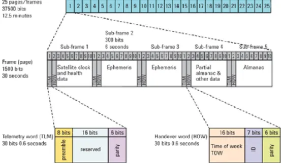
The navigation data have a bit rate of 50 bits per second (bps). The basic format of the navigation data is a 1500-bit-long. This frame has 5 subframes, each having 300 bits.
Figure 2.4 shows the overall structure of an entire navigation message. The navigation message is arranged into thirty bit words. One subframe contains 10 words, each having length of 30 bits. All subframes begin with two special words, the telemetry (TLM) and handover word (HOW). TLM has a fixed preamble of 8-bit pattern 10001011. TLM pattern assists the user equipment in locating the beginning of each subframe. HOW is the truncated version of GPS time of week (TOW). In addition to this HOW contains two flags, one flag indicate the activation of antispoofing, and the other serves as an alert indicator. The alert indicator tells about the accuracy of the signal. If this flag is set then the accuracy might be poor [2].
Figure 2.4 GPS Navigation Message Format[9]
In each frame, the first subframe contains all the clock information and data health indicator. The second and third subframes contain ephemeris data. The last subframes (four
10
and five) alternately provide almanac data and ionospheric correction data. The almanac data is an approximate of ephemeris data for the other satellites in the constellation. It is valid for a longer period of time but its accuracy is less than ephemeris data.
2.4 Trilateration Principle Used in Positioning
GPS is a Time of Arrival (TOA) system which is based on the principle of trilateration.
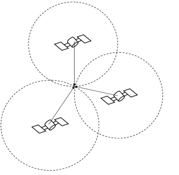
The principle of the trilateration is based on the fact that radio waves propagate at a known speed. Therefore, if we can measure the propagation time of a signal from the transmitter, then the distance between the transmitter and the observer can be measured. If the distances to three transmitters at known locations are given, then the observer can compute its position. The basic idea of trilateration is illustrated in Figure 2.5
11
Three satellites are sufficient for determining the user position but the satellite clocks and the user clocks are not synchronized. Due to this clock bias we need another satellite for the computation of correct position. Since the GPS control segment continuously corrects the satellite clocks and the atomic clocks on satellites are highly stable, the bias is unique to all the satellites. The position of user is calculated with the following Equation (2.5) [2]:
ρs = :8; :<!* =8; =<!* 8; <!* 75< (2.5)
Where ρs denotes the pseudorange between the satellite and the user and x, y, z with subtitles s and r denote the position of the satellites and receivers respectively in Cartesian coordinates. The above model ignores errors caused by ionosphere, troposphere and satellite clock offset. User position can be calculated from the above equation can be solved by iterative numerical techniques or the extended Kalman filter. These methods will be discussed in more detail in Chapter 3 of this thesis.
2.5 Summary
The GPS system is composed of three segments namely: space segment, ground control segment and the user segment. The GPS space segment consists of six orbital planes with at least 4 satellites in each orbit. The GPS ground control segment consists of a master control station and monitoring stations and three ground antennas. The GPS signal consists of sinusoidal carrier wave, PRN sequence and navigation data message. Each satellite has a unique PRN sequence which allows the satellites to broadcast on the same frequency without interfering with each other. The navigation data message enables the user to precisely calculate the position of the satellites.
12
3 Overview
of
Traditional
GPS
Receiver
Architecture
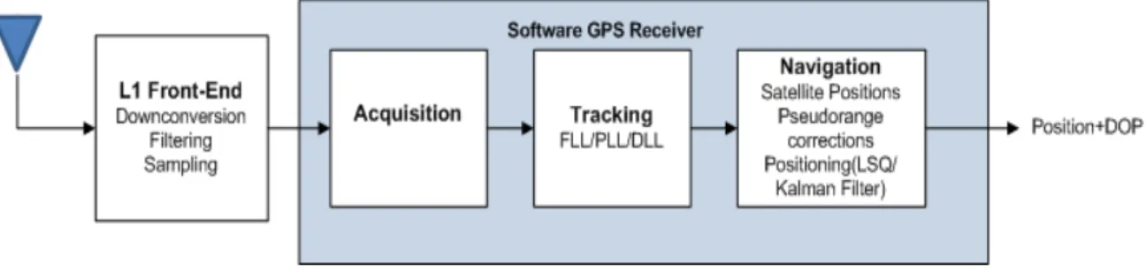
The main functional blocks that constitute a typical GPS receiver are illustrated in the Figure 3.1. In this chapter these functional blocks will be discussed in detail.
Figure 3.1 Generic software GPS receiver
3.1 Antenna
The antenna is the first element in a signal chain of a typical GPS receiver. We will give only a very brief description of the characteristics of a GPS antenna in this section. The signals received from the GPS satellites are very weak and they arrive from virtually any direction and simultaneously from many satellites. The antenna should be able to accommodate the appropriate bandwidth of the desired signal and it should be right-hand circularly polarized (RHCP) as the GPS signals are also RHCP. When the GPS signal is reflected from an object the polarization flips from RHCP to LHCP. An RHCP antenna is quite effective at suppressing the LHCP reflection. Therefore with a RHCP antenna multipath effect can be mitigated. In order to further reduce the multipath error, the antenna pattern of a GNSS receiver is designed in such a way that it receives signals only above 10o-20o elevation, as most of the multipath rays arrive from the low elevation satellites [20].
13
3.2 RF Front End
The first component of a RF front end is a preamplifier. After passing through the preamp stage, the signal is downconverted to an intermediate frequency (IF). The downconverted GPS signal is then filtered and digitized by using an analog to digital converter (ADC).
3.3 Acquisition
The main purpose of acquisition block is to determine which satellites are in view. In addition to this, the acquisition determines the Doppler shift caused by the relative motion of the satellite vehicles and the code phase of the signals. Actually the acquisition stage gives a rough estimate of these parameters and the tracking block further refines them. The acquisition process can be speeded if we have a priori knowledge of the receiver position and satellite almanac. The acquisition stage basically consists of two main phases, carrier-wipe off and code-carrier-wipe off. In the Carrier-carrier-wipe off stage the carrier wave is removed or wiped off by multiplying the incoming signal with a locally generated carrier wave. The GPS signals are affected by the relative motion of the satellites, causing Doppler effect. For a stationary user the Doppler effect can cause a shift of -5 kHz to +5 kHz from the nominal frequency. Therefore the acquisition algorithm should search for different frequencies over this range. Normally a step size of 0.5k Hz is sufficient to search the search the frequency and the same step size has been used in the acquisition algorithm of the software GPS receiver which was used in this thesis. The next stage is code wipeoff in which the incoming PRN sequence is correlated with a local generated C/A code whose code phase has been corrected so that the locally generated C/A code is aligned in time with the received PRN. As mentioned earlier in Chapter 2 the correlation properties of PRN codes are used for determining the satellite PRN number.
Figure 3.2 shows the output of acquisition process. The peak in the Figure 3.2 indicates the highest correlation value. The incoming PRN sequence is multiplied with a locally generated PRN sequence. For each of the different frequencies 1 to1023 code phases are tried. After trying all the possible values, a search for maximum value is performed. If the maximum value exceeds a determined threshold (acquisition metric), the satellite is selected. The frequency at which the peak is located corresponds to the frequency of the carrier wave [20].
14 Figure 3.2 Acquisition [20]
3.4 Tracking
Tracking is the next phase after the successful acquisition of the satellite signals. For the tracking of the satellite signals, a typical GPS receiver deploys code and carrier tracking loops. A phase lock loop (PLL) is used for carrier-phase alignment and a delay lock loop (DLL) is used to maintain the alignment of the code-phase. In the GPS tracking loops, the phase offset of the received and locally generated signal is determined by using the discriminator functions, and each receiver channel tracks the incoming signal independently. This kind of architecture of the tracking loops is called as scalar tracking loop architecture. Tracking loops are a very important part of a GPS receiver as they allow the decoding of the ephemeris data that makes the determination of the satellite position possible. The DLL generates pseudorange measurements which are used in the calculation of the user’s position. Tracking loops will be discussed in more detail in Chapter 4.
3.5 User Position Determination
In order to determine the user’s position data message and pseudorange measurements are used. For the calculation of the user position at least pseudorange measurements from four satellites are required. The pseudorange measurement can be expressed as in Equation (3.7) [12].
15 u
j
j = s −u +ct
ρ (3.1)
Where sj is the number of jth satellite and u is the user. The above equation can be written as a function of user’s coordinates (xu,yu,zu) and the clock bias tu as shown in Equation (3.2) [11]. In this equation the errors caused by the ionosphere, troposphere and the satellite clock offset are ignored.
u u i u i u i j = x −x + y −y + z −z +ct 2 2 2 ) ( ) ( ) ( ρ (3.2)
The user’s position from the above equation can either be determined by using least square solution or using an extended Kalman filter (EKF). Both methods are discussed in detail in the following sections.
3.5.1 Least Square Solution
As mentioned earlier, for calculating the user’s position the Equation (3.4) can be solved by iterative least squares method. We will discuss the least squares solution in detail in this section as in this thesis the least square solution method has been used to obtain the initial positioning solution followed by an EKF. In least squares solution, nominal estimation of the user’s position and the clock bias is chosen first. Then the pseudorange formulas are Taylor linearized about the nominal value. The resulting linear system of equations produces corrections in the user’s position and clock bias. These corrections are then added to the initial estimates. The corrected estimates are then used to linearize the pseudorange equation. Corrections are calculated again to obtain further refined estimates. This iterative process continues until the estimated values approach the constant values. Before using the Equation (3.4) in least square solution, the pseudorange equation should be linearized. The main steps in the linearization are elaborated in the next section. Complete linearization details can be found from [2].
16 3.5.2 Linearization of Pseudorange Equations
Pseudorange measured to the ith satellite as in Equation (3.2) can also be expressed in the form of Equation (3.3). ) , , , ( u u u u i = f x y z ct
ρ
(3.3)True user position and clock bias are:
u u u u u u u u u u u u t c t c t c z z z y y y x x x δ δ δ = + ∆ ∆ + = ∆ + = ∆ + = ˆ ˆ ˆ ˆ
Based on these relations the equation can be rewritten as a function of nominal trajectory plus the error terms as expressed in the Equation (3.5).
) ˆ , ˆ , ˆ , ˆ ( ) , , , (xu yu zu ctu f xu xu yu yu zu zu c tu c tu f = +∆ +∆ +∆
δ
+∆δ
(3.4) From this point the pseudorange equations can be linearized by expanding the equations using Taylor series. The Taylor series is truncated at the first order; therefore the function determines an approximate position. By using the partial derivatives obtained from the 1st order Taylor series expansion we get Equation (3.5).u u i u i u i u i u i u i i i i z c t r z z y r y y x r x x δ ρ ρ ρ = − ≈ − ∆ − − ∆ − − ∆ +∆ ∆ ˆ ˆ ˆ ˆ ˆ ˆ ˆ (3.5) 2 2 2 , , , , ) ˆ ( ) ˆ ( ) ˆ ( ˆ j u j u j u u u i z i y u i y u i x i z z y y x x r t c z a a y a x a where − + − + − = ∆ − ∆ + ∆ + ∆ = ∆
ρ
δ
(3.6)The linearized pseudorange equations can be written in the form of concise matrix formulation as shown in the Equation (3.7)
17 ∆ ∆ i ρ ρ M 1 ∆ ∆ ∆ ∆ − − ≈ u u u u i z i y i x z y x t z y x a a a a a a 1 1 , , , 1 , 1 , 1 , M M M M (3.7) x H∆ = ∆
ρ
(3.8)There can be three different possibilities at this point. First possibility could be that if there are less than four pseudorange measurements, then this system of equations cannot be solved. If we have four pseudorange measurements then we solve this system of equations by inverting the matrixH [2].
ρ
∆ = ∆ −1 H x (3.9)When more than four pseudorange measurements are available then the inverse will not be unique anymore and the inverse is called as pseudoinverse. Such system of equations is then solved using Moore-Penrose pseudoinverse as shown in the Equation (3.10) [2]
ρ
∆ = ∆ T − T H H H x ( ) 1 (3.10)Where HTis the transpose of the matrix H.
The vector of corrections is added to the approximate receiver position to get next refined estimates of the user’s positions and clock correction. These new estimates are then used to produce more accurate estimates by repeating the process until ∆xi,1,∆yi,1,∆zi,1 are at meter level.
3.5.3 Extended Kalman Filter
The least squares solution is a point solution and user’s states like clock and platform dynamics cannot be modeled in this kind of solution. On the other hand extended Kalman filter (EKF) is a recursive algorithm and it can incorporate the knowledge of the previous measurements into current estimates and more refined results can be obtained [17]. And not only its recursive nature makes it more suitable for GPS applications but user’s clock and dynamics can also be modeled in this algorithm.
In this thesis an EKF for stationary user has been implemented so EKF model for stationary user scenario will be discussed in this section. The EKF in GPS tracks the errors in the user’s states and not the actual user’s states. The user’s states are kept outside of the filter and at each measurement epoch the estimates of errors are added in the user’s states and the vector containing the errors in the user’s states in reset to zero. Pseudoranges are used as measurements in the EKF and at each iteration the estimates are used to linearize the pseudorange equations.
18
The states
δ
x, δyandδ
zcorrespond to errors in the estimated x, y and z coordinates of the user in the Earth Centered-Earth Fixed (ECEF) reference frame. The statesδ
t andδ
t& are the errors in the clock bias and clock drift respectively.[
]
T k k k k k y z t t xδ
δ
δ
δ
&δ
(3.11)The state transition matrix ‘ø’ is given as in Equation (3.12).
∆ = 1 0 0 0 0 0 0 0 0 0 0 1 0 0 0 0 0 1 0 0 0 0 0 1 T
φ
(3.12)In the above matrix ∆T is the filter update rate.
The estimates of the user states are used to linearize the observation matrix as shown in the Equation (3.13). = 0 1 0 1 , , , 1 , 1 , 1 , i z i y i x z y x a a a a a a H M M M M M (3.13)
In the measurement matrix H which is also called as geometry matrixax,i, ax,i and ax,i are the components of a unit vector pointing from the user’s estimated position to the ith satellite.
Pseudoranges are used as measurement for the EKF; their model equation is given in Equation (3.14). u i i i i u i i (x xˆ ) (y yˆ ) (z zˆ ) ctˆ ˆ = − 2 + − 2 + − 2 + ρ (3.14)
The measurements used by the filter are range residuals which arre the difference between the predicted pseudoranges and the observed pseudoranges. The measurement update step consits of multipication of the measurement vector and the kalman gain. The estimated error state vevtor is then added to the estimates of the user’s states outside the filter. The updated user state vector is projected ahead for the next measurement epoch and the error state vector is reset.
The process noise covariance matrix is denoted by ‘Q’ and it is a diagonal matrix with zeros off the principal diagonal. The diagonal elements of the process noise covariance matrix are used to model the velocity and clock variances. In this thesis process noise covariance matrix has been selected as identity matrix.
19
The measurement noise covariance matrix ’R’ is given in the Equation (3.15) which is a diagonal matrix [2]. The diagonal elements of the measurement covariance matrix depend on the vairance on pseudornage measurement.
=
2 2 10
0
0
0
nR
ρ ρσ
σ
L
M
O
M
L
(3.15)20
4 Scalar Tracking Loop Design
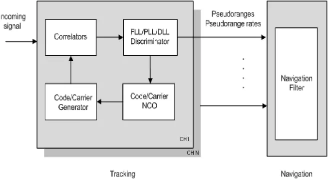
In this chapter the scalar tracking loop architecture that is deployed in the traditional GPS receiver is explained in detail. As mentioned earlier also the tracking loop that are implemented in a typical GPS receiver are also called as scalar tracking loops as each receiver channel processes the received signal individually
Figure 4.1 Scalar tracking loop architecture
Figure 4.1 shows a graphical representation of a generic GPS receiver. There the loops are close inside each channel (CHn), and only pseudoranges or pseudorange rates are fed forward to the navigation processor. The scalar tracking loops operate well under better
/>! ratio and low user dynamics. However they do not give optimal performance in
weak signal environment. This is due to the fact that tracking loops track every satellite signal independently so lock on one satellite does not help to track the other satellite. This type of architecture has relatively easier implementation and is robust in the sense that error in one channel cannot corrupt the other channel. However aiding of the weaker signals is not possible by the presence of relatively stronger satellite signals and the inherent relation between the signals and the user states is completely ignored.
21
The scalar tracking loops use fixed bandwidth filters that are unable to adapt to the varying
/> levels and user dynamics. The measurements made by the discriminators during
periods of low /> are weighted equally to the measurements made in the high /> level.
4.1
Carrier Tracking
A carrier tracking loop is necessary to remove the carrier frequency modulation from the incoming signal, therefore the incoming carrier signal’s frequency and phase must be accurately replicated. The carrier tracking loop is always the weakest link in a standalone GPS receiver, its threshold characterizes the performance of an unaided GPS receiver [2]. Therefore careful designing of carrier tracking loops is needed. A carrier tracking loop can be implemented as a Costas loop, phase lock loop (PLL) or frequency lock loop (FLL) or a combination of both PLL and FLL depending upon the nature of the application.
4.1.1 Phase Lock Loop
For the demodulation of the navigation data an exact replica of the carrier wave has to be generated a phase lock loop (PLL) is usually used in a GPS receiver. A PLL is sensitive to 180° phase shift, and for a GPS receiver it is very important that the PLL should be insensitive to the 180° phase shift that occur due the navigation data bit transitions. On the other hand a Costas loop is insensitive to this phase reversal. Therefore a PLL is typically implemented as Costas loop in a GPS receiver. The disadvantage of using the Costas loop is that there is a 6 dB tracking-sensitivity as compared to a Pull-Phase Locked Loop (P-PLL) [14]. Therefore in a GPS receiver the PLL is more sensitive to environment noise, interference and jamming and it loses the lock first. The Costas loop contains two multiplication operations. The received carrier plus data signal is fed into the loop. The input is then multiplied by the loop's in-phase (I) estimate of the carrier in the upper arm and in the lower quadrature (Q) arm the signal is multiplied by a 90° phase shifted carrier wave.
22 Figure 4.2 Phase lock loop
23
PLL Discriminator
A two-quadrant arctangent non-linear discriminator function is used in PLL which has optimal performance for high and low SNR. The output of this discriminator is phase error. Some of the other possible discriminators are described in [2].
) ( tan 1 I Q D= − ( 4.1)
In a software GPS receiver the low pass filters in the both arms of the Costas loop and the other tracking loops are replaced by 'integrate and dump' functions which are nothing but integrators. This change is necessary due to the fact that signals in a software receiver are sampled instead of being continuous. The products in the I and Q channels are summed over an integration interval. The integration period is coordinated in such a way that it does not integrate over data but transition. After passing through the discriminator the output is fed to the numerically controlled oscillator to close the feedback loop.
4.1.2 Frequency Lock Loop
Frequency lock loop (FLL) is also called as automatic frequency control (AFC) loops as they perform the carrier wipeoff process by replicating the approximate frequency. FLL is normally used for the initial lock purpose in a GPS receiver [2]. This is because during the initial stage of acquisition the receiver normally does not know where the data transition boundaries are and the FLL discriminators are less sensitive to situations where some of the I and Q signals do straddle the data bit transitions. FLL has a lower tracking threshold as compared to a PLL. Therefore FLL has the ability to keep lock on the incoming signal after the PLL has lost lock. This kind of situation typically exists in GPS challenged environment where the signal power is very low. The method of decoding the navigation data bit directly from a FLL has been discussed in [15].
FLL Discriminator
The FLL discriminators calculate the frequency error by collecting integrated and dumped prompt samples IPS1 and QPS1 at time t1 and integrated and dumped prompt samples IPS2 and
QPS2 at a later time t2.The adjacent sample time interval (t2-t1) cannot straddle a data bit
transition. The accuracy of the carrier frequency is a few hundred Hertz after the acquisition stage. In order to bridge the acquisition and FLL the carrier frequency is tracked in two stages by using two different discriminator algorithms [15]. Initially a coarse tracking discriminator is deployed, e.g. four quadrant frequency discriminator given in Equation (3.2) [2].
24 # ?@?2ABCDD, EC !
; ! 360
(4.2) The four-quadrant arctangent discriminator function has optimal performance at both high and low SNR. But it has the highest computational burden also. Then a cross-product discriminator given in Equation (3.3) [2] is used for fine carrier tracking which is followed by a low-pass loop lifter to remove high frequency portion of the incoming signal.
D signdot!crosst ; t (4.3) where: dot IOP . IOQ* QOP . QOQ (4.4) cross IOP . QOQ; IOQ. QOQ (4.5)
4.2 Code Tracking
The code tracking loop keeps track of the code phase of a specific code in the signal. An ideal code tracking loop generates a code signal that is a perfect replica of the incoming signal code. In a GPS receiver code tracking loop is implemented as a delay lock loop (DLL).
4.2.1 Delay Lock Loop
The DLL operates by generating three replicas of the received code. These replicas are called as early, prompt and late of the code. The incoming signal is converted to baseband, by multiplying it with a perfectly aligned local replica of the carrier wave. Later on the signal is multiplied with three code replicas. The output signals are then integrated and dumped. The result is a numerical value which indicates how much the specific code replica correlates with the incoming signal. The replicas are nominally generated by ±½ chip. The three correlation outputs are then compared to see which one provides the highest correlation.
25 Figure 4.3 Delay lock loop [20]
DLL Discriminator
The DLL discriminators can be broadly divided into two categories: Coherent and non-coherent discriminators. The non-coherent discriminators require phase lock (PLL tracking). All power is in the in-phase of signal. Coherent discriminators are used in simple receivers in order to reduce the number of correlators. On the other hand the non-coherent discriminators are not dependent on PLL as they use the both in-phase and quadrature arms. Both types of the discriminators have been enlisted in [2].
S TUV1 * WV1 X ; U1 * W1 ! TUV1 * W V1 X * U 1 * W 1 ! (4.6)
In a GPS receiver normally a normalized early minus late power discriminator is used as it is independent of the performance of the PLL. The signals power in urban canyons and in indoor environment changes rapidly due to receiver motion. Therefore the discriminator is normalized so that the discriminator can be used with signals with different signal-to-noise ratios and different signal strengths and it is independent of signal's amplitude. Another important factor for choosing the normalized early minus late power discriminator is that it has the highest processing gain and its gain increases when the correlator spacing decreases [16]. In order to suppress the DLL tracking error caused by multipath use of narrow correlators spacing has been proposed [2]. Therefore taking account of all these factors normalized early minus late power discriminator seems the obvious choice. For this thesis correlator spacing of ½ chip has been used.
26
4.3 PLL aided DLL
Combining both PLL and DDL can also reduce the multiplication operations in the PLL which speeds up the computation time. In addition to this the PLL-aided DLL design reduces the dynamics of DLL significantly to 0.1 Hz [2].
Figure 4.4 Combined code and carrier tracking loops [20]
27
4.4 Parameters effecting tracking loop performance
In this section parameters that affect the performance of the tracking loops are briefly discussed. Following parameters are very important in the characterization of the tracking loops in GPS receiver.
4.4.1 Loop discriminators
The tracking loop discriminators are characterized by their normalization requirements, as this may be significant in low signal power cases. In addition they are characterized by their computational burden and their response under Gaussian noise [2].
4.4.2 Loop filter
The loop filters are used in the tracking loops to reduce the noise in order to produce an accurate estimate of tracking error. The performance of the loop filter is determined by its order and allowed noise bandwidth. Both of these factors determine the response of the filter to the signal dynamics [2].
The first order filter is sensitive to velocity stress, second order is sensitive to acceleration stress and third order is sensitive to jerk stress. For phase tracking loop, a third order filter is normally used in order to track the user dynamics. For code tracking loop first order loop is usually enough as it is aided by carrier tracking loop and most of the dynamics are already removed in carrier tracking loop. Therefore the code tracking loop estimates only code errors due to ionospheric divergence.
The loop filter bandwidth defines the level of noise allowed in the tracking loop. If the noise bandwidth is decreased the estimated errors are decreased. The noise bandwidth can be increased for robustness to dynamic stress. In the third order loop the noise bandwidth can be increased to 18 Hz, which makes it suitable for high dynamics situation [2].
4.4.3 Predetection integration time
Predetection integration time is a very important parameter in tracking loops. The predetection integration time determines the update rate of the loop. If we increase the predetection time we can gather more power of signal but it is always highly possible that the signals dynamics might be changing during the integration period. The predetection integration in L1 signal is limited to 20ms which is the duration of data bits [2].
28
5 Vector Tracking Loop Design
In this chapter, the vector tracking loop based modern GPS receiver architecture is introduced and its potential benefits over scalar tracking loops are explained. Later in the chapter, a Vector Delay Lock Loop which has been implemented in this thesis is explained in detail.
5.1 Vector Tracking Loop Architecture
In vector tracking loops the signal processing is done in an aggregate manner Therefore mutual aiding of the weaker satellite signals can be achieved by the presence of stronger satellite signals [18]. The very first approach of vector tracking was presented as a Vector Delay Lock Loop (VDLL) which proposed combining the task of the signal tracking in the navigation filter was presented in [3]. It was shown in [3] that user’s position can be determined by using the information from the stronger satellite signals and the weak signals in turn can then predicted on the basis of the states of the user [3]. The tracking and navigation are not independent anymore as compared to the traditional receiver architecture and all of the tracking channels are combined via EKF. This architecture can track the temporarily attenuated or blocked signals because the navigation results can still be derived from the other visible satellites.
29 Figure 5.1 Vector tracking loop proposed by Spilker
30
5.2 Vector Tracking Loop Architecture based on Discriminator
The architecture of the VDLL can be different depending on its implementation. Various variants of VDLL have been implemented in [4] [5] [6] [7]. VDLL based on discriminator function was presented in [4] and its performance was analyzed by the simulated data. In a discriminator based VDLL, the tracking input is not directly connected to the tracking control input rather the discriminator output is used in estimating pseudoranges. The EKF in turn predicts the code phases. In VDLL all channels are processed together in one processor which is typically an extended Kalman filter (EKF). Therefore, even if the signals from some satellites are very weak the receiver can track them from the navigation results of the other satellite. VDLL is a very attractive technique as it can provide tracking in very weak signal environment. Moreover the size of the VDLL based GNSS receiver is very small as compared to an augmented GNSS receiver and power cost is also lower as it does not need any external hardware. The interference benefits of the VDLL were studied in [5]. Another variant of VDLL augmented with inertial navigation system (INS) was presented [6]. The VDLL based receiver is illustrated in Figure 5.2. From the figure we can see that the output of the VDLL is directly passed to the navigation filter and is used in position estimation. The EKF in turn controls the code NCO. A Vector delay lock loop based on the discriminator output has been implemented in this thesis and it will be discussed in detail later in this chapter.
31 Figure 5.2 Vector tracking loop based on discriminator
5.3 Vector Tracking Loops Based on Adaptive Estimation
Method
Despite of the several benefits that can be achieved from the vector based receiver, the vector tracking loop design has some inherent flaws which make them less robust for high dynamic situations. For example, if the error in one channel becomes large, it is propagated to all the channels through the navigation filter. On the contrary, the scalar tracking loops the channels are isolated from each other so error in one channel doesn’t affect other channels. Under high dynamic situations the navigation filter may not track the states as the Doppler frequency changes faster with time. Therefore, Doppler estimation becomes the limiting factor for the performance of the vector tracking loops [19].
In order to cope with this situation, an adaptive estimation method for tracking the change in the Doppler frequency has been presented in [19]. This technique, illustrated in Figure 5.3 uses vector tracking loop based on discriminators of DLL, FLL and PLL. It employs an adaptive two-stage Kalman filter which is capable of adapting to the quickly changing Doppler frequency. With this method the minimum threshold of /> of 35dB-Hz can be achieved [19].
32 Figure 5.3 Vector tracking loop based on adaptive estimation method
5.4 Vector Delay Lock Loop Based on Discriminator
This section describes the VDLL that has been implemented in this study. For the implementation of a VDLL we need only four states of the user i.e. user position coordinates and clock bias. Therefore clock drift can be omitted from the state transition model which was illustrated in Chapter 3. This is how performance gain is achieved in VDLL as n pseudorange residuals are used to determine four user states. On the other hand conventional GPS receivers use n scalar DLLs to determine n pseudoranges. The user states are related to range residuals in VDLL as shown in Equation (5.1)
=
t
c
z
y
x
a
a
a
a
a
a
n z n y n x z y x nδ
δ
δ
δ
ρ
δ
ρ
δ
1
1
~
~
, , , 1 , 1 , 1 , 1M
M
M
M
M
(5.1)The measurement noise covariance matrix in VDLL is a diagonal matrix and its diagonal elements are the variances of the early minus late discriminator which has been used in the algorithm.
33
=
2 , 2 1 ,0
0
0
0
nR
δτ δτσ
σ
L
M
O
M
L
(5.2)The VDLL developed in this thesis is based on the discriminator function. It uses a normalized early-minus-late discriminator to estimate the code phase error. This discriminator uses the output of the early and late correlators.
Y
TZ[\] ^_[\] X`Za\] ^_a\] ! TZ[\] ^_[\] X^Za\] ^_a\] !( 5.3)
where: Y is the discriminator output in chips;
IES and QES are inphase and quadraphase components of early (E) and ILS and QLS are
inphase and quadraphase components of late (L) correlators.
Figure 5.4 shows an overview of the vector tracking loop architecture used in this thesis. The receiver initially operates in the scalar mode with scalar DLL and PLL until at least four satellites are acquired and sufficient accurate positioning solution is obtained. For the purpose of obtaining the initial solution, the least squares solution has been used in the implementation of the VDLL algorithm in this thesis. After that the receiver operates in the vector tracking mode.The VDLL implementation algorithm in this thesis is based on the technique presented in [7].
Figure 5.4 Overview of the VDLL technique
The discriminator output is modeled as the difference between the true pseudorange
ρ
true and the measured pseudorangeρ~ .34
n
true
−
+
=
∆
ρ
~
ρ
ρ
~
( 5.4)where: n is the pseudorange estimation noise which is linearized.
The VDLL algorithm starts with the discriminator output ∆ρ~ and the pseudorange measurement ρ~ . Instead of the observed or the measured pseudorange estimated pseudorange
ρ
ˆ is used for the reference value for the C/A code to be generated. The residuals ofρ
ˆare zero by definition. An error estimate (ρ
~+∆ρ
~)−ρ
ˆ is used as an input to the EKF. The construction of the EKF is shown in Figure 5.5 [17].Figure 5.5 Extended Kalman filter in VDLL [17]
The reference pseudorange is estimated from the Equation (5.5) which is updated from the EKF navigation results.
u u i u i u i x y y y y ct x ) ( ) ( ) . ( ˆ = − 2 + − 2 + − 2 + ρ (5.5)
where: xi,yi,zi and xu,yu,zuare the
x
,
y
,
z
position of the ith satellite and user estimated position and tu is clock bias respectively.The estimates of the pseudorange error ∆
ρ
ˆ are calculated by multiplying the innovation term of the EKF ∆xˆwith the Jacobian matrix H which contains the user satellite geometry.x H. ˆ
ˆ = ∆
35
The reference pseudorange is calculated by adding the updated pseudorange estimate and the pseudorange error estimate as shown in the Equation (5.7).
ρ
ρ
ρ
ˆ+ = ˆ +∆ˆ (5.7)The tracking control input is the difference between the measured pseudorange ρ~ and the reference pseudorange
ρ
ˆ +ρ
ρ
ρ
ˆ = ˆ − ~ ∆ + + (5.8) Figure 5.6 Illustration of VDLL5.5 Summary
In this chapter vector tracking loop method was presented and its benefits over scalar tracking loops were explained. The shortcomings in the vector tracking approach were also very briefly explained and one of the proposed solutions was also presented. Later in the Chapter implementation detail of the Vector Delay Lock Loop algorithm was presented, which combines the tracking of the PRN code phases and estimating the user’s position together. The VDLL implemented in this thesis is based on the discriminator function. An
36
early minus late discriminator is used in this thesis and the control input to the tracking loops is generated by subtracting the reference pseudorange from the measured pseudorange. The VDLL has the ability to perform in degraded signal environment and can significantly bridge momentarily signal outages. In the following chapter simulation results will be presented and it will be shown that VDLL can operate at lower /> ratio and during the satellite outage period.
37
6 Simulation Results
In this chapter the benefits of the VDLL introduced in the Chapter 5 during momentary blockage are investigated. In addition to this the ability of VDLL to operate at nominal
/ levels is also verified. The simulation results prove the ability of VDLL during the
satellite outage period and low / ratio.
6.1
Simulation Setup
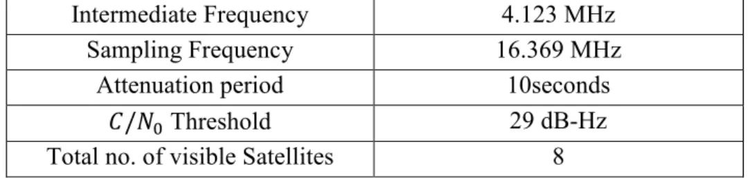
The VDLL algorithm discussed in Chapter 5 was implemented in MATLAB environment. An existing, open source software receiver [20] was used as the base of the VDLL developed in this study. In order to study the behavior of the VDLL, simulated data was used which was generated from the Spirent STR 4500 simulator [8] for a stationary receiver. The GPS signals were down-converted, sampled and saved by a commercial GPS radio frequency front end at an intermediate frequency of 4.123 MHz and sampling frequency of 16.369 MHz [21]. Eight GPS satellites (numbers 1, 7, 8, 10, 13, 15, 20 and 22) were visible.
38
At approximately 50 seconds after the start of the simulation, the power of the signal from satellite 10 was attenuated rapidly for about 10 seconds, which caused momentary blockage and after that the signal returned to its previous level. The update rate of the measurements and propagation for the EKF was set to 20ms. For comparison purpose standard DLL was used for the tracking of PRN code. The DLL used a normalized early minus late discriminator and a noise bandwidth of 2 Hz. For both VDLL and DLL an integration time of 20ms was used.
Intermediate Frequency 4.123 MHz Sampling Frequency 16.369 MHz
Attenuation period 10seconds
/ Threshold 29 dB-Hz Total no. of visible Satellites 8
Table 6.1 Simulation setup parameters
6.2 Code Tracking Results of Scalar DLL
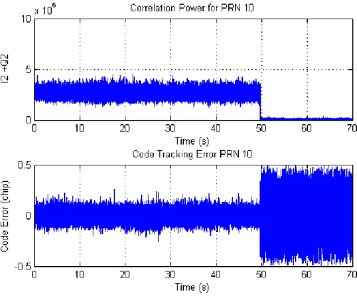
Figure 6.2 shows the tracked signal power of PRN 10 which is obtained by correlation magnitude ∑ I2 +Q2 of the in-phase prompt and quadrature-phase prompt accumulation values. Figure 4 shows the behavior of scalar tracking loop. From the Figure 6.2, we can see that when the signal power from the satellite number 10 is rapidly decreased, a momentary blockage of the signal is caused and the correlation power amplitude virtually drops to zero. The code discriminator only produces accurate estimates of the phase error when the codes are aligned to within a range of half a chip. Outside of this range the discriminator output is dominated by noise. The code phase estimates of the scalar DLL diverge during the attenuation period. When the attenuation period is over the code phase estimates are not within the half a chip of the true code phase. Therefore the scalar DLL fails to reacquire the signal when the signal reappears after 10 seconds.
39 Figure 6.2 Code tracking results of scalar DLL
6.3
Code Tracking Results of Vector Delay Lock Loop
Figure 6.3 show the code tracking results obtained from VDLL. When the /> falls below the threshold the diagonal terms of the measurement noise covariance matrix are inflated and the VDLL algorithm starts ignoring the measurements. We can see that during the signal attenuation period the VDLL ignores the code phase measurements from the PRN 10 and it uses its own estimates of code phase error. The output of code discriminator is dominated by noise during the attenuation period and after the signal returns the code discriminator shows valuable output. Therefore it can be concluded that the algorithm’s code phase estimates are sufficiently accurate so that the code discriminator produces accurate estimates as soon as the signal returns to its previous /> level. It can also be seen that the VDLL recovers the correlation power instantly ascompared to scalar DLL. The variance of the output of the code phase discriminator is reset to its original value after the blockage period is over.
40 Figure 6.3 Code tracking results of VDLL
6.4 Navigation Results
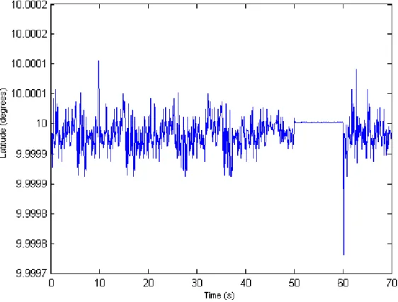
In order to investigate that whether the VDLL can provide navigation solution when less than 4 satellites are in view, another data set was simulated. The main parameters of the data set are the same as mentioned in Table 6.1. At approximately 50 s in the simulation power of 6 satellites is attenuated to 29 dB-Hz. Therefore only 2 satellites are available for the calculation of the navigation solution. The user is stationary and is located at North latitude of 10o, 0’, East longitude of 10o, 0’ and an altitude of 0 meters. Iterative least squares method is used to get the first position fix and after that EKF is used for estimating the user’s position.
From the Figure 6.5, Figure 6.5 and Figure 6.6 it can be seen that VDLL is able to provide navigation solution which proves VDLL’s superior performance over scalar tracking method. The results are plotted in East, North and UP (ENU) coordinates. In these figures we can see that during the satellites attenuation period the user’s position estimates remain almost static. This is because that during the attenuation period the diagonal elements of the measurement covariance matrix are inflated and the EKF starts ignoring the
41
measurements. When the satellites return to its previous power level and the EKF starts to estimate the user’s position based on the code discriminator output.
42 Figure 6.5 User’s longitude estimate
43 Figure 6.6. User’s altitude estimate
From the Figure 6.6 we can see that the estimate of the user’s altitude is negative and as the simulation proceeds the estimate of user’s altitude is converging to the correct value. The negative altitude is mainly due to the fact that GPS receiver obtains an altitude value comparative to sea level but not to ground level
44
7 Conclusion and Future Work
In this thesis a receiver architecture based on the vector tracking loops was presented. In this type of receiver architecture, the vector tracking algorithm combines the operation of tracking and navigation state estimation in a single algorithm. The benefits of the vector tracking loops were presented and their flaws were also discussed. Out of the various advantages of vector tracking loops that have been presented we investigated the ability of the vector tracking loops to operate at significantly lower / level and the bridge the momentarily signal outage. For this purpose we replaced the scalar DLL with vector delay lock loop. The vector delay lock implemented in this thesis is based on the discriminator function which uses nonlinear discriminator function and an extended Kalman filter to track the PRN code phase. The performance of the VDLL was compared with scalar DLL by using simulated GPS data. The simulation results clearly showed the superior performance of VDLL over traditional DLL. VDLL algorithm developed in this thesis outperformed the scalar DLL during the temporary satellite outage period. From the simulation results it was shown that VDLL was able to recover correlation power of the signal after the attenuation period whereas scalar DLL was unable to recover the correlation power of the signal. Therefore the VDLL has the potential to operate in degraded signal environment where the traditional methods fail.
There is a great room for future work in the algorithm presented in this thesis. First of all there is great need of developing appropriate channel ca
![Figure 4.4 Combined code and carrier tracking loops [20]](https://thumb-us.123doks.com/thumbv2/123dok_us/468771.2555275/34.918.196.755.296.820/figure-combined-code-carrier-tracking-loops.webp)

![Figure 5.5 Extended Kalman filter in VDLL [17]](https://thumb-us.123doks.com/thumbv2/123dok_us/468771.2555275/42.918.259.772.344.765/figure-extended-kalman-filter-in-vdll.webp)