E
NERGY AND
E
NVIRONMENT
Volume 3, Issue 4, 2012 pp.617-628
Journal homepage: www.IJEE.IEEFoundation.org
Effect of flow field on open channel flow properties using
numerical investigation and experimental comparison
I. Khazaee
1, M. Mohammadiun
21 Department of Mechanical Engineering, Torbat-e- jam branch, Islamic Azad University, Torbat-e- jam, Iran.
2 Department of Mechanical Engineering, Shahrood branch, Islamic Azad University, Shahrood, Iran.
Abstract
In this paper a complete three-dimensional and two phase CFD model for flow distribution in an open channel investigated. The finite volume method (FVM) with a dynamic Sub grid-scale was carried out for seven cases of different aspect ratios, different inclination angles or slopes and convergence-divergence condition. The volume of fluid (VOF) method was used to allow the free-surface to deform freely with the underlying turbulence. The discharge through open channel flow is often evaluated by velocity-area integration method from the measurement of velocity at discrete locations in the measuring section. The variation of velocity along horizontal and vertical directions is thus very important to decide the location of the sensors. The aspect ratio of the channel, slope of the channel and divergence- convergence of the channel have investigated and the results show that the depth of water at the end of the channel is higher at AR=0.8 against the AR=0.4 and AR=1.2. Also it is clear that by increasing the inclination angle or slope of the channel in case1, case4 and case5 the depth of the water increases. Also it is clear that the outlet mass flow rate is at a minimum value at a range of inclination angle of the channel.
Copyright © 2012 International Energy and Environment Foundation - All rights reserved.
Keywords: VOF model; Channel aspect ratio; Open channel; Velocity distribution.
1. Introduction
Open channel flows are found in Nature as well as in man-made structures. In Nature, tranquil flows are observed in large rivers near their estuaries: e.g. the Nile River between Alexandria and Cairo, the Brisbane River in Brisbane. Rushing waters are encountered in mountain rivers, river rapids and torrents. Classical examples include the cataracts of the Nile River, the Zambesi rapids in Africa and the Rhine waterfalls[1].
In contrast to empirical studies, numerical investigations of open channels are limited because it is much more difficult to model flow in open channels than in closed conduits. This is because flow conditions in open channels are complicated by the fact that the position of the free surface is likely to change with respect to time and space. Recently Direct Numerical Simulation (DNS) for open channel flows have been reported, but most of these simulations assume (1) that the free surface is a rigid slip surface and its vertical movement is neglected, as was the case in Nagaosa [2], or (2) simply apply the linearized free-surface boundary conditions, as in the case of Borue et al. [3].
Mathematical models of the velocity profile in circular pipes are available [4] and have been used for determining the most appropriate locations of current meters/acoustic transducers for minimizing the systematic error in discharge measurement in circular penstocks. However, to the best of authors’ knowledge, such mathematical models are not available for open channels. In the open channel flow, the velocity distribution along the vertical direction (depth) is theoretically represented by a logarithmic function of the depth of flow [5]. It is very difficult to describe the velocity distribution along the width theoretically. However, some of the investigators have proposed empirical equations for the velocity distribution based on experimental and field data [6-9].
In this work a three-dimensional and two phase CFD model for an open channel flow has investigated to study the flow distribution for different open channels with different aspect ratios and convergence- divergence geometries. This CFD model developed for a real open-channel was first validated by comparing the velocity profile obtained from it with that obtained by actual measurement in the same channel. All the geometries are modeled with similar operating and boundary conditions. Fluent 6.3.26®, a finite volume computational fluid dynamics package, was used to solve the non-linear system of equations.
2. Numerical model
The three dimensional equations together with the continuity are solved using the finite volume method with implicit formulation and first order discrete method that the relation of the pressure and velocity is with the simple algorithm. Transport equations for turbulence kinetic energy k and its dissipation ε are solved for “closing” the system of equations. In addition a modified volume of Fluid (VOF) method was employed for computing the free surface.
The model was implemented into the commercial CFD code FLUENT 6.3.26 with custom developed user-define functions (UDF)
The VOF formulation relies on the fact that two or more fluids are not interpenetrating. For each additional phase a variable is introduced, the volume fraction of the phase in the computational cell. In each control volume, the volume fractions of all phases sum to unity. The fields for all variables and properties are shared by the faces and represent volume averaged values. Thus the variables and properties in any given cell are either representative of one of the faces, or representative of a mixture of the faces, depending upon the volume fraction values. The flow involves existence of a free surface between the flowing fluid and the atmospheric air above it. The flow is generally governed by the forces of gravity and inertia. In VOF model, a single set of momentum equations is solved for two or more immiscible fluids by tracking the volume fraction of each of the fluids throughout the domain. The mathematical formulation adopted is described briefly below.
In the current study, it is assumed that the density of water is constant through the computational domain. The governing differential equations of mass and momentum balance for unsteady free surface flow can be expressed as:
0
)
.(
=
∇
+
∂
∂
u
t
G
ρ
ρ
(1)g
u
p
u
u
t
u
G
G
G
G
G
+
∇
∇
+
∇
−
=
∇
+
∂
∂
)
.(
1
)
.(
ν
ρ
(2)where uG is the velocity vector in the three directions; P is the pressure; ν is the molecular viscosity;
g
G
is the gravitational acceleration in the three directions, and ρ is the density of flow.Small high-frequency fluctuations are present even in steady flow and, to account for these, time averaging procedure is employed, which results in additional terms. These additional terms need to be expressed as calculable quantities for closure solutions. The standard κ-ε model has been used in the present case. It is a semi-empirical model based on model transport equations for the turbulent-kinetic energy ‘κ’ and its dissipation rate ‘ε’, and is expressed by the following equations:
ε
ν
σ
ν
−
⎟
⎟
⎠
⎞
⎜
⎜
⎝
⎛
∂
∂
+
∂
∂
∂
∂
+
⎟
⎟
⎠
⎞
⎜
⎜
⎝
⎛
∂
∂
∂
∂
=
∂
∂
+
∂
∂
j i i j j j T j k T j j jx
u
x
u
x
u
x
k
x
x
k
u
t
k
(3) 2ε
ν
T=
c
µk
(4)The dissipation of k is denoted ε, and modeled as:
k
C
x
u
x
u
x
u
k
C
x
x
x
u
t
j i i j j j T j T j j j 2 2 1ε
ν
ε
ε
σ
ν
ε
ε
ε ε ε+
⎟
⎟
⎠
⎞
⎜
⎜
⎝
⎛
∂
∂
+
∂
∂
∂
∂
+
⎟
⎟
⎠
⎞
⎜
⎜
⎝
⎛
∂
∂
∂
∂
=
∂
∂
+
∂
∂
(5)The constants in the k-ε model have the following values:
c
µ=0.09,C
ε1=1.44,C
ε2=1.92,σ
k=1.0 and εσ
=1.30.The properties appearing in the transport equations are determined by the presence of the component phases in each control volume. For a N-phase system, the volume fraction-averaged density takes the following form:
∑
=
q qρ
α
ρ
(6)For “tracking” the free surface the continuity equation for the volume fraction is used. For the qth phase, this equation has the following form:
0
=
∂
∂
+
∂
∂
i q i qx
u
t
α
α
(7) The volume fraction equation is solved for each phase except the one that is defined as primary. For the primary phase the volume fraction is computed based on the following constraint:∑
= = n q q 1 1α
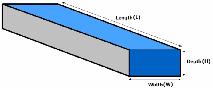
(8)The physical problem considered in this paper is the three dimensional model of the open channel as shown in Figure 1 that the dimensionless parameter in this paper named aspect ratio,
H W
AR= ,is
defined to characterize the geometric effect of the channels. In Table 1 the characteristics of the channels such as depth, width, length and slope are shown.
Figure 1. The simulation domain Table 1. Detail of the different cases
Case H(cm) W(cm) L(cm) Slope(deg) 1 12.6 15.2 60 0.057 2 12.6 10.08 60 0.057 3 12.6 5.04 60 0.057 4 12.6 10.08 60 0.1145 5 12.6 10.08 60 0.573 6 (convergence) 12.6 10.08 – 5.04 60 0.057 7 (divergence) 12.6 5.04 – 10.08 60 0.057 2.1 Boundary condition
Appropriate condition must be specified at domain boundaries depending on the nature of the flow. In the present study, pressure inlet boundary condition for the inlet of the channel and pressure outlet boundary condition for the outlet of the channel is specified, and the results of wall shear stress across the main channel and branch compared corresponding to the Knight et al. Experiments in case1 at Table 1 [10]. The no-slip boundary condition is specified to set the velocity to be zero at the solid boundaries and walls and bed assumed to be rough. At the top surface above the air, the pressure outlet boundary condition is specified. A mesh with 35×45×30 nodes was found to provide required spatial resolution for different channel geometry. The solution is considered to be converged when the difference between successive iterations is less than 10−7 for all variables.
3. Results and discussion
In order to show that the program in this study can handle the revenue of the channel, we apply the present method to solve the whole domain of an open channel as described in the Knight et al. Experiments [10]. The mesh employed for the comparison with the reference was 35×45×30. The steady-state solution is obtained by the numerical procedure as mentioned in the previous section. As shown in Table 2, the result of the present predictions of the wall shear stress agreeing fairly closely with Knight et al. [10]gives one confidence in the use of the present program.
Table 2. Comparison between experimental results [10] and present study Inlet Velocity (m/s) Shear Stress( / 2
m
N )
Knight et al. 0.38 0.415
Case 1 Present study 0.38 0.432
Knight et al. 0.418 0.468
Figure 2 shows the effect of aspect ratio of the channel on the outlet mass flow rate for case1 (AR=1.2), case2 (AR=0.8) and case3 (AR=0.4). It is clear that by increasing the aspect ratio of the channel the mass flow rate increases that this is due to the velocity of the water at the outlet of the channel that this is because of the low depth of water against the width of it.
0 2 4 6 8 10 12 0 0.2 0.4 0.6 0.8 1 1.2 1.4 Aspect Ratio M a s s fl o w r a te (k g /s )
Figure 2. Effect of aspect ratio of channel on outlet mass flow rate
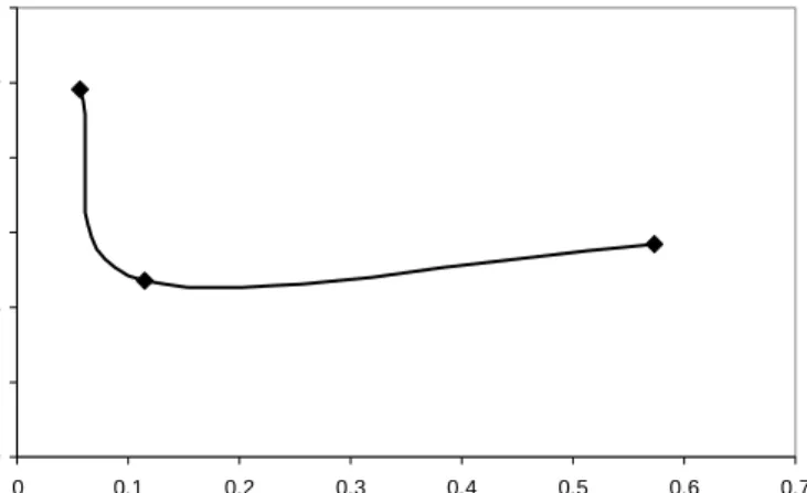
Figure 3 shows the effect of inclination angle (slope) of the channel on the outlet mass flow rate for case1 (θ=0.057°), case4 (θ=0.1145°) and case5 (θ=0.573°). It is clear that by increasing the inclination angle from θ=0.057° to θ=0.1145° the outlet mass flow rate decreases but when it increases to θ=0.573°
the mass flow rate increases. Therefore it is clear that the outlet mass flow rate is at a minimum value at a range of inclination angle of the channel.
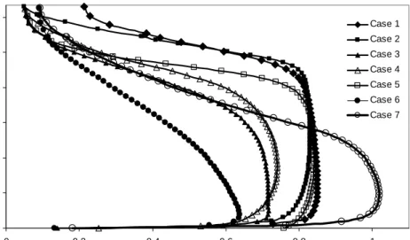
Velocity profile is considerably affected by a change in the width and slope of the channel. The effect of slope, aspect ratio of the channel and divergence and convergence of it due to change in channel width is investigated in Figure 4 at Z=0.55m and at the middle of the channel. It is seen that by increasing the aspect ratio from 0.4 to 1.2 for case1, case2 and case3 the maximum of velocity in the channel increases and is near the bed of the channel. Also it is clear that by increasing the slope of the channel from
θ=0.057° to θ=0.1145° for case1 and case4 the maximum velocity of the flow decreases but when the slope increases from θ=0.1145° to θ=0.573° the maximum velocity increases and the location of the maximum velocity moves to near the free surface of the flow that it is due to this may be attributed to accelerating flow in the channel. Also it is clear that the velocity profile is flat when the slope of the channel decreases. A very interesting result of this section is the effect of convergence and divergence channel on the velocity profile in case6 and case7. It is clear that the difference between maximum velocity at the convergence and divergence channel is very high and the velocity is at higher value for divergence channel against the convergence channel. Also it is clear that the location of maximum velocity is nearer the bed for the convergence channel.
0 2 4 6 8 10 12 0 0.1 0.2 0.3 0.4 0.5 0.6 0.7
inclination angle (degree)
M a s s fl o w r a te (kg /s)
0 0.02 0.04 0.06 0.08 0.1 0.12 0 0.2 0.4 0.6 0.8 1 velocity (m/s) De p th ( m ) Case 1 Case 2 Case 3 Case 4 Case 5 Case 6 Case 7
Figure 4. Velocity profiles along vertical direction
Figure 5 shows the volume fraction of the air at the outlet of the channel (Z=0.6m) for case1 to case7. It is clear that the depth of water at the end of the channel is higher at AR=0.8 against the AR=0.4 and AR=1.2 for case1, case2 and case3. Also it is clear that by increasing the inclination angle or slope of the channel in case1, case4 and case5 the depth of the water increases. Also a very interesting result of this section is the effect of convergence and divergence channel on the depth of water at the end of channel. It is clear that the depth of water is at lower value when the channel is divergence and it is at higher value when the channel is convergence that it is due to volume of the water at the end of channel.
0 0.1 0.2 0.3 0.4 0.5 0.6 0.7 0.8 0.9 1 0 0.02 0.04 0.06 0.08 0.1 0.12 0.14 Depth (m) V o lum e f ra c tion of a ir case 1 case 2 case 3 case 4 case 5 case 6 case 7
Figure 5. Volume fraction of air along vertical direction at outlet of channel
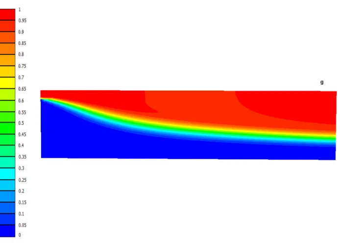
Figure 6 shows the contours of volume fraction of air for case1 to case7. It is evident that the water surface is different for different aspect ratios, different inclination angles and convergence-divergence state even in a channel with the same water depth (h =0.11 m) in the inlet. It is clear that the surface tension is moderate and allows the water surface to deform freely in space for AR=1.2 and AR=0.8. The water surface has limited freedom to deform in space when the AR=0.4, because of the strength of the inertia force. This condition is also confirmed for slope of the channel because with increasing the slope in case5 the water surface has limited freedom to deform in space. In case6 and case7 for convergence and divergence channel it is clear that the water surface has the higher value for convergence and lower value for divergence condition.
Figure 6. Contour of volume fraction of air at middle of the channel for (a) case 1, (b) case 2, (c) case 3, (d) case 4, (e) case 5, (f) case 6 and (g) case 7
4. Conclusion
A complete three-dimensional and two phase CFD model with finite volume method (FVM) and a dynamic Sub grid-scale for prediction of flow distribution in an open channel investigated. The results of this paper are in good agreement with experimental results of Knight et al.[10]. The results show that by increasing the aspect ratio of the channel the mass flow rate increases but by increasing the inclination angle from θ=0.057° to θ=0.1145° the outlet mass flow rate decreases and when it increases to θ=0.573°
the mass flow rate increases. Also it is clear that the difference between maximum velocity at the convergence and divergence channel is very high and the velocity is at higher value for divergence channel against the convergence channel.
References
[1] Hubert, C., The Hydraulics of Open Channel Flow: An Introduction, Elsevier
Butterworth-Heinemann, 2nd ed., 2004.
[2] R. Nagaosa. Direct numerical simulation of vortex structures and turbulent scalar transfer across a free surface in a fully developed turbulence. Physics of Fluids, 11(6):1581-1595, 1999
[3] V. Borue, S.A. Orszag and I. Staroselsky. Interaction of surface waves with turbulence: direct numerical simulations of turbulent open channel flow. Journal of Fluid Mechanics, 286(1): 1-23, 1995
[4] Salami L.A., “On velocity-area methods for asymmetric profiles”, University of Southampton Interim Report V, 1972.
[5] Schlichting, H., “Boundary Layer Theory”, McGraw Hill, 1979.
[6] Sooky, A. A., “Longitudinal dispersion in Open Channels”, Journal of Hydraulic Division of American Society of Civil Engineering, Engineering Vol. 95, No. 4, 1969, pp. 1327-1346.
[7] Bogle, G. V., “Stream Velocity Profiles and Longitudinal Dispersion”, Journal of Hydraulic Engineering-Trans ASCE, Vol. 123, No. 9, 1997, pp. 816-820.
[8] Deng, Z., Singh, V. P. and Bengtsson, L., “Longitudinal Dispersion Coefficient in Straight Rivers”, Journal of Hydraulic Engineering-Trans ASCE, Vol. 127, No. 1, 2004 pp. 919-927. [9] Seo, Won II and Baek, K.O., “Estimation of the longitudinal dispersion coefficient using the
velocity profiles in natural streams”, Journal of Hydraulic Engineering-Trans ASCE, Vol. 130, No. 3, 2004, pp. 227-236.
[10] D. W. Knight. Boundary shear in smooth and rough channels. ASCE, Journal of Hydraulic
Engineering, Hydrologic Science Division, 107(7):839–851, 1981
Iman Khazaee was born in mashhad, iran, in 1983. He received his B.S. degree in mechanical
engineering from Ferdowsi university of mashhad in 2006 and his master’s degree at mechanical engineering department, Amirkabir University of Technology in 2008 and a PhD degree from Ferdowsi University of Mashhad in 2011. Currently, he is working on PEM fuel cells and their optimization. E-mail address: [email protected]
Mohammad Mohammadiun was born in Shahrood, Iran, in 1977. He received his B.S. degree in
Mechanical Engineering from Khajeh Nasir Toosi University, Tehran, in 2001 and his M.S. degree in Bio-mechanics from Amir Kabir University in 2004. He has been a doctoral student in the Department of Mechanical Engineering at Ferdowsi University of Mashhad since 2008.