Models for Evaluation of Mobile Network
Functions
著者
Suzuki Masaki, Kitahara Takeshi, Ano
Shigehiro, Tsuru Masato
journal or
publication title
IEEE Transactions on Network and Service
Management
volume
15
number
1
page range
127-141
year
2017-11-16
URL
http://hdl.handle.net/10228/00006945
doi: info:doi/10.1109/TNSM.2017.2774293Group Mobility Detection and User Connectivity
Models for Evaluation of Mobile Network Functions
Masaki Suzuki,
Member, IEEE,
Takeshi Kitahara, Shigehiro Ano, and Masato Tsuru,
Member, IEEE
Abstract—Group mobility in mobile networks is responsible for dynamic changes in user accesses to base stations, which even-tually lead to degradation of network quality of service (QoS). In particular, the rapid movement of a dense group of users intensively accessing the network, such as passengers on a train passing through a densely populated area, significantly affects the perceived network QoS. For better design and operation of mobile network facilities and functions in response to this issue, monitoring group mobility and modeling the access patterns in group mobility scenarios are essential. In this paper, we focus on fast and dense group mobility and mobile network signaling
data (control-plane data), which contains information related
to mobility and connectivity. Firstly, we develop a lightweight method of group mobility detection to extract train passengers from all users’ signaling data without relying on precise location information about users, e.g., based on GPS. Secondly, based on the same signaling data and the results obtained by the detection method, we build connected/idle duration models for train users and non-train users. Finally, we leverage these models in mobile network simulations to assess the effectiveness of a dynamic base station switching/orientation scheme to mitigate QoS degradation with low power consumption in a group mobility scenario. The obtained models reveal that train users consume 3.5 times more resources than non-train users, which proves that group mobility has a significant effect on mobile networks. The simulation results show that the dynamic scheme of base station improves users’ perceived throughput, latency and jitter with small amount of additional power consumption in case of a moderate number of train users, but its ineffectiveness with larger number of train users is also shown. This would suggest that group mobility detection and the obtained connection/idle duration models based solely on control-plane data analytics are usable and useful for the development of mobility-aware functions in base stations.
Index Terms—Mobile network, Mobile data analysis, Group mobility, Utilization model, Mobile network simulation.
I. INTRODUCTION
Mobile networks are expected to provide an ever-increasing number of users with satisfactory quality of service (QoS) even in challenging environments. With meticulous analyses of growth trends and thorough planning, networks can adapt to variable and heterogeneous needs. However, as current mobile networks remain considerably static due to the high cost of temporary reshaping, they are still enable to adapt well to changes in demand that are not related to global trends but are instead dynamically caused.In general, sudden changes in de-mand are especially difficult to predict and handle efficiently,
M. Suzuki and T. Kitahara are with KDDI Research, Inc., Saitama 356-8502, Japan (E-mail: [email protected]; [email protected]).
S. Ano is with KDDI Corporation, Tokyo 102-8460, Japan (E-mail: [email protected]).
M. Tsuru is with Kyushu Institute of Technology, Fukuoka 802-8502, Japan (E-mail: [email protected])
and thus result in either QoS degradation or extra expenditure. If base stations are designed to handle peak levels of changing demand, a large proportion of the resources goes unused during normal demand periods. Otherwise, users perceive degraded QoS during the peak demand period. A typical and important example causing sudden changes in demand is the movement of dense groups of users intensively accessing the network that requires the reallocation of resources to a large number of devices at the same time. From the mobile network operator’s (MNO’s) point of view, a new solution should be developed for QoS degradation due to group mobility that emphasizes cost and energy efficiency.
As a solution for the above-mentioned issues, in this paper, we consider a dynamic base station switching/orientation scheme. The assessment of such a new scheme involves the following procedures. Firstly, group user mobility should be modeled based on monitoring, which includes detecting the movement of groups of users and analyzing/understanding the users’ utilization of the network. Then, using the results of the monitoring and modeling, an initial evaluation of the scheme should be conducted, which is needed prior to scheme deployment in the real network and directly affects the decision on deployment. However, these procedures are challenging due to the following conditions and regulations:
Difficulty of collecting accurate locations of users:
Detecting a group of users is straightforward if the accurate locations of all the users are available in general. Such information is however both difficult and/or costly to obtain and not desirable in terms of privacy issues. Therefore, the detection of moving groups of users should not require the accurate location of individual users.
Difficulty of using training-based methods: As metropolitan areas are in a state of constant evolution with, e.g., the construction of new buildings and the modification of urban facilities, MNOs must frequently adapt their networks by adding base stations and chang-ing their parameters includchang-ing the orientation of their antennas. In addition, since the radio conditions are very sensitive, the coverage of base stations relies on the weather. If a group mobility detection method relies on some training according to the network conditions, it would need incessant training phases and would not be practical. Therefore, the method should not require any form of training.
Need for frequent updates: How the network is used basically depends on how customers use their devices. Thus, network utilization/connectivity patterns are likely
to change with time as new devices and applications are released, so any analyses should be updated on a weekly or daily basis. Therefore, the detection method and consequent analyses should be lightweight.
Difficulty of collecting and handling user data: All IP traffic in LTE networks is separated into user data and control data. User data contains application data and control data contains messages for handling connections for user data. Network utilization/connectivity is often analyzed based on user data. However, user-data-based analyses generally require a large amount of processing power and time. Moreover, user data is not desirable for privacy reasons. Therefore, the analyses should function without user data.
Difficulty of on-field experiments: An on-field experi-ment with active performance test will require a number of testers who take trains carrying their own devices. While the public transportation service covers a variety of locations with different environmental conditions in a metropolitan area, such a costly experiment is difficult to conduct on all locations. Furthermore, the experiments should be repeated due to frequent changes of the en-vironmental conditions as noted above. Therefore, the process should be based on passively collected data in a lightweight manner instead of actively collected ones in on-field experiments.
In this paper, we discuss a general process consisting of the following three tasks to evaluate a resource allocation scheme relating to group mobility in mobile networks by taking into account the above-mentioned challenging requirements. Firstly, we develop a group mobility detection method using signaling data in an actual mobile network, which leverages the spatial and temporal locality dimensions passively moni-tored in the network. The location accuracy of the method only relies on the locations of base stations that are naturally figured out by MNOs. The method is not affected by changes in environmental conditions or the configuration of base stations. The method can also be validated by consistency with the ground truth of actual train timetables and train track loca-tions. Secondly, we construct connectivity models expressed by connected/idle durations. The connected/idle durations for train users and non-train users are extracted from the same signaling data used in the detection method, and are used to build and validate the models for this task. We assume that network accesses are triggered by either human activities or background applications activities, and then describe the models with a mixture of two different distributions. The models are validated in a way similar to the leave-one-out cross-validation technique. Finally, we leverage the models to conduct an initial evaluation of newly introduced functions. We assess the impact and effectiveness of a dynamic base station switching/orientation scheme in group mobility scenar-ios by network simulation. The scheme is evaluated in terms of the user-perceived QoS and additional power consumption. Since the connectivity models used in the simulation are built based on the data in a specific area and period of time, we vary the parameters of the models in order to simulate a range
of group mobility with different conditions. We can obtain a relative evaluation, e.g., results revealing the sensitivity of the scheme to the model parameters.
In the above-mentioned process, the first and second tasks based on our previous conference paper [1] and the third task are integrated to demonstrate the availability and usefulness of the detection method and the models for group mobility. The main contribution of this paper is three-fold in the application of Big Data analytics:
We develop and validate a detection method to monitor group mobility, which achieves decent performance with a precision of 0.70 and a recall of 0.75.
We build and validate connected/idle duration models for both train users and non-train users, which reveal that train users consume 3.5 times more resources than the others.
Through simulation based on the obtained models, we evaluate a dynamic base station switching/orientation scheme that dynamically adjusts base stations’ capability in synchronization with the group mobility of users. The simulation results suggest that the new scheme is feasible in real-world commercial environments. It can improve users’ perceived throughput, latency and jitter, which are 962%, 18% and 32% compared to those without the additional base stations implementing the scheme, with small amount of additional power consumption of 2.0%. The rest of this paper is organized as follows. The position of this paper is clarified in Section II. The group mobility detection method is proposed and its performance is evaluated in Section III. In Section IV, network utilization by train users and non-train users are modeled and the proposed models are validated. The availability and usefulness of the models are demonstrated by being applied to a practical use-case of the initial evaluation phase of mobile network functions in Section V. Section VI finally concludes this paper.
II. RELATED WORKS
Our work deals with mobile users communications in a metropolitan area with trains from MNO’s view point, and consists of (i) detecting the group mobility of train users; (ii) building users’ connectivity model using the results of (i); and (iii) assessing some new base station functions through simulations driven by the models obtained in (ii). As described in Section I, they face the five types of difficulties from practical conditions and regulations. In this section, related works are reviewed for each technical component, i.e., (i), (ii), and (iii), to show the appropriateness of our design choices.
A. User mobility extraction
User mobility has been extensively researched originally in the ad-hoc network field [2], [3]. [2] introduced typical mo-bility patterns and evaluated their effects on the performance of routing protocols. [3] proposed a routing-based location management scheme for wireless mesh networks. They math-ematically described clients mobility using stochastic Petri net techniques, then they evaluated their proposed method. Those
mobility models have been improved and applied to cellular networks for cell planning [4], and for mobility-aware func-tions [5], [6]. However, while those characterizafunc-tions of mo-bility are useful for creating sufficiently realistic simulations, they are not necessarily useful for monitoring or detecting the movement of groups of users in a real network in an efficient manner and for subsequently constructing connectivity models of users according to their fashion of locomotion.
Independently of ad-hoc or cellular networks, the nature of human mobility itself has been studied in [7]. [7] reported that human mobility displays similar features to Levy-walks, including heavy-tail flight and pause-time distributions and the super-diffusion followed by subdiffusion. Roughly speaking, human mobility is likely to be directed random walk rather than pure random walk. This report, however, does not include group mobility, and our objective is to label users with their way of movement.
Great efforts have been made to characterize and understand human mobility based on actual call detail records (CDR) or base station logs [8]–[12]. CDR are data records of commu-nication i.e., phone call, Internet connection, short messaging service, etc., which contain subscriber IDs of endpoints of communication, the start time, the duration of communication, etc.. Since CDR contain the privacy sensitive information such as subscriber ID, the data should be carefully treated. Base sta-tion logs are data records that contain the user device IDs and the times that they connect to the base station. It sometimes contains the radio resource control logs. In [8], by monitoring the distribution of CDR during business hours, they estimated the mobility of commuters that travel daily across the geo-graphical gap between users’ residences indicated by billing ZIP and their places of employment. They further estimated the carbon emissions and traffic volume as in transportation. [9] proposed a route classification method and showed the practical capability of deriving the trajectories using handoff patterns of CDR: not only identifying the train lines but also detecting the train tracks matching cellular handoff patterns to routes. According to their evaluation, the handoff patterns are robust and distinguishable even if small changes occur in route, speed, direction, phone model, and weather conditions. [10] proposed a human travel estimation method to specify the means of movement and the destination. To finely estimate the travel using the coarse location information of base station logs, they made use of supplementary information. An efficient pattern creation method was proposed in [11]. [11] classified the ways of movement of train users in relation to train lines, which requires training in the beginning of the classification. However, those methods are not easily applied to our analysis. This is because [8]–[11] require supplementary information such as map information, etc. In addition, [9] and [11] require a training phase with considerable overhead in the initial part of the detection process.
The concept of group mobility has been especially high-lighted since group mobility is likely to cause inefficiency of resource utilization and bursts of demand [13]–[16]. [13] introduced a variety of group movement models and evalu-ated the effect of types of group mobility on connectivity and throughput of an ad-hoc network. [14] introduced an
aggregation and separation movement model for groups of people. [15] proposed very microscopic group mobility level classification and group structure recognition for pedestrians, using sensors on the pedestrians’ smartphones. [16] took into account spatial and temporal locality dimensions using sensor data to quantify the correlation between the mobility of users. Another viewpoint regards group movement as one of many group events. Group event detection has much progressed in the participatory sensing field [17], [18]. [17] proposed a detection method for the boundaries of concurrent events to efficiently improve the quality of information and to appro-priately define the incentive for sensing. The method uses a combination of coarse- and fine-grained boundary detection but it requires accurate location information as observed by devices. [18] proposed the combination of two centralized event detection algorithms that make use of the Min-cut theory and SVM pattern matching technique. The intuition of our approach is similar to that of [18], which is “real-world events usually exhibit some spatiotemporal patterns.” However, those methods are not easily applied to our analysis. This is because the characterizations of group mobility in [13], [14] are useful for creating simulation, but are not necessarily useful for monitoring or detecting the group movement of users in real network. [15]–[18] require accurate and fine-grained location information of users but it is difficult to collect and use sensor data observed on user devices. Also, while [18] intended to deal with general events, we focus specifically on group movement. In order to eliminate the effects of behavior other than group movement, we directly make use of characteristics of group movement.
The core technique of our group movement detection is clustering. Many clustering algorithms have been developed specially for data streams where the processing speed and efficiency should be high [19]–[21]. Data streams are char-acterized as data that is generated continuously and simulta-neously by millions of devices, e.g., phone call records, and the data is usually massive amount. [19] proposed CLARA, which is based on a partitioning around medoids algorithm. In the initial part of the process, CLARA randomly chooses data samples to calculate medoid candidates then repeatedly refines the accuracy of those medoids. [20] proposed the BIRCH al-gorithm, which builds a hierarchical data structure (CF-tree) to compress the amount of data and cluster leaves with a k-means clustering algorithm. [21] proposed the STREAM algorithm, which splits the data into chunks then locally clusters the data in each chunk and extracts the center of each cluster in a rapid way (LSEARCH). After the local clustering, it globally clusters all centers using a k-means algorithm. These algorithms have a great advantage in processing speed but are not sufficiently flexible for our purpose; the clustering should provide a corresponding relationship of each resulting cluster to a way of movement. In addition, they require to estimate an appropriate number of medoids in advance. However such an estimation is difficult since we do not know accurate train movement schedule all the time. It is also too time- and resource-consuming to introduce the appropriate number of medoids with an optimization function such as the Silhouette value [22].
B. Network connectivity modeling
For users’ behavior analysis, user-plane data is often used. User-plane data is any data directly generated by user ap-plication, i.e., audio, video, text and so. Although it can be used to analyze the traffic volume, the time duration, and the transferred contents of each user activity, it often requires a large amount of processing power and time. Moreover, since user-plane data usually contains privacy sensitive data, it is necessary to obtain users’ permission for analysis. A number of studies for user connectivity modeling are found in literature [23]–[25]. [23] analyzed traffic patterns using cellular base station trace data. They revealed the traffic patterns depending on cell-towers, the geographical context of traffic patterns. Then, they modeled the traffic patterns in terms of their time domain and frequency domain aspects. [24] analyzed user data on the commercial 3G network and defined categories of machine-to-machine devices. They investigated daily and weekly patterns of the traffic volume, frequency of data generation, geographical distribution, comparison with smartphones, application usage, and network performance. [25] deeply investigated the events which put a temporally but extremely high demand for communication capacity on cellular networks with commercial voice and data traces. They revealed the performance degradation both pre- and post-connection, then proposed and evaluated an adequate mitigation method.
On the other hand, a number of studies using control-plane data are also found in literature [26]–[28]. Control-plane data, also known as network signaling data, is convenient and useful for MNOs. This is because it consists of very smaller volume compared with user-plane data, is easy to retrieve from a mobile network perspective, and contains information related to the mobility and the connectivity of all mobile devices. Compared with user-plane data, analyses based on control-plane data are expected to be fast and practical. Analyses based on control-plane data have been studied to investigate the interactions of control-plane protocols [26], so as to improve the management of mobility [27] and even to evaluate the effect of a signaling storm on a mobile network [28].
The approach proposed in this paper is based on monitoring and analyzing control-plane data. This is firstly because we cannot analyze user-plane data due to both of computing resource and privacy issues. Secondly, we just focus on users mobility and connectivity and are not interested in user content or very microscopic users’ behavior. Furthermore, we uniquely focus on the difference of users’ connectivity corresponding to the users’ way of movement, which requires sufficiently wide area of data but its analysis should be sufficiently fine-grained. To the best of our knowledge, this is the first challenge to investigate user connectivity models based solely on network signaling data that are captured behind base stations. The proposed network connectivity models for train and -non-train users are explained in detail in Section IV.
C. Network simulation and assessment for network functions
To quantitatively analyze and assess a complicated system in a specific circumstance, simulation-based evaluation is
es-sential in many cases where in-lab experiments are not at scale and real-world experiments are too costly. In particular, it is of practical importance to initially assess some system functions with parameter tuning by simulation before development and deployment of the functions. In general, there are two types of simulation; model-driven simulation that uses simulation-input data generated from models built and tuned for the targeted environment [5], [6], and trace-driven simulation that uses simulation-input data generated from actual data obtained from real experiments [4], [25]. Model-driven simulation can be easily applied to any form of simulation but its adequateness depends on how well the model reflects the reality. While it possibly includes a gap between simulation and real world so that it usually requires on-field experiments afterwards, model-driven simulation is suitable for the initial evaluation with synthetic simulation. [5] evaluated the effects of adaptive virtual network function on the changes of latency with varied speed of user devices. [6] evaluated the accuracy of mobility estimation using linear dynamic system model of mobility.
On the other hand, trace-driven simulation is capable of real-istic simulation by conducting the actual users’ behavior but is not likely to be flexible to apply to general simulations. Thus, it is difficult to verify the generality of simulation results. [4] computed pseudo-user mobility in order to evaluate cell planning efficiency using a census data for user movement in specific but relatively large area. [25] evaluated the congestion mitigation schemes using the actual radio resource control logs and TCP header in data traffic, which are observed in the specific events, i.e., football games, and public demonstrations. In this paper, we evaluate the mitigation methods for QoS degradation caused by user mobility through simulation based on train and non-train users connectivity models. To inves-tigate how the mitigation methods generally impact on the fundamental network performance, we conduct a synthetic simulation. Therefore, we cannot directly apply the actual trace-data to simulation and, instead, we apply the connectivity model based on actual signaling data. In order to mitigate QoS degradation caused by mobility or group mobility, a variety of adaptive functions have been proposed [5], [6], [29]–[31]. To enhance the conventional base stations that are designed to have sufficient resources for peak demand periods and are always on even in normal demand periods, [29] proposed a smart scheme to switch on/off the base stations depending on the traffic load in order to reduce extra power consumption. The scheme could reduce the power consumption by 60% on weekdays and by 80% on weekend. [30] introduced the fundamental idea of moving antenna to steer the orientation of antenna targeting a moving user device. [31] further developed the idea of dynamic orientation focusing on a high speed train scenario. It discovered a new type of spatial-temporal correlation between the base station and moving antenna on the roof-top of train. We define dynamic base station functions essentially based on the ideas discussed in [29] and [30] as we call dynamic base station switching/orientation scheme hereafter. We evaluate the fundamental performance metrics with two dynamic base station functions: dynamic switch on when trains come close and switching off when they go, dynamic orientation of directional antenna tracing the group
Fig. 1. Simplified LTE network architecture.
movement in Section V.
III. SIGNALING-BASED GROUP MOBILITY DETECTION
We propose a group mobility detection method consisting of three steps: signaling data analysis, handover clustering, and moving group extraction. The core idea of our group mobility detection lies in the fact that users moving together will often change the associated base station at the same time and around the same location. The first step in this method is to detect changes of base station by users, called handover events. The second step aims to identify groups of users by clustering these handover events by location and time. The locations here do not correspond to users’ locations but to the locations of base stations. Finally, by taking advantages of the time dimension to filter and gather the clusters, we can retrieve the users moving together over time with a high-level of confidence.
A. Signaling data analysis
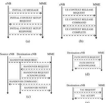
When devices move or access the network, control-plane signals are triggered aiming at the management of mobility and connectivity. By capturing and analyzing these signals, we can obtain access information about the mobile network and its devices without interfering with the network entities themselves. Our analysis focuses on the control signals carried over theS1-MMEinterface of the LTE architecture, described in Fig. 1. Located between the evolved NodeBs (eNBs), i.e., the base stations of LTE networks, and the mobility manage-ment entity (MME), this interface uses the S1 Application Protocol (S1AP) [32] to carry signals related to connectivity and mobility.
Each time an idle device tries to access the network, a sequence of three messages described in Fig. 2(a) is exchanged between its serving eNB and the MME. When a connected device causes use of the network, it returns to an idle state after the exchange of a sequence of three other messages, described in Fig. 2(b). Analyzing these two sequences of messages allows us to detect when a device goes connected or idle, and thus to determine the connectivity state of the device. In order to improve the strength of the radio signals, a connected device can change the serving eNB by performing a
handover. These phenomena frequently occur when users are moving and can be split into two categories according to the way in which the process is executed:X2-handovers, in which the process is performed almost entirely between the two eNBs, and S1-handovers, in which the process is performed by the MME. The mobility of connecteddevices can thus be
(a) (b)
(c)
(d)
(e)
Fig. 2. S1AP signals related to connectivity and mobility. Signals related to connectivity are described in (a) and (b). S1-handover signals, X2-handover signals, and TAU signals are respectively detailed in (c), (d) and (e).
determined by detecting the handovers. Besides, in order for the mobile network to be able to redirect mobile-terminated calls and packet transfers using paging, the evolved packet core (EPC) must remember the tracking area (TA), i.e., the group of eNBs, containing the eNB last contacted by the device. When a device changes TA, a signaling procedure called atracking area update (TAU) is emitted on the S1-MME interface to notify the EPC, even when the device is idle. The messages related to handovers and TAUs that we analyze in our method are detailed in Figs. 2(c), 2(d), and 2(e).
Although enormous, the volume of signaling data is rela-tively small compared with user-plane data. Our implementa-tion in C/C++ shows that it is possible to finish analyzing the numbers of S1AP packets faster than the rate of data acquisition. We output events related to the connectivity of the devices to queue Cq and events related to mobility to queue
Mq. As all mobility events represent a change of base station
from source base station sa to destination base station da,
all mobility events will now be called handover events. Each handover event will be denoted byh psa, daq.
B. Handover clustering
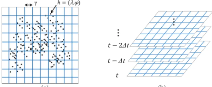
The second step of the detection method is responsible for revealing the movement of groups of users by clustering the previously computed handover events by location and time. We definepλ, ϕqas the location of handover h psa, daqas the
middle point ofsa andda, whereλandϕrespectively refer to
the longitude and latitude ofh.pλ, ϕqis a rough approximation of the location of the device initiating the handover.
At each timet k∆t pk PNq, with ∆t being a constant interval in seconds, we remove and retrieve all the handovers currently present in Mq and cluster their locations using a
(a) (b)
Fig. 3. Handover clustering. The clustering realized at one specific time is illustrated in (a), and (b) represents the sliding window storing the clusters of several times.
longitudes and latitudes λmin, λmax, ϕmin, and ϕmax. Let
r rpϕmaxϕmin{γs, and c rpλmaxλminq{γs be the
number of rows and columns of the grid andnrcthe num-ber of clusters, respectively. Clusters Cptq pC0, . . . , Cn1q
computed at timet are defined in Eq. (1).
Ci " hPMq Zλλmin γ ^ r Z ϕϕmin γ ^ i * . (1) This clustering method is primitive. However, since the locations of handovers are particularly rough, our method can be useful without more sophisticated clustering. It also has the advantage of being linear in the number of handovers, which preserves the processing speed of the method. Figure 3(a) illustrates the clustering realized at time t. A sliding window
W pCpt i∆tqqP i¤0of sizeP PNis shown in Fig. 3(b). The values of∆tandγhave a direct impact on the size of the clusters and the frequency at which they are computed, which will be discussed in more detail in Section III-D.
C. Moving group extraction
Let us define the following relation between devices: two devices uandv areclustered togetherat timetif and only if
they initiate handovers that are located in the same cluster at t. Due to the roughness of the handover locations and the irregular accesses to the network by different devices, two devices actually moving together may not always initiate handovers at the same time and same location and thus may not always beclustered together. Besides, two devices crossing paths may at some point initiate handovers at the same location and same time and thus may be wronglyclustered together. In the last step of the detection method, we use sliding window
W to filter and merge clusters in order to only retrieve groups of devices truly moving together.
We define Gptq pG1, G2, . . .q as the list of groups of devices truly moving together at time t. We decide that two devices are actually moving together if and only if they are clustered together at least N times out of P, where
N P t1, . . . , Pu is a constant parameter. At time t and for each pair of devices tu, vu, we retrieve from W the lists of clusters Cu pCu,t i∆tqandCv pCv,t i∆tqthat uandv
have been clustered in for P i ¤ 0. We then compute
Ncom |CuXCv|, the number of clusters that are common
inCu andCv. Lettf irst¤tandtlast¤tbe the times of the
Fig. 4. Group extraction withP 3andN2. For instance, device is in the same clusters as device⋆Ncom2times andNcom¥N; therefore,
they are considered to be moving together att2∆t,t∆t, andt.
first and last common clusters, if they exist. If Ncom ¥ N,
we consider that uandv were truly moving together during intervalrtf irst, tlastsand thus we put them in the same group
of devices for each timetgP rtf irst, tlasts. This implies that
groups Gptf irstq are modified at time t ¥tf irst: groups of
previous times can be modified as new clusters are computed. This choice is correctly made to gather devices that have just started to move together and cannot otherwise be considered to be moving together. Figure 4 illustrates this step with
P 3 andN 2: each geometrical symbol represents the handovers initiated by one device, each large square represents one cluster, and the dashed ellipses show which devices are truly moving together. As and▲are in the same clusters as
⋆,■, and▼at timest2∆t, andt, we haveNcom2and
asNcom¥N 2, they are considered to be moving together
att2∆t,t∆t, andt. By repeating the same procedure for all devices, groups of devices moving together are extracted and the result is depicted on the right-hand side of Fig. 4.
The groups of devices extracted at time tP∆t can be modified until t and thus can only be fully determined at t. This induces a delay of d P∆t, which is the theoretical limitation of our approach. This delay is irrelevant to our current objective but could be important in other applications. At timet, we add the list of groups of devicesGptP∆tqto queueGq. At the end of this final step, Gq contains for each
timetk∆t pkPNqlist Gptq of groups of devices moving together att.
D. Evaluation and discussion
As our objective is to detect dense moving groups of users for network performance evaluation, we incorporate our method into an actual LTE network and evaluate its perfor-mance by applying it to the detection of train movements. The location of a detected group of devices can be approximated by the average location of the handovers it contains. Comparing the locations of the detected groups with real train locations allows us to evaluate the method. Using train timetables and train track locations, we estimate the locations of real trains at each timet. LetAptqbe the set of real trains present in the considered area at time t and let pat,1, . . . , at,|Aptq|qbe their
actual locations. We filter Gptq to only keep large groups of devices, whose locations are denoted by pdt,1, . . . , dt,|Gptq|q.
We match pat,1, . . . , at,|Aptq|q and pdt,1, . . . , dt,|Gptq|q using
Fig. 5. Precision and recall according to the time of day.
between each matched location. Matched locations represent detected groups that are located near real trains, i.e., true positives, and unmatched locations represent either detected groups located far from any real train, i.e., false positives, or real trains that have not been detected, i.e., false negatives. Let Mptq be the set of matched locations; we can compute the precision, the recall, and F-measureF1 of the method for each time tas shown in Eqs. (2) and (3).
precisionptq |Mptq| |Gptq|, recallptq |Mptq| |Aptq|, (2) F1ptq 2precisionptq recallptq precisionptq recallptq. (3)
This evaluation is realized on the actual anonymized control-plane data corresponding to a period of four weeks in a large metropolitan urban area in Japan. A total of 25 billion packets are analyzed, trains are detected, and their locations are evaluated. The data used were captured at a specific area and period of time but the area and period are sufficiently typical in terms of human activities. Figure 5 shows the average performance of our method according to the time of day with the parameters described in (4). These values were chosen as they gave the best results amongst a wide range of parameters. Except in the early morning, the results show that our method achieves decent performance with a precision of 0.70 and a recall of 0.75. Considering the roughness of the handover locations, this performance is satisfactory and sufficient for further statistical analyses. The drop in recall between 5 a.m. and 7 a.m. is due to the small number of people during that period of the day: fewer people leads to fewer devices clustered together and thus fewer detected groups. The recall increases progressively between 5 a.m. and 7 a.m. as more and more people are present in the area. This issue is irrelevant to our objective as we focus on challenging situations for mobile networks and are only interested in the busiest periods of the day (between 7 a.m. and midnight).
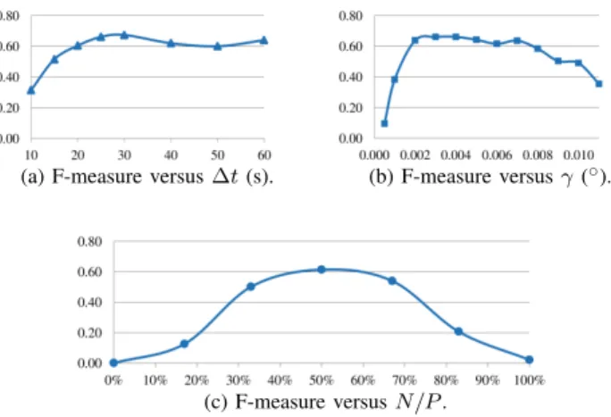
∆t30s, γ0.003, P 8, N 4. (4) To determine the best parameters for the method, we choose the F-measure as a balanced metric, i.e., the performance, to
(a) F-measure versus∆t(s). (b) F-measure versusγ().
(c) F-measure versusN{P. Fig. 6. Influence of the parameters on the performance.
evaluate both the precision and the recall according to the parameters. Figures 6(a), (b), and (c) respectively illustrate the influence on the performance of∆t,γand the performance of ratioN{P representing the proportion of time that two devices must be clustered together to be considered to be actually moving together. When ∆t is small, devices have less time to move between two clustering steps and they thus trigger fewer handovers, which reduces their chance of being clustered with other devices and leads to a drop in performance. A high value increases the number of handovers and thus the performance but also increases the delay d P∆t of the method.γ directly affects the size of the clusters: too small a value will result in extremely small clusters and fewer devices will be clustered together, whereas too high a value will result in disproportionate clusters including devices that do not move together. Finally, N{P represents the minimum similarity of the movements of two devices moving together. A good balance must be chosen as a low similarity will incorrectly mix together devices moving differently, while a high similarity will only group together devices that always trigger handovers at the same time, leading to great precision but low recall and thus low performance. With these considerations in mind, we evaluated our method for a wide range of parameters and selected the best set of parameters introduced in (4).
As our method relies solely on the base stations contacted by the users, it does not require the accurate locations of the users and it can be generalized to any type of mobile network. Fur-thermore, it does not necessitate any training phase depending on the base stations and thus works even if the topology of the network is modified. The processing delaydP∆t4min induced by the method is insignificant because the following analyses described in Section IV are expected to be updated on a weekly or daily basis. Moreover, the volume of data is large enough to include diverse information and to allow reliable analyses based on the data. Therefore, the proposed detection method fulfills the conditions and regulations described in Section I, and is applicable to the following analyses.
IV. SIGNALING-BASED USERS’CONNECTED/IDLE DURATION MODELS
We propose users’ connected/idle duration models based on signaling data to estimate user-level network utilization by the
Fig. 7. Relation between observed durations and actual durations.
detected moving groups of users. We call users detected by our detection method train users and all the other non-train users. We then model the time spent using the network by each user.
A. Users’ connected/idle duration models
Network utilization time can be estimated by the durations of connected and idle states of each user. We retrieve the connectivity events stored in queue Cq defined in III-A and
compute the list of connected/idle durations of each device. Using our group mobility detection method, all users are divided into train users and non-train users. Four different durations are recorded in listsDCT,DCN T,DIT, andDIN T
containing respectively the durations ofconnected train users
(CT),connected non-train users(CNT),idle train users(IT), and idle non-train users (INT). As mobile networks use a timeout to detect the inactivity of users, a device does not actually use the network for the duration of this timeout and network utilization is thus better approximated by subtracting the value of the timeout from the observed connected duration. In addition, a device does not actually use the network while it is establishing a connection. We estimate the connected/idle durations in our model from the observed durations as illus-trated in Fig. 7.
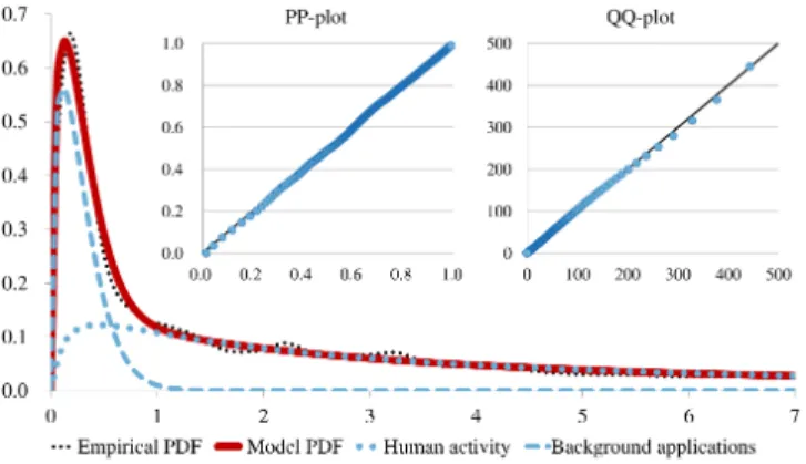
The probability density functions (PDFs) of the durations contained in each list are estimated using a kernel density es-timation (KDE) [34] with Gaussian kernel Kexp x2{2
and bandwidth h 0.1s. If pd1, . . . , dnq are n durations,
the empirical PDF f˜of the distribution of their durations is computed as in Eq. (5). Figure 8 illustrates the empirical PDF of the CNT distribution. ˜ fpxq 1 nh n ¸ i1 K xdi h . (5) Some network accesses are caused by the diverse com-munication activities of users, generally with relatively long durations. Some other network accesses are triggered by back-ground applications causing an exchange of small amounts of data in a short duration, e.g., to retrieve the latest news, to check for emails, or to receive notifications from a server. Therefore, we model the CT and CNT distributions using a mixture of one log-normal distribution representing human activityand one Weibull distribution representing background applications.
Idle durations are directly linked with the inactivity of users but are also affected by the activity of other users. Indeed, if
Fig. 8. CNT model: empirical PDFf˜CN T, the two components of the model,
and the model PDFfCN T according to the connected duration (in seconds).
The PP-plot and QQ-plot evaluating the model are also depicted.
two users A and B are texting each other and user A sends a message to user B before going to idle, user B’s answer will activate user A and the idle duration of user A will be closed in a short time. This phenomenon is intensified by the inactivity timeout we previously mentioned: if the inactivity timeout equals 5s and user B takes 6s to reply, user A will stay in idle for 1s only. Therefore, we also model the IT and INT distributions using a mixture of one log-normal distribution for human inactivity and one Weibull distribution for idle durations closed by other user activities and applications.
We choose the log-normal distribution that is often used in the description of natural phenomena with a relatively long tail. The Weibull distribution is chosen as it fits peaks well.
Let fCT, fCN T, fIT, and fIN T be the PDFs of these
models. The common equation for them is described in Eq. (6), whereσandµare the log-normal parameters,kandλare the Weibull parameters, andαis a weighting factor between the two components. fpxq α 1 xσ?2πexp plnpxq µq2 2σ2 p1αqk λ x λ k1 exp x λ k . (6)
Let F be the cumulative distribution function (CDF) of f
andF˜ be the CDF of empirical PDFf˜. The five parameters of each model are determined by maximizing the objective function described in Eq. (7), where X pσ, µ, k, λ, αq is the vector of the parameters, and S is a dataset of samples of the duration. RP2, RC2, and RQ2 are the coefficients of
determination respectively indicating: how well PDF f fits PDFf˜, how well CDFF fits CDFF˜ (PP-plot), and how well the quantiles off correspond to the quantiles off˜(QQ-plot). This process is chosen for the model PDF with parametersX
to fit the shape of the empirical PDF derived from samples
S well, quantified by the coefficient of determination RP2
of two PDFs, while conserving the same statistical properties as the data, quantified by RC2 and RQ2. As the PP-plot
(quantified by the coefficient of determination RC2 of two
CDFs) magnifies errors in the center of the distribution and the QQ-plot (quantified by the coefficient of determination RQ2
Sat Sun Mon Tue Wed Thu Fri Sat Sun Mon Tue Wed Thu Fri Sat Sun Mon Tue Wed Thu Fri Sat Sun Mon Tue Wed Thu Fri Sat Sun Mon Tue Wed Thu Fri Sat Sun Mon Tue Wed Thu Fri
Sat 0.9950.9950.9950.9960.9960.9960.9950.9950.9950.9960.9950.9950.9950.995 Sat 0.9780.9740.9710.9710.9720.9700.9680.9780.9770.9700.9680.9680.9660.968 Sat 0.7420.7220.7580.7680.7760.7670.7620.7400.7230.7460.7730.7570.7730.764
Sun0.9950.9950.9950.9950.9960.9960.9950.9950.9950.9950.9950.9950.9950.995 Sun0.9740.9770.9560.9560.9580.9540.9510.9730.9760.9540.9520.9510.9470.950 Sun0.7380.7180.7540.7640.7720.7630.7580.7360.7190.7420.7690.7540.7690.760
Mon0.9950.9950.9960.9950.9960.9960.9950.9940.9930.9950.9950.9940.9950.995 Mon0.9700.9590.9790.9790.9790.9790.9790.9710.9630.9790.9790.9790.9780.979 Mon0.7560.7360.7720.7810.7900.7800.7760.7540.7360.7600.7860.7700.7870.778
Tue0.9950.9950.9950.9960.9960.9960.9960.9950.9940.9960.9950.9950.9950.995 Tue0.9700.9590.9790.9790.9790.9790.9790.9700.9630.9790.9790.9790.9790.979 Tue0.7470.7270.7630.7720.7810.7710.7670.7450.7270.7510.7770.7620.7780.769
Wed0.9950.9950.9950.9960.9960.9960.9950.9950.9950.9960.9950.9950.9950.995 Wed0.9690.9590.9780.9780.9780.9780.9770.9720.9650.9780.9780.9770.9770.977 Wed0.7460.7260.7620.7710.7800.7700.7660.7440.7260.7500.7760.7610.7760.768
Thu0.9950.9950.9950.9960.9960.9960.9950.9950.9940.9950.9950.9950.9950.995 Thu0.9690.9580.9790.9790.9790.9790.9790.9700.9620.9790.9790.9790.9790.979 Thu0.7470.7280.7630.7730.7810.7720.7680.7460.7280.7520.7780.7630.7780.770
Fri 0.9950.9950.9950.9960.9960.9960.9960.9950.9940.9960.9950.9950.9950.995 Fri 0.9680.9570.9790.9790.9790.9790.9790.9690.9610.9790.9790.9790.9790.979 Fri 0.7480.7280.7640.7730.7820.7720.7680.7460.7280.7520.7780.7630.7790.770
Sat 0.9950.9950.9940.9950.9960.9950.9950.9950.9950.9950.9950.9950.9950.995 Sat 0.9770.9710.9720.9720.9730.9710.9690.9780.9760.9710.9690.9690.9660.968 Sat 0.7370.7170.7530.7630.7710.7620.7570.7360.7180.7420.7680.7530.7680.759
Sun0.9950.9950.9930.9940.9950.9950.9940.9950.9950.9940.9950.9950.9940.994 Sun0.9770.9740.9630.9620.9640.9600.9580.9760.9770.9610.9580.9580.9540.957 Sun0.7270.7080.7440.7550.7620.7530.7480.7270.7100.7330.7600.7450.7590.750
Mon0.9950.9950.9950.9960.9960.9960.9960.9950.9940.9960.9960.9950.9950.995 Mon0.9690.9580.9790.9790.9790.9790.9790.9690.9610.9790.9790.9790.9790.979 Mon0.7440.7240.7600.7690.7780.7680.7640.7420.7240.7480.7740.7590.7750.766
Tue0.9950.9950.9950.9950.9960.9950.9950.9950.9950.9950.9960.9960.9960.995 Tue0.9680.9570.9790.9790.9790.9790.9790.9690.9600.9790.9790.9790.9790.979 Tue0.7330.7130.7500.7600.7680.7580.7540.7320.7140.7380.7650.7490.7650.756
Wed0.9950.9950.9940.9950.9950.9950.9950.9950.9950.9950.9960.9960.9950.994 Wed0.9680.9560.9780.9790.9780.9790.9790.9680.9590.9790.9790.9790.9790.979 Wed0.7280.7080.7450.7550.7630.7530.7490.7270.7090.7330.7600.7440.7600.751
Thu0.9950.9950.9950.9950.9960.9950.9950.9950.9940.9950.9960.9960.9960.995 Thu0.9670.9540.9780.9780.9780.9790.9790.9670.9580.9790.9790.9790.9790.979 Thu0.7360.7160.7520.7620.7710.7610.7570.7340.7170.7410.7670.7520.7680.759
Fri 0.9950.9950.9950.9960.9960.9960.9960.9950.9940.9960.9950.9950.9950.995 Fri 0.9680.9560.9790.9790.9780.9790.9790.9680.9600.9790.9790.9790.9790.979 Fri 0.7480.7280.7640.7730.7820.7720.7680.7460.7290.7520.7790.7630.7790.770
Sat Sun Mon Tue Wed Thu Fri Sat Sun Mon Tue Wed Thu Fri Sat Sun Mon Tue Wed Thu Fri Sat Sun Mon Tue Wed Thu Fri Sat Sun Mon Tue Wed Thu Fri Sat Sun Mon Tue Wed Thu Fri
Sat 0.9910.9910.9870.9870.9870.9870.9860.9910.9910.9870.9870.9860.9880.989 Sat 0.9820.9820.9810.9810.9810.9810.9800.9820.9820.9810.9800.9800.9800.981 Sat 0.5680.5590.5870.5920.5900.5920.5920.5750.5650.5890.5940.5950.5930.590
Sun0.9910.9910.9870.9870.9870.9870.9860.9910.9910.9870.9870.9860.9880.989 Sun0.9820.9820.9800.9800.9790.9790.9790.9810.9820.9790.9780.9780.9790.979 Sun0.5620.5530.5820.5870.5850.5870.5870.5690.5590.5830.5880.5890.5880.585
Mon0.9890.9890.9890.9890.9890.9890.9880.9890.9890.9880.9880.9880.9890.988 Mon0.9790.9780.9830.9830.9830.9830.9820.9800.9780.9820.9820.9820.9820.982 Mon0.5680.5600.5900.5960.5930.5950.5950.5760.5650.5910.5970.5970.5960.592
Tue0.9890.9890.9890.9890.9890.9890.9880.9890.9890.9880.9880.9880.9890.988 Tue0.9860.9840.9890.9890.9890.9890.9890.9880.9850.9890.9890.9890.9890.988 Tue0.5650.5570.5880.5940.5910.5930.5920.5730.5620.5890.5940.5950.5930.590
Wed0.9890.9890.9890.9890.9890.9890.9880.9890.9890.9890.9890.9880.9890.988 Wed0.9800.9770.9840.9840.9830.9830.9830.9800.9780.9830.9830.9830.9830.983 Wed0.5630.5540.5860.5910.5890.5900.5900.5700.5600.5870.5920.5930.5910.588
Thu0.9890.9890.9890.9890.9890.9890.9880.9890.9890.9880.9880.9880.9890.988 Thu0.9790.9770.9830.9830.9830.9830.9820.9800.9780.9820.9820.9820.9830.982 Thu0.5660.5580.5880.5940.5920.5930.5930.5740.5640.5900.5950.5950.5940.591
Fri 0.9880.9890.9880.9890.9890.9880.9880.9880.9890.9890.9890.9880.9890.988 Fri 0.9790.9770.9830.9830.9820.9820.9820.9800.9780.9810.9820.9820.9820.982 Fri 0.5550.5460.5780.5840.5820.5830.5830.5630.5520.5800.5850.5850.5840.580
Sat 0.9910.9910.9870.9870.9870.9870.9860.9910.9910.9870.9870.9860.9880.988 Sat 0.9820.9800.9820.9810.9810.9810.9800.9820.9810.9800.9800.9800.9810.981 Sat 0.5650.5570.5840.5900.5880.5890.5890.5720.5620.5860.5910.5920.5900.588
Sun0.9900.9910.9870.9870.9870.9870.9860.9910.9910.9870.9870.9860.9880.989 Sun0.9820.9820.9810.9810.9810.9800.9800.9820.9820.9800.9790.9790.9800.980 Sun0.5570.5490.5780.5830.5810.5830.5830.5650.5550.5790.5840.5850.5840.581
Mon0.9890.9890.9880.9890.9890.9880.9880.9890.9890.9890.9890.9880.9890.988 Mon0.9800.9780.9840.9840.9830.9830.9830.9800.9790.9830.9830.9830.9830.983 Mon0.5550.5470.5780.5840.5810.5830.5820.5630.5520.5790.5850.5850.5840.580
Tue0.9890.9890.9890.9890.9890.9880.9880.9890.9890.9890.9890.9880.9890.988 Tue0.9790.9770.9830.9830.9820.9830.9820.9800.9780.9820.9820.9820.9820.982 Tue0.5590.5500.5820.5870.5850.5860.5860.5660.5560.5830.5880.5890.5870.583
Wed0.9880.9890.9880.9890.9890.9880.9880.9880.9890.9890.9890.9880.9890.988 Wed0.9790.9760.9820.9830.9820.9820.9820.9790.9770.9810.9820.9820.9820.982 Wed0.5580.5490.5810.5870.5840.5860.5850.5650.5550.5820.5870.5880.5860.583
Thu0.9900.9900.9880.9880.9880.9880.9880.9900.9900.9890.9880.9880.9890.989 Thu0.9790.9770.9830.9830.9820.9820.9820.9800.9780.9820.9820.9820.9820.982 Thu0.5580.5500.5800.5860.5840.5850.5850.5660.5560.5820.5870.5880.5860.583
Fri 0.9900.9910.9880.9880.9880.9880.9870.9900.9900.9880.9880.9870.9890.989 Fri 0.9800.9780.9830.9830.9820.9820.9820.9800.9790.9810.9820.9820.9820.982 Fri 0.5590.5510.5800.5860.5830.5850.5850.5660.5560.5810.5860.5870.5860.583
CT vs CNT
IT vs INT
CT CNT
IT INT
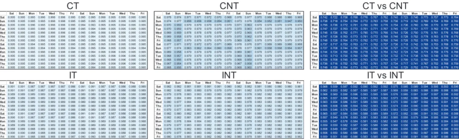
Fig. 9. Evaluation of the CT, CNT, IT, and INT models. Each row shows how well the model computed from one day’s worth of data fits the data of all the other days. Light areas represent good fitting and dark areas poor fitting.
TABLE I
MODELS:PARAMETERS AND EVALUATION.
σ µ k λ α RP2pXq, Sqq RC2pXq, Sqq RQ2pXq, Sqq objpXq, Spqq
CT 1.31 2.44 1.32 0.34 0.86 0.985 0.999 0.999 0.994 CNT 1.59 1.72 1.35 0.30 0.77 0.962 0.999 0.999 0.987 IT 0.73 3.65 1.08 6.16 0.42 0.970 0.999 0.996 0.988 INT 1.65 3.34 1.21 1.93 0.87 0.981 0.990 0.978 0.983
of two sets of quantiles) magnifies errors in the tail of the distribution, their association is expected to be effective.
objpX, Sq 1
3pRP
2pX, Sq R
C2pX, Sq RQ2pX, Sqq. (7)
We build four types of duration models for CT, CNT, IT, INT, based on fourteen days’ worth of data of duration samples coming from the same dataset used in evaluating the group mobility detection method as described in Section III-D, which consists of different days of the week. Let Spq be the
samples of date pand type q P tCT, CN T, IT, IN Tu, and
Sq
¤
p
Spq. To build a good model for given type q, we
determine parameters Xq so as to maximize the objective
function as Eq. (8). Maximization is performed using the L-BFGS-B algorithm [35].
Xq argmax X
objpX, Sqq. (8)
As there are fewer train users than non-train users, this corresponds to about 1 million samples each for the CT and IT models and25million samples each for the CNT and INT models for each day. Table I shows the parameters and the averaged fitting performance of the most general models for CT, CNT, IT, and INT, respectively. Figure 8 shows the two components of the CNT model, its PDF, PP-plot, and QQ-plot. The PDFs of the four models are depicted in Fig. 10(a) and will be discussed in IV-C.
B. Evaluation of the models
In order to evaluate our models and their computation process, we use an approach similar to the leave-one-out cross-validation technique used in statistical model cross-validation [36].
For each day of our dataset, we compute a model using this day’s worth of data and then evaluate how well it fits the data of all the other days. This allows us to ensure that the computed models do not overfit the data. The evaluation is performed on two weeks of data using the objective function,
objpXpq, Sp1q1q whereXpq is the maximized parameters (9)
for date p andq P tCT, CN T, IT, IN Tu, Sp1q1 is the
com-parison samples of datep1 andq1P tCT, CN T, IT, IN Tu.
Xpqargmax X
objpX, Spqq. (9)
Figure 9 shows the values of the objective function for each model type, where one row represents the evaluation of one day’s model by all the other days. The values are shown by indicating the gradient of intensity from obj ¤0.8 (dark) to
obj 1.0 (light). The average value is 0.995 for CT, 0.969 for CNT, 0.988 for IT, and 0.981 for INT. As a comparison, the two last tables of Fig. 9 show the results obtained when evaluating the CT models with the CNT data (average of 0.755) and when evaluating the IT models with the INT data (average of 0.578) and show that these models are very different.
We can deduce from these results that, independently of the day, all models fit remarkably well the data of all other days. This proves that our models are generalized well to other datasets and thus that they do not overfit the data. Also, the slightly darker areas that can be observed in the CNT table correspond to Saturdays and Sundays. As their evaluation averages 0.965, although these models still fit the data, it is suggested that the behavior of users on weekend is slightly different from weekdays.
(a)
(b) (c)
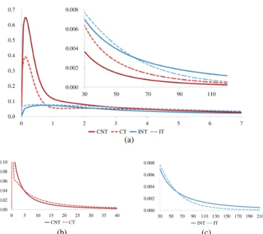
Fig. 10. (a) shows the PDFs of the CNT, CT, INT and IT models for durations in r0s,7ssand r30s,120ss. (b) shows the CNT and CT PDFs between 0s and 40s. (c) shows the INT and IT PDFs between 30s and 210s.
C. Discussion
Figure 10(a) shows that connected duration distributions have an important peak of short durations corresponding to background applications, whereas idle duration distributions are much more driven by human behavior and look like log-normal distributions. Idle duration distributions also contain a significant proportion of long durations (more than 1 min), corresponding to periods when users are not using their device at all.
Let us now compare the models for train users and non-train users in order to determine the influence of a moving group of users on the mobile network. Figure 10(b) shows that CNT contains proportionally more durations between 0s and 4s than CT and fewer between 4s and 8. Moreover, the short-durations peak is higher in CNT than in CT. This means that, not on a train, more accesses to the network are made by background applications or correspond to quick accesses by users, for example to check for new messages or briefly consult an application. On a train, however, accesses generally last longer, for instance to browse the web or watch a video. This means that users tend to use their devices more on a train, which can be explained by the fact that they have more time to spare, especially when commuting. As shown in Fig. 10(c), a train trip contains more durations between 0s and 60s than INT and fewer between 60s and 8. As short idle durations correspond to frequent network accesses and long idle durations correspond to sparse network accesses, this means that users tend to access the network more frequently on a train.
Let µCT, µCN T, µIT, and µIN T be the means of these
distributions: we obtain µCT 22.7s, µCN T 15.2s,
µIT 24.5s, and µIN T 96.3s. As devices constantly
alternate between one connected duration and one idle du-ration, the activity of users can be modeled as the couple of
random variables pC, Iq with C CT, I IT for train users and C CN T, I IN T for non-train users. The proportion of time that train users spend connected is thus
µCT{pµCTLµITq 48.1 % and the proportion of time
non-train users spend connected is µCN T{pµCN T µIN Tq
13.6 %. We deduce from these values that train users are about 3.5 times more active than non-train users. A large group of moving users will therefore have 3.5 times more impact on network resources than the same number of non-moving users, confirming that public transportation has a significant impact on mobile networks in metropolitan areas.
The use of control-plane signals to approximate network utilization is presented here as an example of user-level analysis that can be conducted using our group mobility detection method. Compared with analyses based on user-plane data, it has the advantage of being extremely fast and can be performed on all users without requiring data sampling. Estimating network utilization with connected and idle durations still remains an approximation.
V. SIMULATION-BASED ASSESSMENT FOR MOBILE NETWORK FUNCTIONS
In this section, we present an example of how to evalu-ate base station functions by using the connectivity models. We build appropriate simulation configurations representing mobile users communications in a metropolitan area with commuter trains and train stations.
In the simulation, we focus on the situation where train users have worse QoS than non-train users. One possible solution is to put base stations near train tracks. However, those base stations would only be used when a train is passing by. In order to mitigate QoS degradation for train users without wasting extra power in base stations, we define dynamic base station functions essentially based on the ideas discussed in [29], [30]. Our purpose is to evaluate the following functions using our connectivity models and simulation environment.
On/off switching function: Dynamic on/off switching of base stations when a train is getting nearer or getting farther from the base stations.
Dynamic orientation function:Dynamic orientation of the base stations’ antennas to follow the movement of the trains.
A. Simulation configuration
To assess the efficiency of dynamic base stations, we develop a network simulation using QualNet 7.4 [37] that can simulate packet-level behaviors of wireless communications in realistic environments.
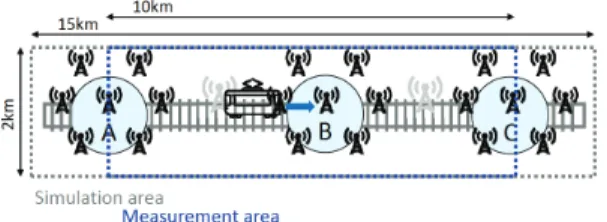
1) City setup: Figure 11 depicts the outline of the simula-tion and the parameters for city setup are described in Table II. Three train stations are located in the area and each train station is surrounded by seven static eNBs that have three sectors. These eNBs are located in hexagonal grids. One train, 200m long and 3m wide, goes from west (left) to east (right) at a constant 60km/h. This speed represents the average travel speed of commuter trains in the middle of metropolitan urban city. The simulation starts when the train is at the west edge,
Fig. 11. Simulation field.
TABLE II
SIMULATION PARAMETERS FOR CITY SETUP. Parameters Values Size of simulation area 2 km x 15 km Size of measurement area 2 km x 10 km
Number of base stations 21 (3 train station x 7 base stations) Number of sectors 3
Distance between train stations 5 km Train movement 60 km/h (constant)
and the measurement starts when the train is at station A, and ends when the train is at station C. The simulation ends when the train is at the east edge. A total of 500 non-train users are distributed in the coverage of each sector and those users do not move during simulation. Varied numbers of train users are uniformly distributed in the train. The eNB selection by users is based on received signal power, e.g., train users are likely to connect to the eNB from which a user device observes the strongest signal power.
We assume one extra base station, called additional BS, is added at each intermediate point between two train stations, i.e., (A and B) and (B and C). In order to evaluate the fundamental efficiency, we use five scenarios as follows.
[A] As a reference model, no additional BS.
[B-1] Additional BS without on/off switching or dynamic orientation functions.
[B-2] Additional BS with an on/off switching function but no dynamic orientation function.
[B-3] Additional BS with no on/off switching function but with a dynamic orientation function.
[B-4] Additional BS with both on/off switching and dy-namic orientation functions.
These scenarios are differentiated by the presence or absence of each function in order to simplify the determination of the performance benefit of each function.
2) Radio setup: The parameters for radio setup are de-scribed in Table III. We adopt the 800MHz frequency band for wireless communication, as is commonly used for LTE communication. To simplify the situation, user devices use only one channel in the simulation and the band width for the communication is 10MHz. The transmission power is 45dBm which means that the packet would be transferred for an approximately 2km distance, which is assumed be the size of macro-cell ordinarily deployed in cities. The path loss model is standardized in 3GPP [38] and fading would be modeled as a random process since it can be due to multi-path propagation, shadowing from obstacles, etc.. The multi-path
TABLE III
SIMULATION PARAMETERS FOR RADIO SETUP. Parameters Values Channel Frequency 800 MHz
LTE bandwidth 10MHz (50 RB / subframe) LTE Scheduler type ROUND-ROBIN eNB transmission power 45 dBm
Pathloss model COST231-Walfisch-Ikegami NLOS Shadowing model LOGNORMAL
Shadowing mean 10 dB
lossPLpxqis described as follows:
PLpxq P¯Lpxq Np0, σ2q, (10) ¯ PLpxq 55.9 38log10pxq p24.5 1.5 f 925qlog10pfq, (11)
where x is the distance from the base station and f is the frequency of the electromagnetic wave. The serving sector is simply decided by user devices seeking the highest gain, which means user devices handover as they connect to the base station that delivers the strongest signal. Dynamic switching of base stations when a train is closer/farther than the threshold from the base stations, with threshold for switching being the radio coverage of the base station. Dynamic orientation of the base station’s antennas to follow the movement of the trains. The angle and direction of the antenna are designed to face the middle of the train.
3) Application setup and evaluation metrics: In the sim-ulation, each user device connects to the network according to the connectivity models introduced in Section IV. After the simulation starts, a user u individually starts an active duration after a random waiting durationr0,paveragepCTq averagepITqq{2s. This draws1-st active durationdpau1qfor the active state from the CT/CNT model. After the active state ends, the user goes inactive and draws 1-st idle duration dpiu1q
from the IT/INT model. After the inactive state ends, the user goes active again, drawing a durationdpau2q from the CT/CNT model and again selecting a serving base station based on the received signal power. Each user repeats the above processes independently from each other, until the simulation ends.
To evaluate the typical performance metrics, we define the following applications and metrics. Each user device executes the applications while it is in the active state.
TCP-FTP.UseruPUcontinuously downloads files while
uis connected through a TCP session. In the beginning of each active duration, user device establishes a TCP session that lasts until the end of the active duration. Using the TCP-FTP application, we measure the mean throughputThU as follows. ThU 1 NU ¸ u 1 Tu n¸puq i1 dpaiuqthpiuq, (12) whereNU is the number of users, Tu is the total active
duration for useru,npuqis the number of active duration of useru,dpaiuqis thei-th active duration andthpiuqis the throughput for thei-th active duration of useru.
![Fig. 12. Relative performance normalized to [A].](https://thumb-us.123doks.com/thumbv2/123dok_us/507235.2559866/13.918.94.845.101.227/fig-relative-performance-normalized-to-a.webp)