Hussain, B., Du, Q., Imran, A. and Imran, M. A. (2019) Artificial intelligence-powered
mobile edge computing-based anomaly detection in cellular networks. IEEE
Transactions on Industrial Informatics, (doi:10.1109/TII.2019.2953201).
There may be differences between this version and the published version. You are
advised to consult the publisher’s version if you wish to cite from it.
http://eprints.gla.ac.uk/202352/
Deposited on: 5 November 2019
Enlighten – Research publications by members of the University of Glasgow
Artificial Intelligence-powered Mobile Edge
Computing-based Anomaly Detection in
Cellular Networks
Bilal Hussain,
Student Member, IEEE,
Qinghe Du,
Member, IEEE,
Ali Imran,
Member, IEEE,
and Muhammad Ali Imran,
Senior Member, IEEE
Abstract—Escalating cell outages and congestion—treated as
anomalies—cost a substantial revenue loss to the cellular opera-tors and severely affect subscriber quality of experience. State-of-the-art literature applies feed-forward deep neural network at core network (CN) for the detection of above problems in a single cell; however, the solution is impractical as it will overload the CN that monitors thousands of cells at a time. Inspired from mobile edge computing and breakthroughs of deep convolutional neural networks (CNNs) in computer vision research, we split the network into several 100-cell regions each monitored by an edge server; and propose a framework that pre-processes raw call detail records having user activities to create an image-like volume, fed to a CNN model. The framework outputs a multi-labeled vector identifying anomalous cell(s). Our results suggest that our solution can detect anomalies with up to 96% accuracy, and is scalable and expandable for industrial Internet of things environment.
Index Terms—Self-Organizing Networks, Self-Healing
Net-works, Call detail record, Deep learning, Convolutional Neural Networks, Big data analytics.
I. INTRODUCTION
D
RIVEN by ever increasing mobile data traffic, numberof connected mobile devices per capita [1], [2], and network capacity demand, current communication networks (4G) are becoming more complex and a quagmire to manage. It is indisputable that emerging wireless networks (5G) will be artificial intelligence (AI)-assisted and AI will play a crucial role in the management and orchestration of network resources [3]. Big Data [4] for AI algorithms are analogous to fuel for
an engine, and are generated at the core network (CN), cell,
and subscriber levels of a cellular network (delineated in [5]). Big Data analytics using advanced machine learning (subset of AI) algorithms is envisioned to be the key innovation and integral part of 6G communication ecosystem [6].
Network operators are facing challenges in reducing the operational expenditure (OPEX) while maintaining adequate
B. Hussain is with the School of Information and Communications En-gineering, Xi’an Jiaotong University, China; Shaanxi Smart Networks and Ubiquitous Access Research Center; and the Department of Electronic and Information Engineering, The Hong Kong Polytechnic University, Hong Kong (e-mail: [email protected]).
Q. Du is with the School of Information and Communications Engineering, Xi’an Jiaotong University, China, and is also with Shaanxi Smart Networks and Ubiquitous Access Research Center (e-mail: [email protected]). A. Imran is with the School of Electrical and Computer Engineering, University of Oklahoma, Tulsa, OK 74135 USA (e-mail: [email protected]). M. A. Imran is with the School of Engineering, University of Glasgow, Glasgow, G12 8QQ, U.K. (e-mail: [email protected]).
quality of service (QoS) for their subscribers. There are essentially two types of expenditures for the cellular network operators to bear: capital expenditure (CAPEX) which refers to acquisition and modernization of network entities, and oper-ational expenditure (OPEX) which refers to the amount spent on management and maintenance of the cellular network’s operations [7]. One of the major reasons for heightening OPEX and revenue loss is the escalation of network faults that result in outages. In fact, network maintenance and operation cost roughly one-fourth of the total revenue, out of which a significant portion is dedicated to cell outage—full, indicates a complete dysfunction of a cell and partial, means cellular service deterioration—management [7]. The faults and outages are likely to magnify in 5G networks due to the implemen-tation of small cells; making it arduous to manually manage the outages by heavily depending on the human experts, as is done in current cellular networks [7]. Network faults can occur due to hardware malfunctions, software problems, functional resource failures, loss due to overload situations, or communi-cation failures [8]. Self-healing is one of the four functions of self-organizing network (SON) [7] that can perform automatic detection of cellular outages and performance degradations, their root-cause analysis, and compensation of outage affected cells until the full recovery. It can play a decisive role in cutting down the OPEX by minimizing network outages and system downtime with least human intervention.
Besides outages, a cell can have an unusually high traffic demand at any time that could cause congestion if befit measures are delayed [9]: partial load offloading via neigh-boring base stations (BSs) [10] or enabling device-to-device (D2D) relay networks [11], [12], extra resource allocation [9], dynamic pricing especially in QoS-enabled networks [13], etc. The role of congestion detection becomes crucial during crowded events (sport matches, public demonstrations, vehicular traffic jams, etc.) having a surged traffic and capacity demand: network performance usually degrades due to a drastic change in population distribution, application workload and user behavior [14]. As a consequence, congestion occurs with denied user services (in the form of high connection timeouts and failures) due to scarce radio resources. Poor network performance can affect huge number of subscribers in such situations and can result in serious revenue loss in terms of increased churn rate. Hence, prompt detection of soared traffic and cell outage—both treated as anomalies in our paper and henceforth referred as so unless explicitly mentioned
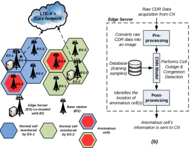
LTE-A’s Core Network Edge Server (ES) co-located with BS Base station (BS) Anomalous cells Normal cell monitored by ES-2 ES-2 ES-1 Normal cell monitored by ES-1 (a) BS-2 BS-3 BS-4 BS-2 BS-3 Pre-processing C N N M o d e l Post-processing Converts raw CDR data into an image Identifies the location of anomalous cell(s) Edge Server Raw CDR Data acquisition from CN Anomalous cell’s information is sent to CN Database (training samples) Performs Cell Outage & Congestion Detection (b) BS-1 BS-1 BS-4
Fig. 1. AI-powered MEC-based anomaly detection framework. (a)System model: call detail record (CDR) dataset is generated at the core network (CN) of a long term evolution-advanced (LTE-A) network. The cellular network is divided into two sub-grids (blue and green cell clusters), each having 4 base stations (BSs) and an edge server (ES 1 or ES 2) co-located with one of the BSs. Note, although we experiment using a sub-grid comprising 100 cells in this paper and a city can be divided into tens or even hundreds of such sub-grids, depending on the size of cells and city; in this figure for clarity, we only show two sub-grids each comprising 4 cells. For every subsequent time-interval (10-min), the CN shares raw CDRs of every cell in a sub-grid to its corresponding ES that processes them for anomaly detection. The ES then reports the cell ID of an anomalous cell (having a red inner hexagon) to CN for further curative actions.(b)The framework installed in the ES converts raw CDR data into a grid-image (pre-processing), deploys convolutional neural network (CNN) model to identify an anomalous cell(s) using the database (containing training samples) and forwards the information to the CN.
otherwise—is vital to avoid congestion, retain acceptable QoS, and recover a cell in time.
Past studies [7], [15] utilize various traditional machine learning techniques for cell outage detection (COD) ; however only [16] fully exploits more powerful technique known as deep learning (DL) [17], in which the authors utilize a feed-forward deep neural network (DNN) at the CN to detect anomalies in a single cell. A 5G network is anticipated to have40–50BSs/km2[18]; as an example, Milan, Italy (total
area of181.76km2) may require7,270−9,088BSsfor full
coverage. To detect anomalies for such a high number of BSs using this solution, the CN might computationally overload. Additionally, a major limitation of using a feed-forward DNN is the requirement of copious amount of resources: computa-tion power and storage; because, fundamentally each unit in a layer of the neural network is connected with each unit of the previous layer requiring huge amount of parameters to be processed and stored.
Inspired from the breakthroughs of deep convolutional neu-ral networks (CNNs) in computer vision research [19] and mobile edge computing (MEC), we propose a novel framework for anomaly detection that eases CN in terms of computational load and also consumes lesser computational resources as compared with the state-of-the-art DL-based cellular network anomaly detector [16]. We assume a peculiar cellular traffic pattern can well reflect the anomaly—unusually low user traf-fic activity indicates a cell outage or performance deterioration,
and unusually high traffic signals a potential congestion—and therefore, we utilize call detail records (CDRs) to detect the anomalies. Instead of processing the subscriber activities of all cells at CN, the computation-intensive tasks are distributed among different edge servers (ESs) (co-located with BSs) that target a subset of the total cells (see Fig. 1). Additionally, ESs perform data analytics using CDR dataset and are AI-powered: unlike the previous study in which quintessential (feed-forward) DNNs were utilized, we exploit the power of CNNs that are more efficient (discussed in Sec. IV-A). The information about identified anomalous cell(s) is then dispatched from ES to the CN for further remedial actions under self-healing (if cell outage occurred) or congestion-prevention mechanism (if soared user activity is detected). We can holistically relate our framework with MEC paradigm in which CN acts as cloud server (having centralized computation and processing from network’s perspective) and ES acts as a MEC server (offering decentralized architecture for storage, computation and connectivity) [20].
Following are the salient contributions of this study:
1. Employs a novel MEC-based framework to detect
anomalies in a grid of cells by exploiting real net-work CDR data and the power of CNNs.
2. Deploys a very deep CNN model called residual
network comprising 50 layers (ResNet-50) that yields additional performance as compared with a relatively simple model inspired from various classical CNN models, and analyzes both models in terms of per-formance and training time.
3. Detects surged user traffic activity that can act as an
early-warning against congestion in a cell, in addition to the anomalies pertaining to cell outages.
The rest of paper is organized as follows. Relevant work is summarized in Section II. Preliminaries to our proposed framework are explained in Section III. Framework’s imple-mentation is described in Section IV. Subsequently, results and framework’s performance evaluation are discussed in Sec-tion V. Finally, discussion on results, future insights including feasibility of our framework for industrial Internet of things (IIoT) environment and cloud radio access network (C-RAN) architecture, and concluding remarks are drawn in Section VI.
II. RELEVANTWORK
In this section, we discuss works related to COD focusing on utilizing DL technology and the works related to congestion detection. Readers can refer to [7] for an exhaustive literature survey on COD, in which the survey is divided to cover full and partial CODs, each focusing on works utilizing: Heuristic (solutions that utilize pre-defined rules dictated by the experts) and learning based (solutions based on machine learning) methodologies. In addition, Kline et al. [15] also discuss works related to COD in which machine learning techniques are utilized. However, both [15] and [7] lack works that have leveraged DL technology for COD.
Hussain et al. [16], [21] proposed a framework that utilizes feed-forward DNN to detect anomalies in a single cell of a cellular network. It pre-processes real CDRs to extract a 5-feature vector corresponding to user activities of a cell, that it
accepts as an input. The output is a binary number indicating 0 as normal and 1 as an anomaly. However, the solution is computationally expensive if applied to the whole network because of the reasons mentioned in the previous section. Masood et al. [22] presented a deep autoencoder (type of feed-forward DNN) based sleeping cell—a special case of a cell outage that occurs without triggering any alarm—detector that leverages minimization of drive test (MDT) measurement data generated by user equipments using a simulator. The data consist reference signal received power (RSRP) and signal to interference plus noise ratio (SINR) of neighboring and serving BSs. The model was trained on data obtained from normal operation with 7 macro cells and testing was done on data from outage scenario. Main issue with their approach, as also indicated in [7, Sec. IV C], is they only considered spatial data gathered for one time instance that results in instantaneous sleeping cell detection. Hence, the detected anomaly could be momentary, having little impact on QoS, and may vanish by the time it is compensated.
It is interesting to note that both, Hussain et al. [16] and Masood et al. [22] claimed their deep learning based approaches for anomaly detection eclipsed conventional ma-chine learning approaches: semi-supervised statistical-based detection [23] and one class support vector machine based detection, respectively. This is the rational behind our inclina-tion towards preferring deep learning models over tradiinclina-tional machine learning models.
Ramneek et al. [13] presented an analytical solution for congestion detection, as part of their paper, in QoS-enabled networks. The main idea is to monitor load on the network, by utilizing information extracted from the QoS-based scheduler, to determine the congestion level. Parwez et al. [9] proposed a technique using big-data (CDR) analytics and machine learning algorithms to identify region of interests (ROIs) as an anomaly that have unusually high user traffic activity. Since they analyzed CDRs of one week for the detection, their approach is impractical for systems that demand prompt de-tection. Overcoming this limitation and building upon the idea that such ROIs can have congestion if appropriate measures are delayed, Hussain et al. [23] proposed a semi-supervised machine learning algorithm to detect soared user traffic activity in past one hour CDR data of a cell, by analyzing its past user activity behavior. Cutting down detection cycle from one hour to 10 minutes and further enhancing the performance, the authors in their following work [16] proposed DL approach for the identification of such ROIs.
In contrast to all the above works, our approach is differ-ent as it provides a lighter solution for anomaly detection by utilizing deep CNNs instead of feed-forward DNNs and MEC-based architecture to divide computational load of CN among different ESs. Utilizing existing (CDR) data instead of requesting additional KPI-based data also makes our approach agile [23]. It detects both anomalies (outage and surged traffic activity that may lead to congestion) and in multiple cells at a time. Our approach also considers both, spatial and temporal dimensions leading to the detection of long-term outages instead of the instantaneous ones.
ITALY Trento 2970 1 117 11350 11466 3087 3096 3204 3213 Trento 3330 3447 3564 3681 3798 3915 3321 3555 3672 3789 3906 3438 2979 4023 4032 Milan
Fig. 2. Spatial description of our dataset: It is spread over a 117×98 (Trentino) grid, located in northern Italy.(Top-left)The grid is overlaid with Italy’s map using its GPS coordinates.(Top-right)The grid is zoomed-in for clarity. Our dataset contains user-activities of a total number of 6259 cells, highlighted by the larger blue region. We chose10×10sub-grid for our experiments, shown in red; while to proof scalability of our method, we chose 15×15sub-grid, shown in inner light-blue region.(Bottom)The sub-grid is zoomed-in for clarity. It consists of 100 cells, each having a side length of 1 km.
III. PRELIMINARIES
A. System Model and Description of the Dataset
The system model is shown in Fig. 1(a). It is based on long term evolution - advanced (LTE-A) mobile network ar-chitecture (described in [9, Fig. 1]). The CDR dataset utilized in this study was generated at LTE-A’s CN and made public by Telecom Italia as part of their big data challenge [24]. The main idea is to divide a network into regions called sub-grids, each consisting 100 cells and an edge server (ES) co-located with one of the BSs. The ES is equipped with our proposed anomaly detection framework that mainly handles preprocessing and comprises a deep CNN model. For every subsequent 10-min duration: 1) the ES acquires raw CDR data of each cell in its sub-grid from the CN; 2) the framework pre-processes the data to construct a grid-image that is acceptable as an input by the deep CNN model; 3) the model trains on a dataset (available in the attached database) containing past user behavior of the cells and detects anomalous cell(s) in the current example; 4) finally the ES passes information of the faulty cell(s) to the CN that further takes curative actions (mentioned in Sec. I). The process is shown in Fig. 1(b).
The data are geo-referenced and designed in spatio-temporal manner; they contain over 171.4 million logs for 6259 cells
spread over a 117×98 grid (known as Trentino grid) in
Trentino province, Italy [24]. Each cell has a side length of approx. 1km. We have mapped the spatial locations of the grid and cells according to their GPS coordinates, delineated in
Fig. 2. The dataset is temporally split into 10-min timestamps for a 62-days duration (comprising of a single file for each day) from 1/11/2013 to 1/1/2014. On average, 2.76 million logs per file are present and each log contains the following user activity values: call incoming, SMS incoming, call outgoing, SMS outgoing and Internet usage. Some subscriber-related details—such as, location, phone number, and exact unit (or number) of activity—are excluded for privacy preservation. However, the available amount of activities is proportionate to the real quantity of activities [23]. Sample of similar raw CDRs can be observed in [9, Fig. 2].
B. Data Preprocessing and Synthesis
CNN processes grid-like data such as a time-series or an image [25, Ch. 9]. In preprocessing stage, we convert raw
CDRs into a 10×10×5 3D matrix x(i) ∈ Rn [0] H×n [0] W×n [0] C
henceforth referred as “grid-image”, where i is the index,
n[0]H is the height, n[0]W is the width, and n[0]C is the number
of channels of the grid-image. The height and width make up 100 entries representing cells chosen from the bottom portion of the Trentino grid, illustrated as red squares in Fig. 2. The channels comprise 5 feature (subscriber activity) values of the selected cells: Call incoming, SMS incoming, call outgoing, SMS outgoing, and Internet usage. Hence, each pixel of the grid-image contains the above activity values of a corresponding cell, recorded during a 10-min duration. In order to excavate meaningful pattern in the dataset, an avalanche of examples each representing past instances are required; however, only 62 instances are available in the current dataset for each time-resolution. To remedy this, we combine timestamps for a 3-hour duration and generate 1,116
grid-images (6 timestamps per hour × 3 hours × 62 days),
represented as a 4D matrixXtotal∈Rm×n
[0] H×n [0] W×n [0] C, where
m is the total number of grid-images.
Since we are dealing with supervised learning and have
unlabeled data, we generate labels Ytotal ∈ Rm×100 on the
basis of euclidean distance, where 100 represents the total number of output classes (each denoting a cell). An output class indicating 1 means an anomaly and the corresponding cell is faulty, and 0 means the corresponding cell’s operation
is normal. For each output class, we mark 1 if kµ−σk2 >
kak2>kµ+σk2, wherea∈R5represents the corresponding
cell’s activity. The elements of mean µ ∈ R5 and standard
deviation σ ∈R5 can be calculated using standard textbook
equations [23, Eq. 1, 2].
C. Shuffling and Splitting the Data
The order of Xtotal and Ytotal is synchronously shuffled
to make the algorithm more effective since it is using mini-batches (a subset of the entire dataset). The mini-mini-batches en-able the optimization algorithm (mini-batch gradient descent) to rapidly compute approximate gradient estimates instead of computing exact gradient, making the algorithm converge faster [25, Ch. 8]. The shuffled dataset is then split into training and test sets according to a ratio of 7:3, each comprising 781 and 335 grid-images with labels, respectively.
D. Performance Metrics
For the performance evaluation of our framework, we utilized the following common metrics of machine learning literature: precision, recall, accuracy, error rate, false positive
rate (FPR), and F1. Readers can refer [23] for a contextual
explanation of these metrics. E. Software
MATLAB was exploited for preprocessing, GPS mapping, and results generation. Keras [26] was also utilized to actu-alize the CNN models. Experimentation was performed in a commercial PC (i7-7700T CPU, 16GB RAM, and Windows 10 64-bit operating system) with an in-built GPU (NVIDIA GeForce 930MX).
IV. IMPLEMENTATION OFANOMALYDETECTOR
In this section, we describe generic architecture of the CNN followed by a discussion on how it fits in with our research, the architecture’s utility in building a relatively simple deep CNN model and lastly, we describe the ResNet-50 model. A. CNN’s Generic Architecture
CNN [25, Ch. 9] has the following three fundamental layers, as can also be found in Fig. 3(a):
1) Convolution layer: accepts an input volume (or
acti-vations of previous layer) A[l−1] ∈
Rm×n [l−1] H ×n [l−1] W ×n [l−1] C ,
where l represents number of the current layer; and filters
F[l] ∈ Rf
[l]×f[l]×n[l−1]
C ×n
[l]
C, where f[l] is the filter size,
f[l]×f[l]×n[l−1]
C is the dimension of a single filter andn
[l]
C is the total number of filters. The convolution layer performs parallel convolution operations between input volume and each filter, adds bias, applies a rectified linear unit (ReLU) [25, Sec. 6.3] function and lastly, stack up each result to form an output
A[l] ∈Rm×n [l] H×n [l] W×n [l] C. The height n[l]
H can be calculated as:
n[Hl]=bn
[l−1]
H + 2p
[l]−f[l]
s[l] + 1c (1)
where, p[l] is the number of padding and s[l] is the stride.
Padding is a technique to add zeros around the border of the input image to prevent the height and width from shrinking, as output dimension reduces due to convolution operation. Stride is the distance between successive utilization of filter
on the input volume. Formula for width n[Wl] can be written
by replacingn[Hl−1] withn[Wl−1] in Eq. 1.
2) Pooling layer: improves computational efficiency,
re-duces requirement for storing parameters and adds robustness to some of the detected features [25, Sec. 9.3]. Max function is commonly utilized in pooling layers that pools maximum numbers from regions of input volume (and from each channel,
independently) depending on the filter size f, to generate
the output volume. If the dimension of input volume is
nH×nW×nC, the dimension of output volume can be derived
using Eq. 1 withp= 0asbnH−f
s + 1c × b
nW−f
s + 1c ×nC .
As an example, we considerM axP ool1layer, illustrated in
Fig. 4(a). The pooling layer accepts an input volume having
10 X 10 X 5 14 X 14 X 5 13 X 13 X 8 Zero Padding p = 2 Conv1 2 X 2, 8 (i.e. f = 2, 8 filters) s = 1 5000 1000 100 FC2 Binary cross entropy loss function Input Volume Output Z e ro P a d d in g C o n v BN Re L U M a x P o o l C o n v M o d u le ID M o d u le x 2 C o n v M o d u le ID M o d u le x 3 C o n v M o d u le ID M o d u le x 5 C o n v M o d u le ID M o d u le x 2 F la tt e n F C 1 0 0
Phase 1 Phase 2 Phase 3 Phase 4 Phase 5
Output 10 X 10 X 5 p = 5 (Binary cross entropy loss function) (b) Input Volume f = 3 s = 2 7x7, 64 s = 2 (a) C o n v BN Re L U C o n v BN Re L U C o n v BN Re L U C o n v BN Conv Module a[l] a[l+3] 1x1, F3 Stride s 3 x 3, F2 p is “same” 1x1, F3 Skip connections Main paths (c) C o n v BN Re L U C o n v BN Re L U C o n v BN Re L U a[l] a[l+3] 1x1, F1 3 x 3, F2 p is “same” 1x1, F3 ID Module 1x1, F1 Stride s MaxPool1 f = 2 s = 2 6 X 6 X 8 Conv2 2 X 2, 16 (i.e. f = 2, 16 filters) s = 1 5 X 5 X 16 MaxPool2 f = 2 s = 2 2 X 2 X 16 Conv3 1 X 1, 32 (i.e. f = 1, 32 filters) s = 1 2 X 2 X 32 MaxPool3 f = 2 s = 2 1 X 1 X 32 Flatten 32 FC1 20x20x5 7x7x64 3x3x64 3x3x64 3x3x64 3x3x64 3x3x256 3x3x256 3x3x256 3x3x256 3x3x256 3x3x256 3x3x64 3x3x64
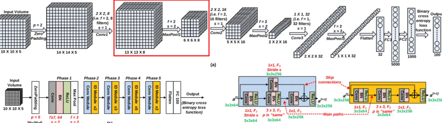
Fig. 3. CNN models.(a)The simple CNN model accepts an input volume having features’ values of100cells.Conv1−Conv3represents convolution layers, each executing convolution operation, batch normalization and ReLU activation function.M axP ool1−M axP ool3 represents the pooling layers utilizing a max function.F C1andF C2are fully connected layers. The output is a multi-label classifier having100classes, each representing a corresponding cell of the sub-grid in Fig. 2(bottom). Output dimension of the convolution and pooling layers are computed using Eq. 1. Note, the input volume consists of a single example (grid-image) for clarity. Readers can refer to Sec. IV. A. 2 for the working ofM axP ool1layer, highlighted as red rectangle.(b)The residual network model with 50 layers accepts the input volume. AfterZeroP adding, the information flows through different phases.P hase1consists of a convolution layer, followed by batch normalization (BN) and ReLU activation functions, and a (Max) pooling layer.P hase2−P hase5stacks the two residual modules in a linear fashion. After flattening the output of last phase, we implement a fully connected layer and finally the output layer.(c)The residual modules, convolutional (Conv) and identity (ID), are shown along with the skip connections and the main paths for the flow of information. Each module consists of three hidden layers. The number of filters used in the layers [F1,F2 andF3] of each module are listed in Table I. Note, the output dimensions shown in green are designated for phase 2 only.
13 X 13 X 8 MaxPool1 f = 2 s = 2 6 X 6 X 8 (2, 2) window 3 3 2 1 0 3 2 1 0 6 5 9 5 6 5 9 5 7 9 1 2 7 9 1 2 9 9 2 4 7 5 2 4 7 5 7 s=2 ……. ……. …. …. .…. 13 X 13 6 X 6 (a) (b)
Fig. 4. Operation of a Max-Pooling Layer
dimension—the height and width is calculated by using Eq. 1.
The layer utilizes following hyperparameters: filter sizef = 2
and stride s= 2. This combination of hyperparameter values
is common and it shrinks the input’s size by a factor of 2. For simplicity, we demonstrate the max pooling operation in a single channel, illustrated in Fig. 4(b). The layer slides a
(f, f) window over input and stores the maximum value of the window in the output. It performs the same operation for each channel and finally stacks the results to form the output volume.
3) Fully connected layer: functions like the hidden layer of
a feed-forward neural network (described thoroughly in [16]), in which each hidden unit is connected to all hidden units of the previous layer.
B. Why Choose CNN?
Parameter sharing and sparse interactions [25, Sec. 9.2] are the main reasons for CNN’s popularity and dramatic increase
in computational efficiency as compared with feed-forward neural networks; because these result in lesser parameters to compute and store. For example, consider a convolution layer
Conv1 in Fig. 3(a) having an input volume of dimensions
14×14×5, a filter size f = 2, and 8 number of filters.
Using Eq. 1 with p= 0 and aforementioned values, we can
calculate the dimension of output volume: 13×13×8. The
total number of parameters utilized in this (single convolution
layer) operation is 40: 2∗2(for one filter) +1(for bias) = 5
parameters per filter and40parameters for8filters. However,
if this was a feed-forward neural network, the input would be
980 units (flatten version of the input volume:14∗14∗5), the
output would be 1352 units (13∗13∗8), and the total number
of required parameters would be 1.32 million (980∗1352).
CNN is hence faster and require lesser resources (computation and storage). Due to the mentioned benefits and the fact that we are dealing with grid-like data (of 100 cells), CNN is our natural choice.
C. Simple CNN Model
Many models available today have put together the building blocks in different settings (in terms of number of layers and the approach of connecting them together) to form a CNN. LeNet-5 [27], AlexNet [28] and VGG [29] are some of the classical CNN models; while ResNet [30] and Inception-v4 [31] represent some modern ones (readers can refer to [26, Sec. Applications] for an exhaustive list of modern CNN models). Our first approach, illustrated in Fig. 3(a), is inspired from works of the aforementioned classical models, in which we utilize the building blocks in addition to batch normalization (thoroughly explained in the next paragraph) to detect
anoma-lies. Our model accepts a10×10×5grid-image as an input.
It then pads zero along the edges (zero-padding) with p= 2
layers (Conv1, M axP ool1, Conv2, M axP ool2, Conv3,
M axP ool3). The dimension of output volume of each layer can be computed by utilizing Eq. 1. The resultant volume is finally flattened and passed through two fully connected layers
(F C1 and F C2). Finally, we utilize binary cross entropy
loss function for a multi-labeled output as each class is not mutually exclusive.
Batch normalization (BN) [32] is a powerful technique of adaptive re-parametrization, used to accelerate training process and make DNN more robust. Training a DNN leads to a problem of covariance shift: distribution of earlier layers’ parameters shifts, that affects the later layer’s capability to adopt accordingly and results in a slow training process. Instead of just normalizing the input features values of the network, the technique normalizes the activations of each hidden layer. It makes the deeper layers’ parameters more robust to changes, to earlier layers’ parameters; hence, en-hancing the network’s stability [25, Sec. 8.7], [32]. Readers can refer to [33] for more detailed analysis on BN. We apply BN after the convolution operation and before utilizing the activation function. Therefore in Fig. 3(a), each convolution layer incorporates BN in addition to convolution operation and ReLU activation.
D. Residual Network Model
To enhance the performance of our framework, we utilized residual network comprising 50 layers (ResNet-50), as shown in Fig. 3(b). Depth of a neural network plays a crucial role in accurately representing more complex functions and in raising the overall network’s performance [29]. However, deeper net-works are harder to train as they suffer from gradient vanishing and exploding problems [25] that hinder with the convergence of the network, making it unbearably slow. Deeper networks also suffer from a degradation problem: as we add more layers the accuracy saturates and then quickly reduces, leading to an elevated training error [30].
Residual network [30] effectively deals with these problems by stacking residual modules on top of one another, shown as P hase 2−5 in Fig. 3(b). We first elaborate functioning of a residual module used in the residual networks by using ID module of Fig. 3(c). In the figure, the information flows
from input a[l] to the output activation a[l+3] through two
unique paths. The downward path, called main path, has three parts. The information first goes via initial part consisting three blocks having a convolution layer, BN, and a non-linear activation function, respectively; governed by the following standard equations:
z[l+1]=W[l+1]a[l]+b[l+1] (2)
a[l+1]=g(z[l+1]) (3)
where,W[l+1]is the weight matrix,b[l]is the bias vector,g(.)
is the non-linear activation function,a[l]is the input, anda[l+1]
is the output of the initial part. The BN is utilized throughout the model to boost up the training.
Similarly, the blocks in the third part are governed by the following equations (ignoring the other path and a summation operation):
z[l+3]=W[l+3]a[l+2]+b[l+3] (4)
a[l+3]=g(z[l+3]) (5)
In residual networks, a[l] is fast-forwarded to a deeper
hidden layer in the neural network where it is summed up with the output of that layer before applying a non-linear activation function. This is known as a skip connection, as shown in the figure. Hence, Eq. 5 will be altered as follows:
a[l+3]=g(z[l+3]+a[l]) (6)
The addition of a[l] makes it a residual module and this
enables the activations of one layer to skip some layers and be directly fed to a deeper layer. This also allows a gradient (during back-propagation) to be directly back-propagated to an earlier layer. Here, we are assuming that the dimensions
of both, inputa[l] andz[l+3] (and therefore outputa[l+3]) are
same in order to perform the summation. This kind of residual module is known as identity (ID) module.
If the dimensions of input (a[l]) and output activations
(a[l+3]) mismatch then a convolution layer in the skip
con-nection is introduced to adjust the input a[l] to a different
dimension, so that the dimensions match up in the final sum-mation. This type of residual module is called Convolutional (Conv) module, illustrated in the Fig. 3(c)(left).
Moreover, we can now analyze the residual network archi-tecture with 50 layers depicted in Fig. 3(b). As an example, we
can concentrate on the parts starting from the input toP hase2
of the architecture. In the following, we will discuss in term of dimensions so that the purpose of ID and Conv modules can be explained subsequently; and Eq. 1 is extensively utilized in computing the output dimensions of various layers. The
input grid-image having dimension10×10×5is zero-padded
with paddingp= 5to have an output volume with dimension
20 ×20 ×5. It is then passed to P hase1 comprising a
convolution layer with filter sizef = 7, total number of filters
nC = 64, and strides= 2; that transforms the dimension to
7×7×64. Lastly, Max Pool havingf = 3ands= 2generates
the output volume with dimension3×3×64.
For P hase2, let’s focus on Fig. 3 (c)(left) having Conv
module that will have an input dimension of3×3×64from
the earlier layer. The main path contains 3 parts. The initial
part has convolution layer having f = 1,nC =F1= 64(see
Table I), ands= 1. It yields volume with identical dimensions
as of the input’s. The convolution layer in the second part also results output with same dimension as of the input’s because it is utilizing “same” convolution (in which padding is set so that the output’s dimension remains same as of the input’s). The
third part having a convolution layer withf = 1,nC =F3=
256(see Table I), ands= 1will convert the input’s dimension
from 3×3×64 to 3×3×256. Finally, convolution layer
in the skip connection, that has input volume of dimension
3×3×64, scales up the input’s dimension to3×3×256 by
utilizing the parameter values: f = 1, nC =F3 = 256(see
Table I), ands= 1. The outputs from both convolution layers
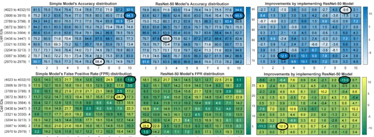
Fig. 5. Performance distributions. Accuracy (blue) and false positive rate (FPR) (green) distributions of our simple CNN (left) and ResNet-50 (middle) models are displayed in the heatmaps. The best and worst performance values are marked in black annotations. The right heatmaps display improvements we got for each cell by implementing ResNet-50 model instead of the simple model (negative values indicate degradation in the relevant performance metric). The annotations in right heatmaps represent maximum improvements and degradations. Note, each item in a heatmap corresponds to the cell of the sub-grid in Fig. 2(bottom). The models were executed for 200 epochs.
TABLE I
HYPERPARAMETERS USED IN OURRESNET-50MODEL
Phase Number of filters used in thelayers [F
1,F2,F3] of each module Stride s
2 [64, 64, 256] 1
3 [128, 128, 512] 2
4 [256, 256, 1024] 2
5 [512, 512, 2048] 2
main path) can be added as they are now compatible: have the same dimensions.
The ID modules of P hase2have similar function as of the
aforementioned Conv module, with the exception of the skip connection’s design that does not has any layer in it. This is because the input of the ID modules has same dimension as of
the output of convolution layer in it’s third part:3×3×256;
hence, convolution layer is not needed in the skip connection. The hyperparameter values used in our model can be found in Fig. 3(b) and (c) (in red annotations), and Table I.
V. EXPERIMENTALRESULTS ANDPERFORMANCE
EVALUATION
We demonstrate performances of our simple CNN and ResNet-50 models in Fig. 5 using the test set. The figure
shows 10×10 heatmaps: blue ones representing accuracy
distributions and the green ones representing false positive rate (FPR) distributions; with the left, middle and right ones pertaining to the simple model, ResNet-50 model and improve-ments we achieved by implementing ResNet-50 over simple model, respectively. Each position in a heatmap relates to a corresponding cell of the sub-grid in Fig. 2(bottom). The best and worst performance values in the left and middle heatmaps are marked in black annotations, while the annotations in right heatmaps represent maximum improvements and degradations. As we can observe in the figure that the performance results pertaining to different cells vary; this is because fundamentally each cell has it’s own unique distribution of user activity
values in terms of call incoming, SMS incoming, call outgoing, SMS outgoing, and Internet usage, from which our framework creates grid-images. The model learns different underlying distributions and hence the performance result for each cell is different.
The accuracy of cell 2976 (row 1, column 7)—the worst performing cell—using the simple model is significantly im-proved from 68.4% to 75.5% by using ResNet-50 model. Cell 3915 (9, 10) yielded maximum accuracy 94.3% using simple CNN, and is slightly further improved to 95.5% using ResNet-50 model. Additionally, the maximum and minimum FPRs using the simple model are 24.7% and 1.8% for cell 3680 (7, 9) and 4032 (10, 10), respectively; they are further reduced to 17.7% and 1.1%, respectively, when ResNet-50 is utilized. The minimum FPR in ResNet-50’s distribution is 1% for cell
2970 (1, 1), a 3× reduction from 3.2% when simple model
was utilized.
However, performance also degrades for some cells, as evident in the right-hand heatmaps (indicated with negative values). For example, observe accuracy of cell 3440 (5, 3) that worsened from 71.9% using simple model to 69.6% using ResNet-50 model. Similarly, ResNet-50 model resulted in higher FPR of 28.8% for cell 3087 (2, 1), a significant increase as compared with 17.5% when simple model is used. Based on the above observations, the individual cell’s performance can either be ameliorated or degraded by us-ing ResNet-50 model; however, the overall performance of ResNet-50 model improves as compared with its counterpart, as evident in Table II. Also note the training time for
ResNet-50 model is about 7×higher than of the simple model.
To proof scalability of our proposed method, we scaled-up
the size of our grid-image from10×10×5 to15×15×5,
to include a total number of225 grids. For this purpose, we
selected cell IDs starting from5076to6728, depicted as inner
light-blue square grid in Fig. 2 (top-right), and kept rest of the parameters of each model same as before. Table III conveys the overall test performance and training time of both models, and
TABLE II
COMPARISON OF OVERALL TEST PERFORMANCE AND TRAINING TIME OF THE TWO MODELS FOR ANOMALY DETECTION
Metric Simple CNN Model ResNet-50 Model Improvement Accuracy 78.99% 81.06% 2.07% Error Rate 21% 18.94% 2.06% Precision 69.99% 73.59% 3.6% Recall 64.59% 67.21% 2.62% FPR 13.81% 12.03% 1.78% F1 67.18% 70.26% 3.08%
Training Time 3.52 min 25.58 min -TABLE III
COMPARISON OF OVERALL TEST PERFORMANCE AND TRAINING TIME OF THE TWO MODELS FOR ANOMALY DETECTION WHEN15×15×5
DIMENSION GRID-IMAGE IS UTILIZED
Metric Simple CNN Model ResNet-50 Model Improvement Accuracy 78.21% 80.4% 2.19% Error Rate 21.78% 19.59% 2.19% Precision 64.42% 72.5% 8.08% Recall 61.9% 56.34% -FPR 14.74% 9.21% 5.53% F1 63.13% 63.41% 0.28%
Training Time 3.88 min 26.34 min
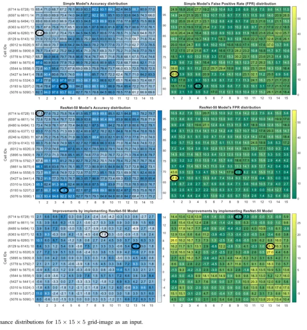
-the improvements achieved by leveraging ResNet-50 model over simple CNN model. Fig. 6 demonstrates performance (accuracy and FPR) distributions of both models for each of
the chosen cell IDs in the form of top and middle 15×15
heatmaps. The bottom heatmaps represent the improvements. Similar to our observations of Fig. 5, we can also observe in Fig. 6 that the performance of some cells has improved and for some cells, it has deteriorated by applying ResNet-50 model. We can also observe that the overall accuracy and error rate values in Table III resemble their counterparts in Table II. Additionally, similar to the trend we previously observed in Table II, ResNet-50 model in our current experiments has also achieved better performance results as compared with the simple CNN model except for the recall. Hence, our proposed method is scalable.
If we compare Table III with Table II, it is interesting to observe that overall training time do not proportionally increase as we increase the resolution of input image. Hence, the resolution can be enhanced to accommodate anomaly detection for a larger number of cells with the expense of slightly higher computation time. This is because of the two properties of CNN discussed in Sec. IV-B—which enable the number of parameters in a layer of CNN to remain constant even if the input’s resolution is varied.
Finally, we compare our model’s performance with the performance of feed-forward DNN proposed in Hussain et al. [21]. Hence for comparison, we adopt their feed-forward DNN model with the same hyper-parameter values and implement
it on the 100 cells depicted in Fig. 2 (red grid). Due to the
space constraint, we only show the test accuracy distribution in Fig. 7, which can be compared with our simple CNN model’s accuracy distribution in Fig. 5. In addition, comparison of overall test accuracy and training time of our simple CNN and ResNet-50 models with feed forward DNN model is shown in Fig. 8. Although we can find some instances of cells having
feed forward DNN outperformed other models in Fig. 7, but overall the DNN model performed poorly. As evident in Fig. 8, DNN yielded worst overall test accuracy as well as training time as compared with both of our models.
VI. CONCLUSION ANDINSIGHTS FOR FUTURE WORK
We found our AI-powered mobile edge computing (MEC)-based anomaly detection framework (installed in an edge server (ES), co-located with a base station) can efficiently detect anomalous cell(s) in a 100-cell region with 70% - 96% accuracy, depending on an individual cell’s characteristics. Our method is computationally light as compared with state-of-the-art solution [16]: it eases computational load on the core network (CN) by leveraging MEC approach and convolutional neural network (CNN)—that we found to be efficient in terms of utilizing fewer parameters than feed-forward deep neural network (DNN), as explained and demonstrated in Sec. IV-A. We further investigated two CNN models: sim-ple model (inspired from the traditional CNN models) and ResNet-50 model (adopted from a recent paper on residual learning [30]). We found the latter yielded superior overall performance than the formal but consumes a significantly large training time—creating a trade off between training time and performance.
Since our framework is designed to detect anomalies within minutes—the conventional techniques involve subscriber com-plaints and drive tests that consume hours and sometimes days to detect the anomaly (cell outage) [34]—this potentially improves QoS and truncates OPEX as timely identification of anomalous cell means quicker problem resolution. Detection of surged traffic activity in a region can also act as an early-warning towards potential congestion that might choke the network. This enhances user quality of experience as timely identification of such situation will help avoid user dissatisfaction. The addition of Internet activity feature that was missing in most of the previous studies [9], [23], makes our framework robust as it can detect situation such as musical concert that might have slightly increased SMS/call activities considered as normal but escalated Internet traffic (as people frequently use social media to share their moments).
In the current (hardware and parametric) settings, the simple CNN model seems more appropriate for online learning envi-ronment as it can detect anomalies within the arrival of next timestamp (10-min) unless we utilize more advanced hardware for timely anomaly detection using ResNet-50 model. Perhaps, with a more powerful quantum processing hardware [35] in near-future, the emerging and future cellular networks can even train much deeper and advanced neural network models (ResNet-152 [30], Inception-v4 [31], etc.), faster and within lesser time for more enhanced performance. Another limitation to our research’s practical implementation is the requirement of ground-truth labels that can be overcome by assigning labels with the help of fault data having archived alarms’ logs [5]. Selecting optimum hyperparameters values can also ameliorate performance. Hyperparameter tuning is essentially an optimization loop that reruns the machine learning model with various configurations of hyperparameter values in a
Fig. 6. Performance distributions for15×15×5grid-image as an input.
Fig. 7. Feed-forward DNN model’s accuracy distribution.
search space (having ranges for all the hyperparameters) to yield minimum error. This can be done manually by relying on humans having domain knowledge or as mentioned above, it can be a grid search having a discretized hyperparameter search space. However, this is a computationally expensive process. In this connection, random search algorithm [36] is comparatively more efficient and can be utilized in our future work.
(a) (b)
Fig. 8. Performance compassion of our simple CNN and ResNet-50 models with feed-forward DNN model proposed in [21]. Purple bars indicate best result among all.
For the practical settings, since we can categorize the cellular network with our proposed MEC-based approach as an MEC system with heterogeneous servers, the decision to choose the number of cells monitored by an edge server can depend on multifaceted reasons which mainly concerns resource management [20, Sec. III. C.]. For example,
deter-mining whether to offload computation to an ES or if the core network has sufficient computation power at a given instance to perform all the calculations (server selection problem [20, Sec. III. C.], [37]); for the case where the computations are offloaded to an ES, determining how much calculations an ES can handle and then performing pre-processing and subsequently allocating number of cells accordingly; etc.
We speculate our framework can also conform to the cloud radio access network (C-RAN) architecture, where there are massive number (hundreds or even thousands) of remote radio heads (RRHs) controlled by a centralized, collaborative and cloud-based baseband unit (BBU) pool [38]. In our research context, a BBU pool can act as an ES monitoring user activities pertaining to several RRHs; however, this direction needs further investigation. In industrial Internet of things, our work can also be extended to address anomaly (fault due to device malfunction, connectivity failures, delayed communication, etc.) detection in which a middleware (fog) connected with various entities (actuators, robots, machines, sensors, etc.) monitors their data to report anomalies [39]–[41]. Fog com-puting is utilized in the industry for local comcom-puting to address delay and security concerns, and a fog node can perform tasks similar to the ones performed by the ES in our research.
In conclusion, the paper presents a robust, scalable, and novel framework based on MEC, powered by deep CNN (computationally efficient than feed-forward DNN utilized in the latest research) and fueled by real CDR (spatio-temporal) dataset to detect anomalies (pertaining to cell outage and performance degradations, and surged cellular traffic activity leading to a potential congestion) in a 100-cell sub-grid; relieving CN from tremendous computational load of doing data analytics for each cell in the network.
ACKNOWLEDGMENT
The research reported in this paper was supported in part by the National Natural Science Foundation of China under the Grant No. 61671371 and the Fundamental Research Funds for the Central Universities.
REFERENCES
[1] Cisco, “Cisco Visual Networking Index: Global Mobile Data Traffic Forecast Update, 2016-2021,”White Paper, Feb. 2017.
[2] Q. Du, H. Song, and X. Zhu, “Social-Feature Enabled Communications among Devices towards Smart IoT Community,”IEEE Commun. Mag., vol. 57, no. 1, pp. 130-137, Jan. 2019.
[3] R. Liet al., “Intelligent 5G: When Cellular Networks Meet Artificial Intelligence,”IEEE Wireless Commun., vol. 24, no. 5, pp. 175-183, Oct. 2017.
[4] C. Wu, E. Zapevalova, Y. Chen, and F. Li, “Time Optimization of Multiple Knowledge Transfers in the Big Data Environment,” Tech
Science Press, vol. 54, no.3, pp.269-285, 2018.
[5] A. Imran, A. Zoha, and A. Abu-Dayya, “Challenges in 5G: how to empower SON with big data for enabling 5G,”IEEE Netw., vol. 28, no. 6, pp. 27-33, Nov.-Dec. 2014.
[6] K. David, and H. Berndt, “6G Vision and Requirements: Is There Any Need for Beyond 5G?,”IEEE Veh. Technol. Mag., vol. 13, no. 3, pp. 72-80, Sep. 2018.
[7] A. Asghar, H. Farooq, and A. Imran, “Self-Healing in Emerging Cel-lular Networks: Review, Challenges, and Research Directions,”IEEE
Commun. Surveys Tut., vol. 20, no. 3, pp. 1682-1709, 3rd Quart., 2018.
[8] 3GPP,Telecommunication Management; Fault Management; Part 1: 3G
Fault Management Requirements,3GPP Standard TS 32.111-1-V13.0.0,
2016.
[9] M. S. Parwez, D. Rawat, and M. Garuba, “Big data analytics for user-activity analysis and user-anomaly detection in mobile wireless network,”IEEE Trans. Ind. Informat., vol. 13, no. 4, pp. 2058-2065, Aug. 2017.
[10] Y. Li, B. Shen, J. Zhang, X. Gan, J. Wang, and X. Wang, “Offloading in HCNs: Congestion-aware network selection and user incentive design,”
IEEE Trans. Wireless Commun., vol. 16, no.10, pp. 6479-6492, Oct.
2017.
[11] H. Zhang, Z. Wang, Q. Du, “Social-Aware D2D Relay Networks for Stability Enhancement: An Optimal Stopping Approach,”IEEE Trans.
Veh. Technol., vol. 67, no. 9, pp. 8860-8874, Sep. 2018.
[12] Z. Liao, J. Liang, and C. Feng, “Mobile relay deployment in multihop relay networks,”Computer Communications, vol. 112, pp. 14-21, 2017. [13] Ramneek, P. Hosein, W. Choi, and W. Seok, “Congestion detection for QoS-enabled wireless networks and its potential applications,” J.
Commun. Netw., vol. 18, no. 3, pp. 513-522, June 2016.
[14] M. Z. Shafiqet al., “A first look at cellular network performance during crowded events,” inProc. ACM Sigmetrics, 2013, pp. 17-28.
[15] P. V. Klaine, M. A. Imran, O. Onireti, and R. D. Souza, “A Survey of Machine Learning Techniques Applied to Self-Organizing Cellular Networks,”IEEE Commun. Surveys Tut., vol. 19, no. 4, pp. 2392-2431, 4th Quart., 2017.
[16] B. Hussain, Q. Du, and P. Ren, “Deep Learning-Based Big Data-Assisted Anomaly Detection in Cellular Networks,” inProc. IEEE Glob.
Commun. Conf. (GLOBECOM), 2018, pp. 1-6.
[17] Z. Liao, R. Zhang, S. He, D. Zeng, J. Wang, and H. Kim, “Deep Learning-Based Data Storage for Low Latency in Data Center Net-works,”IEEE Access, vol. 7, pp. 26411-26417, 2019.
[18] X. Ge, S. Tu, G. Mao, C. Wang, and T. Han, “5G Ultra-Dense Cellular Networks,” IEEE Wireless Commun., vol. 23, no. 1, pp. 72-79, Feb. 2016.
[19] Y. LeCun, Y. Bengio, and G. Hinton, “Deep Leering,”Nature, vol. 521, no. 7553, pp. 436–444, May 2015.
[20] Y. Mao, C. You, J. Zhang, K. Huang, and K. B. Letaief, “A Survey on Mobile Edge Computing: The Communication Perspective,” IEEE
Commun. Surveys Tut., vol. 19, no. 4, pp. 2322-2358, 4th Quart., 2017.
[21] B. Hussain, Q. Du, S. Zhang, A. Imran, and M. A. Imran, “Mobile Edge Computing-Based Data Driven Deep Learning Framework for Anomaly Detection,” inIEEE Access, vol. 7, pp. 137656-137667, Sep. 2019. [22] U. Masood, A. Asghary, A. Imrany, and A. N. Mian, “Deep Learning
Based Detection of Sleeping Cells in Next Generation Cellular Net-works,” inProc. IEEE Glob. Commun. Conf. (GLOBECOM), 2018, pp. 206-212.
[23] B. Hussain, Q. Du, and P. Ren, “Semi-Supervised Learning Based Big Data-Driven Anomaly Detection in Mobile Wireless Networks,”China
Commun., vol. 15, no. 4, pp. 41-57, Apr. 2018.
[24] [Online] https://dandelion.eu/datagems/SpazioDati/trentino-grid/ description/
[25] I. Goodfellow, Y. Bengio, and A. Courville,Deep learning, Cambridge, MA, USA: MIT Press, 2016.
[26] [Online] https://keras.io/
[27] Y. LeCun, L. Bottou, Y. Bengio, and P. Haffner, “Gradient-Based Learning Applied to Document Recognition,”Proc. IEEE, vol. 86, no. 11, pp. 2278-2324, Nov. 1998.
[28] A. Krizhevsky, I. Sutskever, and G. E. Hinton, “ImageNet Classification with Deep Convolutional Neural Networks,”Advances Neural Inform.
Process. Syst. (NIPS), 2012, pp. 1097-1105.
[29] K. Simonyan, and A. Zisserman, “Very deep convolutional networks for large-scale image recognition,” Proc. Int. Conf. Learning
Representa-tions (ICLR), 2015.
[30] K. He, X. Zhang, S. Ren, and J. Sun, “Deep Residual Learning for Image Recognition,” arXiv:1512.03385 [cs.CV], Dec. 2015.
[31] C. Szegedy, S. Ioffe, V. Vanhoucke, and A. A. Alemi, “Inception-v4, Inception-ResNet and the Impact of Residual Connections on Learning,”
Proc. 31st AAAI Conf. Artificial Intelligence (AAAI-17), 2017, pp.
4278-4284.
[32] S. Ioffe, and C. Szegedy, “Batch Normalization: Accelerating Deep Net-work Training by Reducing Internal Covariate Shift,” arXiv:1502.03167 [cs.LG], Mar. 2015.
[33] Y. Cai, Q. Li, and Z. Shen, “A Quantitative Analysis of the Effect of Batch Normalization on Gradient Descent,” Proc. 36th Int. Conf.
Machine Learning, 2019, pp. 882-890.
[34] A. Zoha, A. Saeed, A. Imran, M. A. Imran, and A. Abu-Dayya, “Data-driven analytics for automated cell outage detection in self-organizing networks,” in Proc. 11th Int. Conf. Des. Reliable Commun. Netw.
[35] F. Tacchino, C. Macchiavello, D. Gerace, and D. Bajoni, “An Artificial Neuron Implemented on an Actual Quantum Processor,” arXiv:1811.02266 [quant-ph], Nov. 2018.
[36] J. Bergstra, and Y. Bengio, “Random Search for Hyper-Parameter Optimization,”J. Mach. Learn. Res., vol. 13, no. 1, pp. 281-305, Jan. 2012.
[37] Z. Liao, J. Wang, S. Zhang, J. Cao, and G. Min, ”Minimizing Move-ment for Target Coverage and Network Connectivity in Mobile Sensor Networks,” in IEEE Transactions on Parallel and Distributed Systems, vol. 26, no. 7, pp. 1971-1983, 1 July 2015.
[38] M. Peng, Y. Sun, X. Li, Z. Mao, and C. Wang, “Recent Advances in Cloud Radio Access Networks: System Architectures, Key Techniques, and Open Issues,” IEEE Commun. Surveys Tut., vol. 18, no. 3, pp. 2282–2308, 3rd Quart., 2016.
[39] M. Aazam, S. Zeadally, and K. A. Harras, “Deploying Fog Computing in Industrial Internet of Things and Industry 4.0,”IEEE Trans. Ind.
Informat., vol. 14, no. 10, pp. 4674-4682, Oct. 2018.
[40] A. Al-Fuqaha, M. Guizani, M. Mohammadi, M. Aledhari, and M. Ayyash, “Internet of Things: A Survey on Enabling Technologies, Pro-tocols, and Applications,”IEEE Communications Surveys & Tutorials, vol. 17, no. 4, pp. 2347-2376, Fourthquarter 2015.
[41] A. Gharaibeh et al., “Smart Cities: A Survey on Data Management, Security, and Enabling Technologies,” IEEE Communications Surveys
& Tutorials, vol. 19, no. 4, pp. 2456-2501, Fourthquarter 2017.
Bilal Hussain [S’10] received B.E. degree (First-class honours) in electrical engineering from Bahria University, Pakistan in 2010 and M.Sc. degree in information and communications engineering from University of Leicester, U.K. in 2011. He is cur-rently pursuing his Ph.D. degrees in information and communications engineering from Xi’an Jiaotong University, China and The Hong Kong Polytechnic University, Hong Kong (under a dual Ph.D. degree program).
His broader research interests include applications of artificial intelligence and big data analytics in wireless communication systems (6G/5G mobile networks), mobile edge and fog computing, and cyber-physical systems security.
Qinghe Du [S’09-M’12] received his B.S. and
M.S. degrees both from Xi’an Jiaotong University, China, and his Ph.D. degree from Texas A&M University, USA. He is currently a Professor of Information and Communications Engineering De-partment, Xi’an Jiaotong University, China. His re-search interests include mobile wireless communi-cations and networking with emphasis on statisti-cal QoS provisioning, secure wireless transmissions, 5G networks, D2D/M2M networks, cognitive radio networks, mobile multicast, etc. He has published over 100 technical papers. He received the Best Paper Award in IEEE GLOBECOM 2007. He serves and has served as an Associate Editor of IEEE COMMUNICATIONS LETTERS and an Editor of KSII TRANSACTIONS ON INTERNET AND INFORMATION SYSTEMS. He serves and has served as a Technical Program Co-Chair for IEEE ICCC Workshop on Internet of Things (IoT) 2013, 2014, and 2015, a Track Co-Chair for IIKI 2015, and the Publicity Co-Chairs for IEEE ICC 2015 Workshop on IoT/CPS-Security, IEEE GLOBECOM 2011, ICST WICON 2011, and ICST QShine 2010. He also serves and has served as the Technical Program Committee Members for many world-renowned conferences including IEEE INFOCOM, GLOBECOM, ICC, PIMRC, VTC, etc.
Ali Imran is founding director of AI4Networks
Research Lab (www.ai4networks.com) at the
Uni-versity of Oklahoma where he is leading several multinational and industry lead projects on AI for wireless networks. He is also co-founder of a start-up AISON (www.aison.co). Dr Imran’s research on AI enabled wireless networks has played pioneering role in this emerging area and has been supported by $4M in nationally and internationally competitive re-search funding and recognised by several prestigious awards such as IEEE Green ICT YP award 2017, VPR Outstanding International Impact Award at the University of Oklahoma, 2017 and best paper award IEEE CAMAD 2013. He has published over 100 refereed journal and conference papers and has several patents granted and pending. In 2018 he has been named William H. Barkow Presidential Professor at the University of Oklahoma.
He is routinely invited to serve as an advisor to key stakeholder in cellular network eco-system and as a speaker and a panellist on international industrial fora and academic conferences on this topic. Before joining OU in Jan 2014, for three years he has worked as a Research Scientist at QMIC, Qatar. Between Oct-2007 and Oct-2011, he has worked in the Institute of Communications Systems (5GIC) University of Surrey, UK. In that position, he has contributed to a number of pan-European and international research projects while working in close collaboration with key industrial players. He is an Associate Fellow of Higher Education Academy (AFHEA), UK; president of ComSoc Tulsa Chapter; Senior Member IEEE, Member of Advisory Board for Special Technical Community on Big Data at IEEE Computer Society, and board member of ITERA. For more detailed Dr. Imran see: www.ali-imran.org
Muhammad Ali Imran [M’03–SM’12] received
the M.Sc. (Distinction) and Ph.D. degrees from Imperial College London, London, U.K., in 2002 and 2007, respectively. He is the Vice Dean Glasgow College UESTC and Professor of communication systems with the School of Engineering, University of Glasgow. He is an Affiliate Professor at the University of Oklahoma, Norman, OK, USA, and a visiting Professor with the 5G Innovation Centre, University of Surrey, Guildford, U.K. He has more than 20 years of combined academic and industry experience, working primarily in the research areas of cellular communication systems. He has 15 patents, has authored or co-authored more than 400 journals and conference publications, and has been principal or coprincipal investigator on more than 10 million in sponsored research grants and contracts. He has supervised more than 40 successful Ph.D. graduates. He was the recipient of the award of excellence in recognition of his academic achievements, conferred by the President of Pakistan, the IEEE ComSocs Fred Ellersick Award 2014, FEPS Learning and Teaching Award 2014, and Sentinel of Science Award 2016. He was twice nominated for Tony Jeans Inspirational Teaching Award. He is a shortlisted finalist for The Wharton-QS Stars Awards 2014, QS Stars Reimagine Education Award 2016 for innovative teaching, and VCs Learning and Teaching Award in University of Surrey. He is a Fellow of IET and a senior fellow of Higher Education Academy (SFHEA), U.K.