STRUCTURAL NONPARAMETRIC COINTEGRATING REGRESSION
By
Qiying Wang and Peter C. B. Phillips
May 2008
COWLES FOUNDATION DISCUSSION PAPER NO. 1657
COWLES FOUNDATION FOR RESEARCH IN ECONOMICS
YALE UNIVERSITY
Box 208281
New Haven, Connecticut 06520-8281
http://cowles.econ.yale.edu/
Structural Nonparametric Cointegrating Regression
∗
Qiying Wang
School of Mathematics and Statistics
The University of Sydney
Peter C. B. Phillips
Cowles Foundation, Yale University
University of Auckland & Singapore Management University
February 13, 2008
Abstract
Nonparametric estimation of a structural cointegrating regression model is stud-ied. As in the standard linear cointegrating regression model, the regressor and the dependent variable are jointly dependent and contemporaneously correlated. In nonparametric estimation problems, joint dependence is known to be a major com-plication that affects identification, induces bias in conventional kernel estimates, and frequently leads to ill-posed inverse problems. In functional cointegrating re-gressions where the regressor is an integrated time series, it is shown here that inverse and ill-posed inverse problems do not arise. Remarkably, nonparametric ker-nel estimation of a structural nonparametric cointegrating regression is consistent and the limit distribution theory is mixed normal, giving simple useable asymp-totics in practical work. The results provide a convenient basis for inference in structural nonparametric regression with nonstationary time series. The methods may be applied to a wide range of empirical models where functional estimation of cointegrating relations is required.
Key words and phrases: Brownian Local time, Cointegration, Functional regression, Gaus-sian process, Integrated process, Kernel estimate, Nonlinear functional, Nonparametric regression, Structural estimation, Unit root.
JEL Classification: C14, C22.
∗Wang acknowledges partial research support from Australian Research Council. Phillips acknowl-edges partial research support from a Kelly Fellowship and the NSF under Grant No. SES 06-47086.
1
Introduction
A good deal of recent attention in econometrics has focused on functional estimation in structural econometric models and the inverse problems to which they frequently give rise. A leading example is a structural nonlinear regression where the functional form is the object of primary interest. In such systems, identification and estimation are typically much more challenging than in linear systems because they involve the inversion of integral operator equations which may be ill-posed in the sense that the solutions may not exist, may not be unique and may not be continuous. Some recent contributions to this field include Newey, Powell and Vella (1999), Newey and Powell (2003), Ai and Chen (2003), Florens (2003), and Hall and Horowitz (2004). Overviews of the ill-posed inverse literature are given in Florens (2003) and Carrasco, Florens and Renault (2006). All of this literature has focused on microeconometric and stationary time series settings.
In linear structural systems problems of inversion from the reduced form are much simpler and conditions for identification and consistent estimation techniques have been extensively studied. Under linearity, it is also well known that the presence of nonsta-tionary regressors can provide a simplification. In particular, for cointegrated systems involving time series with unit roots, structural relations are actually present in the re-duced form (and therefore always identified) because of the unit roots in a subset of the determining equations. In fact, such models can always be written in error correction or reduced rank regression format where the structural relations are immediately evident.
The present paper shows that nonstationarity leads to major simplifications in the context of structural nonlinear functional regression. The primary simplification arises because in nonlinear models with endogenous nonstationary regressors there is no ill-posed inverse problem. In fact, there is no inverse problem at all in the functional treatment of such systems. Furthermore, identification does not require the existence of instru-mental variables that are orthogonal to the equation errors. Finally, and perhaps most importantly for practical work, consistent estimation may be accomplished using standard kernel regression techniques, and inference may be conducted in the usual way and is valid asymptotically under simple regularity conditions. These results for kernel regression in structural nonlinear models of cointegration open up many new possibilities for empirical research.
The reason why there is no inverse problem in structural nonlinear nonstationary systems can be explained heuristically as follows. In a nonparametric structural setting
it is conventional to impose on the disturbances a zero conditional mean condition given certain instruments, in order to assist in identifying an infinite dimensional function. Such conditions lead to an integral equation involving the conditional probability distribution of the regressors and the structural function integrated over the space of the regressor. This equation describes the relation between the structure and reduced form and its solution, if it exists and is unique, delivers the unknown structural function. But when the endogenous regressor is nonstationary there is no invariant probability distribution of the regressor, only the local time density of the limiting stochastic process corresponding to a standardized version of the regressor as it sojourns in the neighborhood of a particular spatial value. Accordingly, there is no integral equation relating the structure to the reduced form. In fact, the structural equation itself is locally also a reduced form equation in the neighborhood of this spatial value. For when an endogenous regressor is in the locality of a specific value, the systematic part of the structural equation depends on that specific value and the equation is effectively a reduced form. In fact, the random wandering nature of stochastically nonstationary time series ensures that the regressor inevitably departs from any particular locality and thereby assists in tracing out (and identifying) the structural function. The process is similar to the manner in which instruments may shift the location in which a structural function is observed and in doing so assist in the process of identification when the data are stationary.
Linear cointegrating systems reveal a strong form of this property. As mentioned above, in linear cointegration the inverse problem disappears completely because the structural relations continue to be present in the reduced form. Indeed, they are the same as reduced form equations up to simple time shifts, which are of no importance in long run relations. In nonlinear structural cointegration, the same behavior applies locally in the vicinity of a particular spatial value, thereby giving local identification of the structural function and facilitating estimation.
In linear cointegration, the signal strength of a nonstationary regressor ensures that least squares estimation is consistent, although the estimates are well-known to have second order bias (Phillips and Durlauf, 1986; Stock, 1987) and are therefore seldom used in practical work. Much attention has therefore been given in the time series literature to the development of econometric estimation methods that remove the second order bias and are asymptotically and semiparametrically efficient.
regression methods are consistent and that under some regularity conditions they are also asymptotically mixed normally distributed, so that conventional approaches to inference are possible. These results constitute a major simplification in the functional treatment of nonlinear cointegrated systems and they directly open up empirical applications with existing methods.
The paper is organized as follows. Section 2 introduces the model and assumptions. Section 3 provides the main result on the consistency and limit distribution of the kernel estimator in a structural model of nonlinear cointegration. Section 4 reports a simulation experiment exploring the finite sample performance of the kernel estimator. Section 5 concludes and outlines ways in which the present paper may be extended. Proofs and various subsidiary technical results are given in Sections 6 and 7 as Appendices to the paper.
2
Model and Assumptions
We consider the following nonlinear structural model of cointegration
yt=f(xt) +ut, t = 1,2, ..., n, (2.1)
whereutis a zero mean stationary error,xtis a jointly dependent nonstationary regressor, and f is an unknown function to be estimated with the observed data {yt, xt}nt=1. The conventional kernel estimate off(x) in model (2.1) is given by
ˆ f(x) = Pn t=1ytKh(xt−x) Pn t=1Kh(xt−x) , (2.2)
whereKh(s) = h1K(s/h),K(x) is a nonnegative real function, and the bandwidth param-eter h≡hn →0 as n→ ∞.
The limit behavior of ˆf(x) has been investigated in past work in some special situ-ations, notably where the error process ut is a martingale difference sequence and there is no contemporaneous correlation between xt and ut. These are strong conditions, they are particularly restrictive in relation to the conventional linear cointegrating regression framework, and they are unlikely to be satisfied in econometric applications. However, they do facilitate the development of a limit theory by various methods. In particular, Karlsen, Myklebust and Tjøstheim (2007, KMT) investigated ˆf(x) in the situation where
xt is a recurrent Markov chain; and Wang and Phillips (2006, WP) considered an al-ternative treatment by making use of local time limit theory and, instead of recurrent
Markov chains, worked with partial sum representations of the type xt =Ptj=1ξj where
ξj is a general linear process. These authors showed that the limit theory for ˆf(x) has links to traditional nonparametric asymptotics for stationary models even though the rates of convergence are different and typically slower whenxt is nonstationary. However, the strong conditions under which the asymptotic theory of KMT and WP is developed limits its usefulness in applications. It seems particularly important to relax conditions of independence, so that the system is a structural model that allows joint dependence between the regressor and dependent variable in the regression. The goal of the present paper is to remove this assumption of independence and to develop a limit theory for structural functional estimation in the context of nonstationary time series.
Throughout the paper we let {t}t≥1 be a sequence of independent and identically
distributed (iid) continuous random variables withE1 = 0,E21 = 1 and for which 1 has
a densityd(x). The sequence{t}t≥1 is assumed to be independent of another iidrandom
sequence {λt}t≥1. We use the following assumptions in the asymptotic development.
Assumption 1. xt = Pt j=1ηj where ηj = P∞ k=0φkj−k with φ ≡ P∞ k=0φk 6= 0 and P∞ k=0k2|φk|<∞.
Assumption 2. ut =u(t, t−1, ..., t−m0, λt) satisfies Eut = 0 and Eu4t <∞ for t ≥m0,
where u(x0, x1, ..., xm0, y) is a real measurable function on Rm0+2. We define ut = 0 for 1≤t≤m0−1.
Assumption 3. K(x) is a nonnegative bounded three times continuous differentiable function satisfying R K(x)dx <∞and R |K(i)(x)|dx <∞ for i= 1,2,3.
Assumption 4. For given x, there exists a real function f1(s, x)such that, when h
suffi-ciently small, |f(hy+x)−f(x)| ≤h f1(y, x)for all y∈R and
R∞
−∞K(s)f1(s, x)ds < ∞.
Assumption 1 is standard in a cointegrating regression framework, so that xt is a partial sum of linear process innovations that satisfy a simple summability condition with long run moving average coefficient φ 6= 0. Assumption 2 allows the equation error ut to be serially dependent and cross correlated with xs for |t−s| < m0, thereby inducing
endogeneity in the regressor. In the asymptotic development below, m0 is assumed to be
finite but this could likely be relaxed under some additional conditions and with greater complexity in the proofs, although that is not done here. It is not necessary for ut to depend on λt, in which case there is only a single innovation sequence. However, in most practical cases involving cointegration between two variables, we can expect that there
will be two innovation sequences.
Assumption 3 places stronger conditions on the kernel function than is usual in kernel estimation, requiring integrable derivatives to the third order. These conditions are needed for technical reasons in the proofs and they are clearly satisfied for many commonly used kernels. Assumptions 4, which was used in WP, is quite weak and can be verified for various kernels K(x) and regression functions f(x). For instance, if K(x) is a standard normal kernel or has a compact support, a wide range of regression functions f(x) are included. Thus, commonly occuring functions like f(x) = |x|α and f(x) = 1/(1 +|x|α) for some α >0 satisfy Assumption 4.
3
Main result and outline of the proof
The limit theory for the conventional kernel regression estimate ˆf(x) turns out to be very simple and is given in the following theorem.
THEOREM 3.1. For any h satisfying nh2 → ∞ and nh6 →0,
h n X t=1 Kh(xt−x) 1/2 ( ˆf(x)−f(x)) →D N(0, σ2), (3.1) where σ2 = E(u2 m0) R∞ −∞K 2(s)ds R∞ −∞K(x)dx . Remarks
(a) The proof of (3.1) is given in the Appendix. To outline the essentials of the argument here we split the error of estimation ˆf(x)−f(x) as
ˆ f(x)−f(x) = Pn t=1utKh(xt−x) Pn t=1Kh(xt−x) + Pn t=1 f(xt)−f(x) Kh(xt−x) Pn t=1Kh(xt−x) .
It is readily seen that
h n X t=1 Kh(xt−x) 1/2 ( ˆf(x)−f(x)) = n X t=1 utZnt + Θ1n/Θ2n, (3.2) where Znt = K xth−x /Θ2n with Θ22n= Pn t=1K xt−x h and Θ1n = n X t=1 f(xt)−f(x) K xt−x h .
It has been proved in WP that Θ1n/Θ2n →P 0, which requires that the “signal” Θ2
2n→ ∞, in Probab., which in turn requires that nh2 → ∞. The stated result will then follow if we prove
n (nh2)−1/4 [nt] X k=1 ukK[(xk−x)/h], (nh2)−1/2 n X k=1 K[(xk−x)/h] o →D c0N L1/2(t,0), d0L(1,0) , (3.3) on D[0,1]2, where c20 = φ E(um02 ) R−∞∞ K2(s)dt, d0 = φ R∞ −∞K(s)ds, L(t,0) is the
local time process at the origin of a Brownian motion{W(t)}t≥0, andN is a standard
normal variate independent of L(t,0). The local time process L(t, a) is defined by
L(t, a) = lim →0 1 2 Z t 0 I{|W(r)−a| ≤}dr. (3.4)
Indeed, since P(L(1,0) > 0) = 1, the required result (3.1) follows by (3.3) and the continuous mapping theorem. It remains to prove (3.3), which is done in the Appendix. In fact, it is clearly sufficient for the required result to show that the finite dimensional distributions converge in (3.3).
(b) Result (3.1) shows that ˆf(x) is consistent and has an asymptotic distribution that is mixed normal even in the presence of an endogenous regressor. The mixing variate in the limit distribution depends on the local time process L(1,0), as follows from (3.3). In finite samples, the performance of the functional estimation procedure will depend on how much time the processxtspends around the pointxand how well the bandwidth concentrates attention on this point. As remarked earlier, consistency depends on h → 0, so that function estimation is localized at a single point x as
n→ ∞. The conditionsnh2 → ∞ and nh6 →0 in the theorem require thath tend
to zero faster than n−1/6 but not as fast as n−1/2.
(c) The bandwidth choice h turns out to be particularly important in structural func-tional estimation when there is contemporaneous correlation betweenxtandut. For when h is fixed as n → ∞ the estimate ˆf(x) can be shown to be asymptotically biased and when h tends to zero slowly this bias is manifest even in very large samples. Some illustrative simulations are reported in the next section.
4
Simulations
This section reports the results of a simulation experiment investigating the finite sam-ple performance of the kernel regression estimator. The generating mechanism follows (2.1)and has the form
yt = f(xt) +ut, ∆xt=t,
ut = (λt+θt)/ 1 +θ2
1/2 ,
where (t, λt) are iid N(0, σ2I2). The following two regression functions were used in the
simulations: fA(x) = ∞ X j=1 (−1)j+1sin (jπx) j2 , fB(x) =x 3 .
The first function corresponds (up to a scale factor) to the function used in Hall and Horowitz (2005) and is truncated at j = 4 for computation. Figs. 1 and 2 graph these functions (the solid lines) and the mean simulated kernel estimates (broken lines) over the intervals [0,1] and [−1,1] for kernel estimates of fA and fB, respectively. Bias, variance and mean squared error for the estimates were computed on the grid of values
{x= 0.01k:k = 0,1, ...,100} for [0,1] and {x=−1 + 0.02k;k= 0,1, ...,100} for [−1,1] based on 10,000 replications. Simulations were performed for θ = 1 (weak endogeneity) and θ = 100 (strong endogeneity), with σ = 0.1, and for the sample size n = 500. A Gaussian kernel was used with bandwidths h=n−10/18, n−1/2, n−1/3, n−1/5.
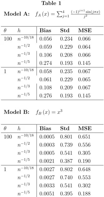
Table 1 shows the performance of the regression estimate ˆf computed over various bandwidths, h, and endogeneity parameters, θ, for the two models. In both models the degree of endogeneity (θ) in the regressor has a negligible effect on the properties of the kernel regression estimate when h is small. It is also clear that estimation bias can be substantial, particularly for model A with bandwidth h = n−1/5, corresponding to
the conventional rate for stationary series. Bias is substantially reduced for the smaller bandwidths h = n−1/2, n−1/3 at the cost of some increase in dispersion and is further
reduced when h = n−10/18 although this choice and h = n−1/2 violate the condition
nh2 → ∞ of theorem 3.1. The downward bias in the case of ˆfA over the domain [0,1] appears to be due to the periodic nature of the function fA and the effects of smoothing over x values for which the function is negative. The bias in ˆfB is similarly towards the origin over the whole domain [−1,1]. The performance characteristics seem to be little
affected by the magnitude of the endogeneity parameter θ. For model A, finite sample performance in terms of MSE seems to be optimized for h close to n−1/2. For model B,
h = n−1/5 delivers the best MSE performance largely because of the substantial gains
in variance reduction with the larger bandwidth that occur in this case. Thus, bias reduction through choice of a very small bandwidth may be important in overall finite sample performance for some regression functions but much less so for other functions. Of course, if h→0 so fast thatnh2 6→ ∞then the “signal” Pn
t=1K
xt−x
h
6→ ∞and the kernel estimate is not consistent.
Table 1 Model A: fA(x) = P4 j=1 (−1)j+1sin(jπx) j2 θ h Bias Std MSE 100 n−10/18 0.056 0.234 0.066 n−1/2 0.059 0.229 0.064 n−1/3 0.106 0.208 0.066 n−1/5 0.274 0.193 0.145 1 n−10/18 0.058 0.235 0.067 n−1/2 0.061 0.229 0.065 n−1/3 0.108 0.209 0.067 n−1/5 0.276 0.193 0.145 Model B: fB(x) =x3 θ h Bias Std MSE 100 n−10/18 0.0005 0.801 0.651 n−1/2 0.0003 0.739 0.556 n−1/3 0.0005 0.541 0.305 n−1/5 0.0021 0.387 0.190 1 n−10/18 0.0027 0.802 0.648 n−1/2 0.0027 0.740 0.553 n−1/3 0.0033 0.541 0.302 n−1/5 0.0051 0.395 0.188
Figs. 1 and 2 show results for the Monte Carlo approximations to EfˆA(x)
and
EfˆB(x)
corresponding to bandwidthsh=n−1/2 (broken line),h=n−1/3 (dotted line),
approximations toEfˆA(x)
andEfˆB(x)
together with a 95% pointwise “estimation band”. As in Hall and Horowitz (2005), these bands connect points f(xj ±δj) where each δj is chosen so that the interval [f(xj)−δj, f(xj) +δj] contains 95% of the 10,000 simulated values of ˆf(xj) for models A and B, respectively. Apparently, the bands are quite wide, reflecting the much slower rate of convergence of the kernel estimate ˆf(x) in the nonstationary case. In particular, since xt spends only
√
n of its time in the neighborhood of any specific point, the effective sample size for pointwise estimation purposes is√500 ∼22.Whenh=n−1/3,it follows from theorem 3.1 that the convergence rate is (nh2)1/4 =n1/12, which is far slower than the rate (nh)1/2
=n2/5 for conventional
kernel regression.
5
Conclusion
The two main results in the present paper have important implications for applications. First, there is no inverse problem in structural models of nonlinear cointegration of the form (2.1) where the regressor is an endogenously generated integrated process. This result reveals a major simplification in structural nonparametric regression in cointegrat-ing models, avoidcointegrat-ing the need for instrumentation and completely eliminatcointegrat-ing ill-posed functional equation inversions. Second, functional estimation of (2.1) is straightforward in practice and may be accomplished by standard kernel methods. These methods yield consistent estimates that have a mixed normal limit distribution, thereby validating con-ventional methods of inference in the nonstationary nonparametric setting.
The results open up some new possibilities for functional regression in empirical re-search with integrated processes. In addition to many possible empirical applications with the methods, there are some interesting extensions of the ideas presented here to other useful models involving nonlinear functions of integrated processes. In particular, additive nonlinear cointegration models and partial linear cointegration models may be treated in a similar way to (2.1). There are also issues of specification testing, functional form tests, and cointegration tests, which may now be addressed using the methods of the paper. We plan to report on some of these extensions in later work.
6
Proof of Theorem 3.1
As shown in Remark (a), the proof of the theorem essentially amounts to proving (3.3). To do so, we will make use of various subsidiary results which are proved here and in the next section.
First, it is convenient to introduce the following definitions and notation. If α(1)n ,
α(2)n ,...,α(nk)(1≤n ≤ ∞) are random elements ofD[0,1], we will understand the condition
(α(1)n , α(2)n , ..., α(nk))→D (α(1)∞, α(2)∞, ..., α(∞k))
to mean that for all α(1)∞, α(2)∞,..., α∞(k)-continuity sets A1, A2,...,Ak
P α(1)n ∈A1, α(2)n ∈A1, ..., α(nk) ∈Ak
→P α(1)∞ ∈A1, α(2)∞ ∈A2, ..., α(∞k) ∈Ak
.
[see Billingsley (1968, Theorem 3.1) or Hall (1977)]. D[0,1]k will be used to denote
D[0,1]×...×D[0,1], thek-times coordinate product space of D[0,1]. We still use ⇒ to denote weak convergence on D[0,1].
In order to prove (3.3), we use the following lemma.
LEMMA 6.1. Suppose that{Ft}t≥0 is an increasing sequence ofσ-fields,q(t)is a process
that isFt-measurable for eacht and continuous with probability 1,Eq2(t)<∞andq(0) = 0. Letψ(t), t≥0,be a process that is nondecreasing and continuous with probability 1 and satisfiesψ(0) = 0andEψ2(t)<∞. Letξbe a random variable which isF
t-measurable for
each t ≥0. If, for any γj ≥0, j = 1,2, ..., r, and any 0≤s < t≤t0 < t1 < ... < tr<∞,
E e−Prj=1γj[ψ(tj)−ψ(tj−1)]q(t)−q(s)| F s = 0, a.s., Ee−Prj=1γj[ψ(tj)−ψ(tj−1)][q(t)−q(s)]2−[ψ(t)−ψ(s)] | F s = 0, a.s.
then the finite-dimensional distributions of the process (q(t), ξ)t≥0 coincide with those of
the process(W[ψ(t)], ξ)t≥0, where W(s) is a standard Brownian motion withEW2(s) =s
independent of ψ(t).
Proof. This lemma is an extension of Theorem 3.1 of Borodin and Ibragimov (1995, page 14) and the proof follows from the same lines as in their work. Indeed, by using the fact that ξ is Ft-measurable for each t ≥0, it follows from the same arguments as in the proof of Theorem 3.1 of Borodin and Ibragimov (1995) that, for any t0 < t1, ..., tr < ∞,
αj ∈R and s∈R, EeiPrj=1αj[q(tj)−q(tj−1)]+isξ =EheiPrj−=11αj[q(tj)−q(tj−1)]+isξE eiαr[q(tr)−q(tr−1)] | F tr−1 i =Ehe−α 2 r 2 [ψ(tr)−ψ(tr−1)]ei Pr−1 j=1αj[q(tj)−q(tj−1)]+isξ i =...=Ee−α 2 r 2 Pr j=1[ψ(tj)−ψ(tj−1)]+isξ,
which yields the stated result. 2
By virtue of Lemma 6.1, we now obtain the proof of (3.3). Technical details of some subsidiary results that are used in this proof are given in the next section. Set
ξn = 1 d0 √ nh2 n X k=1 K[(xk−x)/h], ζn(t) = 1 √ n [nt] X k=1 k, ζn0(t) = 1 √ nφ [nt] X k=1 ηk, Sn(t) = 1 c0(nh2)1/4 [nt] X k=1 ukK[(xk−x)/h], ψn(t) = 1 d1 √ nh2 [nt] X k=1 u2kK2[(xk−x)/h],
for 0≤t≤1, where c0 and d0 are defined as in (3.3), andd1 =φ Eu2m0
R∞
−∞K 2(s)dt.
We will prove in Propositions 7.1 and 7.2 thatζn0(t)⇒W0(t),ξn →D ψ(1) andψn(t)⇒
ψ(t) on D[0,1], where ψ(t) := L(t,0) and L(t, s) is a local time process of the Wiener process {W0(t),0 ≤ t ≤ 1} defined by (3.4). Furthermore we will prove in Proposition 7.4 that {Sn(t)}n≥1 is tight on D[0,1]. These facts imply that {Sn(t), ψn(t), ζn0(t), ξn}n≥1
is tight on D[0,1]4. Hence, for each {n0} ⊆ {n}, there exists a subsequence {n00} ⊆ {n0}
such that
Sn00(t), ψn00(t), ζ0
n00(t), ξn00 →dη(t), ψ(t), W0(t), ψ(1) ,
onD[0,1]4, whereη(t) is a process continuous with probability one by noting (7.19) below.
By virtue of (7.1), we also have
Sn00(t), ψn00(t), ζn00(t), ξn00 →dη(t), ψ(t), W0(t), ψ(1) , (6.1)
on D[0,1]4. Write F
s =σ{W0(t),0 ≤t ≤1;η(t),0≤ t ≤s}. It is readily seen that Fs ↑ andη(s) isFs-measurable for each 0≤s ≤1. Also note thatψ(t) (for any fixedt∈[0,1]) is Fs-measurable for each 0≤s≤1. If we prove that for any 0≤s < t≤1,
Eη(t)−η(s)| Fs = 0, a.s., (6.2) E[η(t)−η(s)]2−[ψ(t)−ψ(s)] | Fs = 0, a.s., (6.3)
then it follows from Lemma 6.1 that the finite-dimensional distributions of (η(t), ξ) co-incide with those of {N L1/2(t,0), L(1,0)}, where N is normal variate independent of
L(t,0). The result (3.3) therefore follows, sinceη(t) does not depend on the choice of the subsequence.
Let 0 ≤ t0 < t2 < ... < tr = 1, r be an arbitrary integer and G(...) be an arbitrary bounded measurable function. In order to prove (6.2) and (6.3), it suffices to show that
E[η(tj)−η(tj−1)]G[η(t0), ..., η(tj−1);W0(t0), ..., W0(tr)] = 0, (6.4)
E[η(tj)−η(tj−1)]2−[ψ(tj)−ψ(tj−1)] G[η(t0), ..., η(tj−1);W0(t0), ..., W0(tr)] = 0.(6.5)
Recall (6.1). Without loss of generality, we assume the sequence{n00}is the{n}itself. Since Sn(t), Sn2(t) and ψn(t) for each 0 ≤t ≤1 are uniformly integrable (see Proposition 7.3), the statements (6.4) and (6.5) will follow if prove
E[Sn(tj)−Sn(tj−1)]G[...]→0, (6.6)
E
[Sn(tj)−Sn(tj−1)]2−[ψn(tj)−ψn(tj−1)] G[...]→0, (6.7)
whereG[...] =G[Sn(t0), ..., Sn(tj−1);ζn(t0), ..., ζn(tr)] (see, e.g., Theorem 5.4 of Billingsley, 1968). Furthermore, by using the similar arguments as in the proofs of Lemma 5.4 and 5.5 in Borodin and Ibragimov (1995), we may choose
G(y0, y1, ..., yj−1;z0, z1, ..., zr) = exp i j−1 X k=0 λkyk+ r X k=0 µkzk .
Therefore, by independence of k, we only need to show that
En [ntj] X k=[ntj−1]+1 ukK[(xk−x)/h]eiµj[ζn(tj)−ζn(tj−1)]+iχ(tj−1) o = o[(nh2)1/4], (6.8) En [ntj] X k=[ntj−1]+1 ukK[(xk−x)/h] 2 − [ntj] X k=[ntj−1]+1 u2kK2[(xk−x)/h] o eiµj[ζn(tj)−ζn(tj−1)]+iχ(tj−1) = o[(nh2)1/2], (6.9) where χ(s) =χ(x1, ..., xs, u1, ..., us), a functional of x1, ..., xs, u1, ..., us.
Note that χ(s) depends only on (..., s−1, s) and λ1, ..., λs, and we may write xt = t X j=1 j X i=−∞ iφj−i = s X j=1 j X i=−∞ iφj−i+ t X j=s+1 j X i=−∞ iφj−i = xs+ t X j=s+1 s X i=−∞ iφj−i + t X j=s+1 j X i=s+1 iφj−i := x∗s,t+x0t, (6.10)
where x∗s,t depends only on (..., s−1, s) and
x0t = t−s X j=1 j X i=1 i+sφj−i = t−s X i=1 i+s t−s X j=i φj−i =d t−s X i=1 i t−s−i X j=0 φj,
where =d denotes the same in distribution.
Now, by independence of k again and conditional arguments, it suffices to show that, for any 0≤s < t≤1 and any µ,
sup y,1≤m≤n En m X k=1 ukK[(y+x00k)/h]e iµPm i=1i/ √ no =o[(nh2)1/4], (6.11) sup y,1≤m≤n E m X k=1 ukK[(y+x00k)/h] 2 − m X k=1 u2kK2[(y+x00k)/h]eiµPmi=1i/ √ n =o[(nh2)1/2], (6.12) where x00k=Pk i=1i Pk−i
j=0φj. This follows from Proposition 7.5. The proof of Theorem 3.1 is now complete.
7
Some Useful Subsidiary Propositions
In this section we will prove the following propositions required in the proof of theorem 3.1. Notation will be same as in the previous section except when explicitly mentioned.
PROPOSITION 7.1. Under an appropriate probability space {Ω,F, P}, there exist a Winner process W(t) such that supt|ζn(t)−W(t)|=oP(1) and
sup
0≤t≤1
|ζn(t)−ζn0(t)|=oP(1) (7.1)
PROPOSITION 7.2. For any h satisfying h→0 and nh2 → ∞, we have 1 √ nh2 [nt] X k=1 K[(xk−x)/h] ⇒ d0ψ(t), (7.2) 1 √ nh2 [nt] X k=1 K2[(xk−x)/h]u2k ⇒ d1ψ(t), (7.3) on D[0,1], where d0 =φ R∞ −∞K(s)dt and d1 =φ Eu 2 m0 R∞ −∞K 2(s)dt.
PROPOSITION 7.3. For any fixed 0 ≤ t ≤ 1, we have that Sn(t), Sn2(t) and ψn(t),
n≥1, are uniformly integrable.
PROPOSITION 7.4. We have that {Sn(t)}n≥1 is tight on D[0,1].
PROPOSITION 7.5. We have that, for any u∈R,
sup y,1≤m≤n En m X k=1 ukK[(y+x00k)/h]e iµPm i=1i/ √ no =o[(nh2)1/4], (7.4) sup y,1≤m≤n E m X k=1 ukK[(y+x00k)/h] 2 − m X k=1 u2kK2[(y+x00k)/h] eiµPmi=1i/ √ n =o[(nh2)1/2]. (7.5)
Proposition 7.1 is well-known. In order to prove Proposition 7.2-7.5, we need some preliminaries.
Let r(x) and r1(x) be bounded functions such that
R∞
−∞(|r(x)|+|r1(x)|)dx <∞. We
first calculate the values of Ik,l and IIk defined by
Ik,l = E h r(x00k/h)r1(x00l/h)g(uk)g1(ul) exp iµ l X j=1 j/ √ n i, IIk = E h r(x00k/h)g(uk) exp iµ k X j=1 j/ √ n i, (7.6)
under different settings ofg(x) and g1(x). We have the following lemmas, which will play
a core rule in the proof of main results. We always assume l < k and let C denote a constant not depending on k, l and n, which may be different from line to line.
LEMMA 7.1. Suppose R |rˆ(λ)|dλ <∞ where rˆ(t) =R eitxr(x)dx.
(a) If E|g(uk)|<∞, then
|IIk| ≤ C h/
√
(b) If Eg(uk) = 0 and Eg2(uk)<∞, then
|IIk| ≤ C(k−2 +h/k). (7.8)
LEMMA 7.2. Suppose that R(1 +|λ|)|rˆ(λ)|dλ <∞and R(1 +|λ|)|rˆ1(λ)|dλ <∞, where
ˆ
r(t) = R eitxr(x)dx and rˆ1(t) =
R
eitxr1(x)dx. Suppose that Eg(ul) = Eg1(uk) = 0 and
Eg2(um0) +Eg21(um0) <∞. Then, for any >0, there exists a n0 >0 such that, for all
n≥n0 and all l−k ≥1, |Ik,l| ≤ C (l−k)−3/2+h(l−k)−1k ∞ X j=k/2 |φj|+k−2+h/ √ k, (7.9) where we define P∞ j=k/2 = P j≥k/2.
We only prove Lemma 7.2. The proof of Lemma 7.1 is the same and hence the details are omitted.
The proof of Lemma 7.2. We haver(x) = 21π R e−ixtrˆ(t)dtandr1(x) = 21π
R
e−ixtrˆ1(t)dt
as R(|r(t)|+|r1(t)|)dt <∞. This yields that
Ik,l = E h r(x00k/h)r1(x00l/h)g(uk)g1(ul) exp iµ l X j=1 j/ √ n i = Z Z Ene−it x00k/heiλ x 00 l/hg(u k)g1(ul)eiµ Pl j=1j/ √ norˆ(t) ˆr 1(λ)dt dλ. DefinePl j=k = 0 ifl < k. Since x00l = l X q=1 t l−q X j=0 φj = Xk q=1 + l−m0 X q=k+1 + l X q=l−m0+1 q l−q X j=0 φj,
it follows from independence of the k’s that
|Ik,l| ≤ Z E eiz(2)/h E eiz(3)/hg1(ul) |rˆ1(λ)| Z E eiz(1)/hg(uk) |rˆ(t)|dt dλ, (7.10) where z(1) = k X q=1 q λ l−q X j=0 φj −t k−q X j=0 φj +u h/ √ n, z(2) = l−m0 X q=k+1 q λ l−q X j=0 φj +u h/ √ n, z(3) = l X q=l−m0+1 q λ l−q X j=0 φj+u h/ √ n .
We may take n sufficiently large so that u/√n is as small as required. Without loss of generality we assume u = 0 in the following proof for convenience of notation. We first show that, for all k sufficiently large,
Λ(λ, k) := Z E eiz(1)/hg(uk) |ˆr(t)|dt ≤ C |λ|h−1k ∞ X j=k/2 |φj|+k−2+h/ √ k. (7.11)
To estimate Λ(λ, k), take δ sufficiently large such that |Eeis1| ≤ e−1/2 whenever
|s| ≥ δ|φ|/2, where φ = P∞
j=0φj. This may be done by using the fact |Eeit| → 0, as
t → ∞, since E1 = 0, E21 = 1 and 1 has a density. Furthermore, take k0 (k0 ≥ 2m0)
sufficiently large such thatP∞
j=k0/2+1|φj| ≤ |φ|/2. We claim that, for allk ≥k0/2,
Ee i 1tPk j=0φj ≤ ( e−1/2 if |t| ≥δ, e−γt2 if |t| ≤δ, (7.12)
where γ > 0 is a constant not depending on k. Indeed, the result (7.12) for |t| ≥ δ
follows from the fact that t Pk
j=0φj ≥ δ|φ|/2 whenever k ≥ k0/2. If |t| ≤ δ, then t Pk j=0φj ≤ t0 := δ P∞ j=0|φj|. Since |Ee
it01| ≤ e−1/2, it follows from Theorem 3 of
Petrov (1995) that Ee i 1tPk j=0φj ≤ 1− 1−e−1/2 8t2 0 t2 k X j=0 φj)2 ≤e−γt 2 , with γ = (1−e−1/2)φ2/(32t2 0)>0. This gives (7.12).
The result (7.12) will be used to estimate Λ(λ, k). To this end, putτλ,t(q)=λPl−q
j=0φj− tPk−q j=0φj, W (1) = Pk/2 q=1qτ (q) λ,t and W (2) = (λ −t)Pk/2 q=1q Pk−q j=0φj. Note that τ (q) λ,t = (λ−t)Pk−q j=0φj +λ Pl−q j=k−q+1φj. We have E|W(1)−W(2)| ≤ |λ| k/2 X q=1 E|q| l−q X j=k−q+1 |φj| ≤C|λ|k ∞ X j=k/2 |φj|.
This together with (7.12) yields that, for all k≥k0,
Eei W(1)/h ≤ E|W(1)−W(2)|/h+ Eei W(2)/h ≤ C|λ|h−1k ∞ X j=k/2 |φj|+ ( e−k/4 if |t−λ| ≥δ h, e−γk(t−λ)2/2h2 if |t−λ| ≤δ h.
Hence, by noting Z(1) = W(1)+Pk
q=k/2+1qτ
(q)
λ,t and k/2 ≤ k −m0 (which implies that
W(1) is independent of u
k), it follows from the independence of k again that Λ(λ, k) ≤ Z E eiW(1)/h E g(uk) |rˆ(t)|dt ≤ C|λ|h−1k ∞ X j=k/2 |φj|+e−k/4 Z |t−λ|≥δh |rˆ(t)|dt+ Z |t−λ|≤δh e−γk(t−λ)2/2h2dt ≤ C |λ|h−1k ∞ X j=k/2 |φj|+k−2+h/ √ k.
This proves (7.11) for k ≥k0.
We now turn back to the proof of (7.9). We will estimateIk,l in three separate settings:
l−k ≥2k0 and k ≥k0; l−k ≤2k0 and k ≥k0; l > k and k≤k0.
Case I. l−k ≥2k0 and k ≥k0. In this case, we note that |Ik,l| ≤I
(1) k,l +I (2) k,l, where, Λ(λ, k) is defined as in (7.11),δ is defined as in (7.12), Ik,l(1) = Z |λ|≤δh E eiz(2)/h E eiz(3)/hg1(ul) Λ(λ, k)|rˆ1(λ)|dλ, Ik,l(2) = Z |λ|>δh E eiz(2)/h E eiz(3)/hg1(ul) Λ(λ, k)|rˆ1(λ)|dλ.
First estimate Ik,l(1). Since Eg1(ul) = 0, we have
E n eiz(3)/hg1(ul) o = E n eiz(3)/h−1 g1(ul) o ≤ h−1E|z(3)| |g1(ul)| ≤m0(E21) 1/2 (Eg21(ul))1/2|λ|h−1.
On the other hand, by noting l−m0 ≥(l+k)/2 and l−q ≥k0 for all k ≤q ≤(l+k)/2
since l−k≥2k0 and k0 ≥2m0, it follows from (7.12) that
E{eiz(2)/h≤Π (l+k)/2 q=k EeiqλPlj−=0qφj/h ≤e−γ(l−k)λ 2/2h2 .
These estimates, together with (7.11), yield that, for |λ| ≤δh,
Ik,l(1) ≤ C h−1 Z |λ|≤δh |λ|e−γ(l−k)λ2/h2Λ(λ, k)dλ ≤ C h(l−k)−3/2k ∞ X j=k/2 |φj|+C h(l−k)−1(k−2+h/ √ k).
By using similar arguments, we obtain that|E{eiz(3)/h
g1(ul)}| ≤E|g1(ul)|and
E{eiz(2)/h
}
≤
e−(l−k)/4 when |λ| ≥δh. On the other hand, we also have
uniformly for all l≥m0. Indeed, supposingφ0 6= 0 (if φ0 = 0, we may use ψ1 and so on), we have E{eiz(3)/h g1(ul)}=E eilφ0λ/hg∗( l) ,where g∗(l) =E ei(z(3)− lφ0λ)/hg 1(ul)|l . By recalling that l has a density d(x), it is readily seen that
Z
sup λ
|g∗(x)|d(x)dx≤E|g1(ul)|<∞,
uniformly for all l. The result (7.13) follows from the Riemann-Lebesgue theorem. By virtue of (7.13), for any >0, there exists an0 (A0 respectively) such that, for alln ≥n0
(|λ|/h≥A0 respectively),|E{eiz (3)/h g1(ul)}| ≤. Hence, Ik,l(2) ≤ e−(l−k)/4 Z |λ|>A0h + Z δh≤|λ|≤A0h |E{eiz(3)/hg1(ul)}|Λ(λ, k)|ˆr1(λ)|dλ ≤ C(+h)e−(l−k)/4k ∞ X j=k/2 |φj|+k−2 +h/ √ k,
where we have used the fact R
(1 +|λ|)|rˆ1(λ)|dλ < ∞. Combining the estimates for I (1)
k,l and Ik,l(2), simple calculations provide the result (7.9) in case I.
Case II. l−k ≤2k0 and k ≥k0. In this case, we only need to show that
|Ik,l| ≤ C(+h) h−1k ∞ X j=k/2 |φj|+k−2+h/ √ k. (7.14) In fact, as in (7.10), we have |Ik,l| ≤ Z Z E eiz(4)/h E eiz(5)/hg(uk)g1(ul) |ˆr(t)| |rˆ1(λ)|dt dλ, (7.15) where z(4) = k−m0 X q=1 q λ l−q X j=0 φj −t k−q X j=0 φj+u h/ √ n, z(5) = l X q=k−m0+1 q λ l−q X j=0 φj +u h/ √ n − k X q=k−m0+1 qt k−q X j=0 φj.
Similar arguments as in the proof of (7.11) give that, for all λ and all k≥k0,
Λ1(λ, k) := Z E eiz(4)/h |rˆ(t)|dt ≤ C |λ|h−1k ∞ X j=k/2 |φj|+k−2+h/ √ k. Note that E|g(uk)g1(ul)| ≤(Eg2(uk))1/2(Eg21(ul))1/2 <∞.
For any >0, similar to the proof of (7.13), there exists an0 (A0 respectively) such that,
for all n≥n0 (|λ|/h≥A0 respectively),|E{eiz
(5)/h g(uk)g1(ul)}| ≤ . By virtue of these facts, we have |Ik,l| ≤ Z Z |λ|≤A0h + Z |λ|>A0h E eiz(4)/h E eiz(5)/hg(uk)g1(ul) |rˆ(t)| |ˆr1(λ)|dt dλ ≤ C Z |λ|≤A0h Λ1(λ, k)dλ+C Z |λ|>A0h Λ1(λ, k)|rˆ1(λ)|dλ ≤ C(+h) h−1k ∞ X j=k/2 |φj|+k−2+h/ √ k.
This proves (7.14) and hence the result (7.9) in case II.
Case III. l > k and k≤k0. In this case, we only need to prove
|Ik,l| ≤ C
(l−k)−3/2+h(l−k)−1. (7.16)
In order to prove (7.16), split l > k intol−k ≥2k0 andl−k≤2k0. The result (7.9) then
follows from the same arguments as in proofs of cases I and II but replacing the estimate of Λ(λ, k) in (7.11) by
Λ(λ, k)≤E|g(uk)|
Z
|rˆ(t)|dt ≤C.
We omit the details. The proof of Lemma 7.2 is now complete.
We are now ready to prove the propositions. We first mention that, under the condi-tions forK(t), if we letr(t) = K(y/h+t) orr(t) =K2(y/h+t), then it follows from
Propo-sition 17.2.1 of Gasquet and Witomski (1998, page 157) thatR |r(x)|dx=R |K(x)|dx <∞
and R(1 +|λ|)|rˆ(λ)|dλ≤R
(1 +|λ|)|Kˆ(λ)|dλ <∞ uniformly for all y∈R.
Proof of Proposition 7.5. Let r(t) = r1(t) = K(y/h+t) and g(x) = g1(x) = x. It
follows from Lemma 7.2 that for any >0, there exists an0 such that, whenevern ≥n0,
X 1≤k<l≤n |Ik,l| ≤ C X 1≤k<l≤n (l−k)−3/2 +h(l−k)−1k ∞ X j=k/2 |φj|+k−2+h/ √ k ≤ C(+h n X k=1 k−1) n X k=1 k ∞ X j=k/2 |φj|+k−2+h/ √ k ≤ C(+h logn) (C+√n h), since P∞
k=1k2|φk|<∞. This implies (7.5) sincehlogn →0. The proof of (7.4) is similar and the details are omitted.
Proofs of Proposition 7.3. Letψn0(t) = √1
n h
P[nt]
k=1K 2[(x
k−x)/h]Eµ2k. We first prove sup 0≤t≤1 E|ψn(t)−ψn0(t)| 2 = o(1), (7.17) sup 0≤t≤1 |Eψn(t)−ESn2(t)| = o(1). (7.18)
In fact, by recalling xk =x∗0,k+x00k [see (6.10)] where x∗0,k depends only on 0, −1, ..., we
have, almost surely,
Eh|ψn(t)−ψn0(t)| 2 | 0, −1, ... i ≤ 1 nh2 sup y,1≤m≤n Eh m X k=1 K2[(y+x00k)/h](µ2k−Eµ2k)i2 ≤ 1 nh2 sup y hXn k=1 Er2(x00k/h)g2(uk) + 2 X 1≤k<l≤n |Er(x00k)r(x00l)g(uk)g(ul)| i ,
where r(t) = K2(y/h+t) and g(t) = t2−Eµ2k. Again it follows from Lemmas 7.1 and 7.2 that, for any >0, there exists an0 such that for all n≥n0, almost surely,
E h |ψn(t)−ψn0(t)| 2 | 0, −1, ... i ≤ C 1 nh n X k=m0 k−1/2+C(+h logn) ≤ C[+hlogn+ 1/(√nh)].
The result (7.17) follows from nh2 → ∞, hlogn→0 and arbitrary of . By noting Eψn(t)−ESn2(t) = 2 nh2 X 1≤k<l≤[nt] EukulK[(xk−x)/h]K[(xl−x)/h] ,
in a similar argument as above we may prove (7.18). The details are omitted.
By noting that ψn0(t) ⇒L(t,0) on D[0,1] by using Proposition 7.1 and Theorem 2.1 of Wang and Phillips (2006), it follows from (7.17) and (7.18) that
Eψn(t)→EL(t,0) and ESn2(t)→EL(t,0).
for each fixed 0 ≤ t ≤ 1. This yields that S2
n(t) and ψn(t) are uniformly integrable by Theorem 5.4 of Billingsly (1968), since both Sn2(t) and ψn(t) are positive and integrable random variables. The integrability of Sn(t) follows from that of Sn2(t). The proof of Proposition 7.3 is now complete.
Proof of Proposition 7.2. The result (7.17) means thatψn(t) andψn0(t) have the same finite dimensional limit distributions. Hence, the finite dimensional distributions ofψn(t)
converge to those ofL(t,0), since ψ0n(t)⇒L(t,0) on D[0,1]. On the other hand, ψn(t) is tight on D[0,1] since ψn(t) is positive. This provesψn(t)⇒L(t,0) on D[0,1].
Proof of Proposition 7.4. We will use Theorem 4 of Billingsly (1974) to establish the tightness of Sn(t) on D[0,1]. According to this theorem, we only need to show that
max
1≤k≤n|ukK[(xk−x)/h]|=oP[(nh
2)1/4], (7.19)
and there exists a sequence of αn(, δ) satisfying limδ→0lim supn→∞αn(, δ) = 0 for each
>0 such that, for
0≤t1 ≤t2 ≤...≤tm ≤t≤1, t−tm ≤δ, we have P |Sn(t)−Sn(tm)| ≥ |Sn(t1), Sn(t2), ..., Sn(tm) ≤αn(, δ), a.s. (7.20) By noting max1≤k≤n|ukK[(xk−x)/h]| ≤ Pn j=1u4jK4[(xj−x)/h] 1/4 , the result (7.19) follows from Eu4jK4[(xj −x)/h]≤C h/ √
j by Lemma 7.1, with a simple calculation. As for (7.20), it only needs to show that
sup |t−s|≤δ P| [nt] X k=[ns]+1 ukK[(xk−x)/h]| ≥ dn |[ns], [ns]−1, ...;η[ns], ..., η1 ≤αn(, δ).(7.21)
In terms of the independence, we may choose αn(, δ) as
αn(, δ) :=−2(nh2)−1/2 sup y,0≤t≤δ E [nt] X k=1 ukK[(y+x00k)/h] 2 .
As in the proof of (7.18) with a minor modification, it is clear that, whenever n is large enough, αn(, δ) ≤ −2(nh2)−1/2 sup y [nδ] X k=1 E u2kK2[(y+x00k)/h] +−2(nh2)−1/2 sup y [nδ] X k=1 |EukulK[(y+x00k)/h]K[(y+x 00 l)/h] | ≤ −2(nh2)−1/2 [nδ] X k=1 h/√k+C(+hlogn).
This yields limδ→0lim supn→∞αn(, δ) = 0 for each >0. The proof of Proposition 7.4 is complete.
REFERENCES
Ai, C. and X. Chen (2003) Efficient estimation of models with conditional moment re-strictions containing unknown functions. Econometrica, 71, 1795-1843.
Billingsley, P. (1968). Convergence of Probability Measures. Wiley.
Billingsley, P. (1974). Conditional distributions and tightness. Annals of Probability, 2, 480-485.
Borodin, A. N. and Ibragimov, I. A. (1995). Limit theorems for functionals of random walks. Proc. Steklov Inst. Math., no. 2.
Carasco, M., J.-P. Florens and E. Renault (2006). Lineaer inverse problems in structural econometrics: Estimation based on spectral decomposition and regularization. in
Handbook of Econometrics ed. by J. Heckman and E. Leamer, Vol. 6, North Holland (to appear).
Florens, J.-P. (2003). Inverse problems and structural econometrics: The example of instrumental variables. in Advances in Economics and Econometrics: theory and Applications - Eigth World Congress, ed. by M. Dewatripont, L. P. Hansen, and S. J. Turnovsky, Vol. 36 ofEconometric Society Monographs. Cambridge University Press. Gasquet, C. and Witomski, P. (1998). Fourier Analysis and Applications. Springer. Hall, P. (1977). Martingale invariance principles. Annals of Probability, 5, 875-887. Hall, P. and J. L. Horowitz (2005). Nonparametric methods for inference in the presence
of instrumental variables. Annals of Statistics, 33, 2904-2929.
Karlesn, H. A., Myklebust, T. and Tjøstheim, D. (2007). Nonparametric estimation in a nonlinear cointegration type model,Annals of Statistics,35, 252-299.
Newey, W. K. and J. J. Powell (2003). Instrumental variable estimation of nonparametric models. Econometrica, 71, 1565-1578.
Newey, W.K., J.L. Powell, and F. Vella (1999). Nonparametric estimation of triangular simultaneous equations models. Econometrica, 67, 565-603.
Phillips, P. C. B. and S. N. Durlauf (1986). Multiple Time Series Regression with Integrated Processes. Review of Economic Studies, 53,
Stock, J. H. (1987) Asymptotic Properties of Least Squares Estimators of Cointegration Vectors. Econometrica, 55, 1035-1056.
Wang, Q. and P.C.B. Phillips (2006). Asymptotic theory for local time density estimation and nonparametric cointegrating regression. Cowles Fundation Discussion Paper, No. 1594, Yale University.
Figure 1: Graphs over the interval[0;1] of fA(x)and Monte Carlo estimates
ofE³f^A(x)
´
forh=n¡1=2 (short dashes),h=n¡1=3 (dotted) andh=n¡1=5
(long dashes) withµ= 100; ¾= 0:1andn= 500:
Figure 2: Graphs over the interval [0;1] of estimation bands for fA(x)(solid
line), the Monte Carlo estimate ofE³f^A(x)
´
forh=n¡1=2 (short dashes) and
95% estimation bands (dotted) withµ= 100; ¾= 0:1andn= 500:
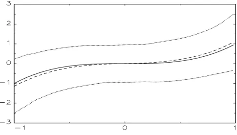
Figure 3: Graphs of fB(x) and Monte Carlo estimates of E ³ ^ fB(x) ´ forh = n¡1=2 (short dashes), h = n¡1=3 (dotted) and h = n¡1=5 (long dashes) with
µ= 100; ¾= 0:1 andn= 500:
Figure 4: Graphs of estimation bands forfB(x)(solid line), the Monte Carlo
estimate ofE³f^B(x)
´
forh=n¡1=3(short dashes) and 95% estimation bands
(dotted) withµ= 100; ¾= 0:1 andn= 500:
![Figure 2: Graphs over the interval [0; 1] of estimation bands for f A (x) (solid line), the Monte Carlo estimate of E ³](https://thumb-us.123doks.com/thumbv2/123dok_us/427884.2549179/25.918.212.725.592.905/figure-graphs-interval-estimation-bands-monte-carlo-estimate.webp)