Constrained estimation via the fused lasso and some generalizations

(1)

Copyright by

Oscar Hernan Madrid Padilla 2017

(2)

The Dissertation Committee for Oscar Hernan Madrid Padilla certifies that this is the approved version of the following dissertation:

Constrained estimation via the fused lasso and some

generalizations

Committee:

James G. Scott , Supervisor Constantine Caramanis

Purnamrita Sarkar Mingyuan Zhou

(3)

Constrained estimation via the fused lasso and some

generalizations

by

Oscar Hernan Madrid Padilla, B.S.

DISSERTATION

Presented to the Faculty of the Graduate School of The University of Texas at Austin

in Partial Fulfillment of the Requirements

for the Degree of

DOCTOR OF PHILOSOPHY

THE UNIVERSITY OF TEXAS AT AUSTIN May 2017

(4)

(5)

Acknowledgments

I would like to thank James Scott, who has been a very supportive advisor. He has been patient, helpful, and has made me feel free about my research. For all this I will always be thankful to him.

I would also like to thank Mingyuan Zhou for his guidance during the early years of my stay in Austin. It was him who encouraged me to start doing research very early on in the PhD program.

I would like to specially acknowledge James Sharpnack fo being such supportive collaborator. I had many stimulating conversations with him that have made me a much better researcher.

I am also very grateful to have worked along side great researchers: Nick Polson, Ryan Tibshirani, and Pradeep Ravikumar. Each with his own style, they have all had great influence in the way I think and do statistical research.

I would like to thank the Statistics and Data Sciences Department (SDS), at The University of Texas at Austin. Its support has made possible every step of my way in the PhD program. In particular, I am very grateful to Michael Daniels and Vicky Keller for making my stay in SDS as smooth as possible.

(6)

grant (DMS-1255187) from the U.S. National Science Foundation. More-over, the motion capture data used in this thesis was obtained from mo-cap.cs.cmu.edu. The database was created with funding from NSF EIA-0196217.

My sincere gratitude also goes to my colleagues, teachers and friends for making my life in Austin very pleasant.

I would like to thank the dissertation committee members for taking the time to read and help me improve this dissertation.

Finally, to my family. My parents Alejandrina Padilla and Jose Madrid. They have provided everything for me. I thank them for their inconditional love and incredible vision of life. To my siblings, thanks for all their encour-agement and love.

(7)

Constrained estimation via the fused lasso and some

generalizations

Publication No.

Oscar Hernan Madrid Padilla, Ph.D. The University of Texas at Austin, 2017

Supervisor: James G. Scott

This dissertation studies structurally constrained statistical estima-tors. Two entwined main themes are developed: computationally efficient algorithms, and strong statistical guarantees of estimators across a wide range of frameworks.

In the first chapter we discuss a unified view of optimization prob-lems that enforces constrains, such as smoothness, in statistical inference. This in turn helps to incorporate spatial and/or temporal information about data.

The second chapter studies the fused lasso, a non-parametric regres-sion estimator commonly used for graph denoising. This has been widely used in applications where the graph structure indicates that neighbor nodes have similar signal values. I prove for the fused lasso on arbitrary graphs,

(8)

an upper bound on the mean squared error that depends on the total vari-ation of the underlying signal on the graph. Moreover, I provide a surro-gate estimator that can be found in linear time and attains the same upper– bound.

In the third chapter I present an approach for penalized tensor de-composition (PTD) that estimates smoothly varying latent factors in multi-way data. This generalizes existing work on sparse tensor decomposition and penalized matrix decomposition, in a manner parallel to the general-ized lasso for regression and smoothing problems. I present an efficient coordinate-wise optimization algorithm for PTD, and characterize its con-vergence properties.

The fourth chapter proposes histogram trend filtering, a novel ap-proach for density estimation. This estimator arises from looking at surro-gate Poisson model for counts of observations in a partition of the support of the data.

The fifth chapter develops a class of estimators for deconvolution in mixture models based on a simple two-step bin-and-smooth procedure, applied to histogram counts. The method is both statistically and compu-tationally efficient. By exploiting recent advances in convex optimization, we are able to provide a full deconvolution path that shows the estimate for the mixing distribution across a range of plausible degrees of smoothness, at far less cost than a full Bayesian analysis.

(9)

Finally, the sixth chapter summarizes my contributions and provides possible directions for future work.

(10)

List of Tables

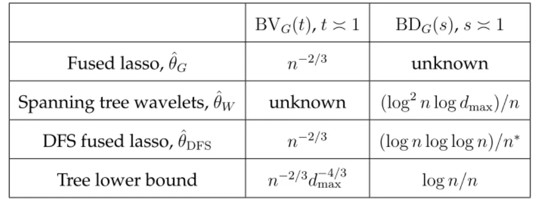
2.1 A summary of the theoretical results derived in this chapter. All rates are on the mean squared error (MSE) scale (Ekθˆ−θ0k2nfor an estimatorθˆ), and for simplicity, are presented under a constant scaling fort, s, the radii in theBVG(t),BDG(s) classes, respectively. The superscript “∗” in the

BDG(s) rate for the DFS fused lasso is used to emphasize that this rate only holds under the assumption thatWn n. Also, we writedmaxto denote the max degree of the graph in question. . . 57 3.1 Comparison of the Frobenius norm error between the true

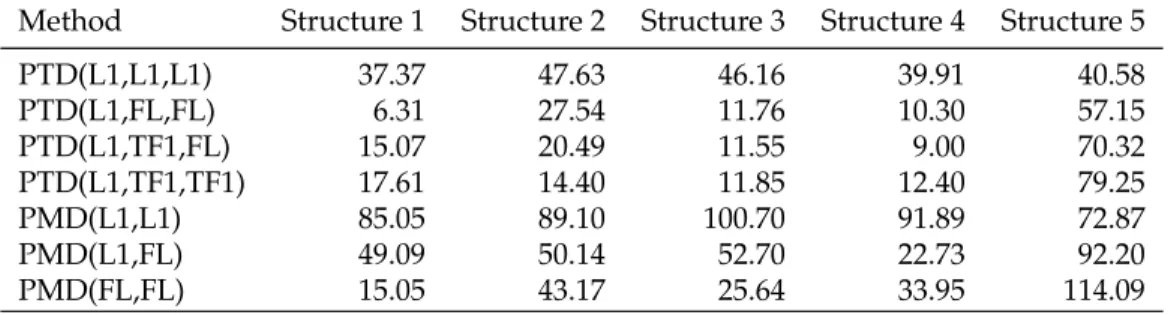
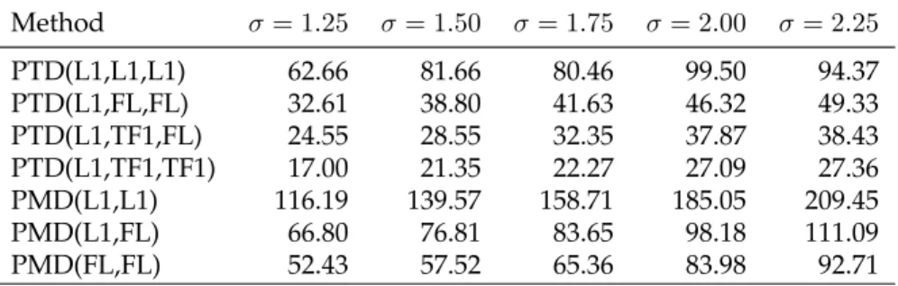
tensor and the estimated tensor using different methods. . . . 87 3.2 Comparison of the Frobenius norm error between the true

tensor and the estimated tensor using for different levels of noise and a fixed structure, averaging over 100 Monte Carlo simulations . . . 88 3.3 Comparison of the Frobenius norm error between the true

tensor and the estimated tensor using different methods, av-eraging over 100 Monte Carlo simulations . . . 89 3.4 Comparison of the Frobenius norm error between the

esti-mated tensor and the test tensor for the moCap datasets . . . . 93 4.1 Mean-squared error×100 on example 1 for histogram trend

filtering withk = 1 and k = 2 versus three other methods: kernel density estimation with bandwidth chosen by cross-validation, kernel density estimation using the normal refer-ence rule, and local polynomial density estimation. . . 116 4.2 Mean-squared error × 100 on example 2 for the same five

methods in Table 4.1. . . 116 4.3 Mean-squared error × 10 on example 1, averaging over 50

MC simulations . . . 117 4.4 Mean-squared error× 100 on example 2, averaging over 50

MC simulations. . . 118 4.5 Mean-squared error × 10 on example 3, averaging over 50

(16)

4.6 Mean-squared error × 10 on example 4, averaging over 50 MC simulations. . . 119 4.7 Time in seconds for Example 1, averaging over 50 MC

simu-lations. . . 119 4.8 Average log-likelihood on test set times10−3_{, averaging over}

50 random training and test sets of sizess%and(100−s)%

respectively. . . 123 5.1 Mean squared error (MSE) between the true and estimated

mixing densities, averaging over 100 Monte Carlo simula-tions, for different methods given samples from density Ex-ample 1. The acronyms here are given the text. The MSE is multiplied by102_{and reported over two intervals containing} 95% and 99% of the mass of the mixing density. . . 150 5.2 Mean squared error (MSE) between the true and estimated

mixing densities, averaging over 100 Monte Carlo simula-tions, for different methods given samples from density Ex-ample 2. The acronyms here are given the text. The MSE is multiplied by103and reported over two intervals containing 95% and 99% of the mass of the mixing density. . . 151 5.3 Mean squared error (MSE) between the true and estimated

mixing densities, averaging over 100 Monte Carlo simula-tions, for different methods given samples from density Ex-ample 3. The acronyms here are given the text. The MSE is multiplied by103_{and reported over two intervals containing} 95% and 99% of the mass of the mixing density. . . 152 5.4 Mean squared error (MSE) between the true and estimated

mixing densities, averaging over 100 Monte Carlo simula-tions, for different methods given samples from density Ex-ample 4. The acronyms here are given the text. The MSE is multiplied by104_{and reported over two intervals containing} 95% and 99% of the mass of the mixing density. . . 153 5.5 Mean squared error, of the normal means estimates, times

100 , averaging over 100 Monte Carlo simulations, for differ-ent methods given samples from example 1. . . 155 5.6 Mean squared error, of the normal means estimates, times

100, averaging over 100 Monte Carlo simulations, for differ-ent methods given samples from example 2. . . 155

(17)

5.7 Mean squared error, of the normal means estimates, times 100, averaging over 100 Monte Carlo simulations, for differ-ent methods given samples from example 3. . . 156 5.8 Mean squared error, of the normal means estimates, times

100, averaging over 100 Monte Carlo simulations, for differ-ent methods given samples from example 4. . . 156

(18)

List of Figures

1.1 Example of image denoising, the left panel corresponds to a noisy input image, the right panel consists of the fused lasso solution. . . 6 1.2 The first two panels show two examples off0 in model (1.5)

plotted on top of the corresponding drawsy, which are dis-played as a normalized histogram. The panels in the second row show from left to right (for a different f0), respectively, the density φ ∗f0 on top of the draws {yi}ni=1, and the den-sityf0 on top of the unobserved draws{µi}ni=1. Hereφis the standard Gaussian density function. . . 9 2.1 The optimized MSE for the DFS fused lasso and Laplacian smoothing

(i.e., MSE achieved by these methods under optimal tuning) is plotted as a function of the total variation of the underlying signal, for each of the three road network graphs. This has been averaged over 50 draws of data

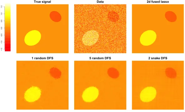
yfor each construction of the underlying signalθ0, and 10 repetitions in constructingθ0 itself. For low values of the underlying total variation, i.e., low SNR levels, the two methods perform about the same, but as the SNR increases, the DFS fused lasso outperforms Laplacian smoothing by a considerable margin. . . 49 2.2 Underlying signal, data, and solutions from the 2d fused lasso and

differ-ent variations on the DFS fused lasso fit over a1000×1000grid. . . 51 2.3 Optimized MSE and runtime for the 2d fused lasso and DFS fused lasso

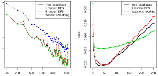
estimators over a 2d grid, as the grid sizen(total number of nodes) varies. 51 2.4 The left panel shows the optimized MSE as a function of the sample size

for the fused lasso over a tree graph, as well as the 1 random DFS and 5 random DFS estimators, and wavelet smoothing. The right panel . . . 55

(19)

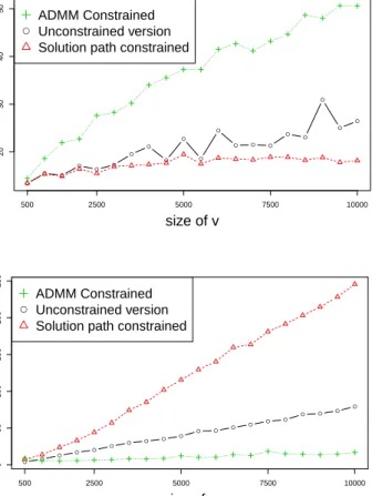
3.1 Panel (a): Frobenius error comparison of the of three differ-ent methods for finding a rank-1 decomposition. These are: Algorithm 1 with the ADMM method from [156], block coor-dinate descent for solving the unconstrained problem (3.11), and Algorithm 1 using the solution path method as described in Section 3.1. Panel (b): For each of the methods, time in sec-onds for solving one problem with a particular choice of tun-ing parameters. Our unconstrained formulation with adap-tive chosen penalties achieves nearly the reconstruction error of the unconstrained formulation with optimal hyperparam-eter choice, but at far less computational cost. . . 79 3.2 Each row gives rise to a different structure by taking the outer

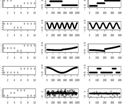
product on the corresponding, horizontally plotted, vectors. . 85 3.3 (a) Time vector for the first factor (b) Loadings matrix for first

factor (c) Time vector for second factor (d) Loadings matrix for second factor. . . 90 4.1 Left panel depicts the estimated density provided by our Bayesian

HTF, withτ selected using DIC, on top of data generated us-ing the density on the third panel. For purposes of compari-son, we also display the Bayesian HTF by itself in the second panel. In this examplen= 4000. . . 110 4.2 Top two panels: the true densities f1 (left) and f2 (right) in

the simulation study, together with samples ofn = 2500from each density. Middle two panels: results of histogram trend filtering for thef1sample (left) and thef2sample (right). Bot-tom two panels: results of kernel density estimation for the f1 sample (left) and thef2 sample (right). In the bottom four panels the reconstruction results are shown on a log scale. . . 115 4.3 Each row of panels above represents an example considered

in this section. For each row the first column shows the true density along withn = 4000draws from the respective den-sity. The second column shows the error for the solution given by HTF(k=1). Similarly, the third column of panels rep-resents the estimate error for W-N. . . 120 4.4 The left panel shows the binned counts for a training set

con-sisting of 75% of the subset of the NYC Taxi data that we used. The right panel shows the counts for the respective test set or remaining 25% of the data. . . 122

(20)

5.1 Example of deconvolution with an`2 _{penalty on the discrete} first derivative (k = 1). The left panel shows the data his-togram together with the fitted marginal density as a solid curve. The right panel shows the histogram of the µi’s to-gether with the estimated mixing measure as a solid curve. . . 138 5.2 Rows A–E show five points along the deconvolution path for

the prostate cancer gene-expression data. The regularization parameter is largest in Row A and gets smaller in each suc-ceeding row. . . 140 5.3 The first three panels show 95%confidence bands and

poste-rior mean from 15000 posteposte-rior samples from a mixture of 10 normals prior on the latent variablesµ. Panels 4-7 then shows the estimated mixing density using the kernel estimator with different bandwidth choices. . . 141 5.4 The first panel shows a histogram of observed data {yi}ni=1

for our first example, and the L1-D marginal density esti-mate plotted on top of the histogram. Here the data has been generated asyi ∼ N(µi,1)where µi is a draw from the mix-ing density. The second panel shows, for this same example, the histogram of{µi}n

i=1 (unobserved draws from the mixing density) and the L1-D estimate of the mixing density plotted on top of it. Panels 3-6 show the respective cases of Examples 2 and 3. The last two panels show the corresponding plots for the L2-D solution and Example 4. . . 147 5.5 For the mixing density illustrated in Example 1 of Figure 5.4

we show the estimated mixing densities of different methods. The top two panels correspond to the estimated mixing den-sities using L2-D and PR algorithms along with latentµ. Bot-tom two panels show the estimated density using MN and FTKD both with the latentµ. For all four panelsn = 105 _{. . . . 148}

(21)

Chapter 1

Introduction

In recent years there has been an increasing interest in the use of pe-nalized methods for different statistical problems. Pepe-nalized methods are characterized by providing models that balance between overfitting and structural constrains on the estimators. This includes, fundamental work in regression analysis, density estimation and dimension reduction. This line of work differs from classical techniques, however, in the use of penalty functions that encourage these estimated solutions to be sparse, structured, or both. As previous work has demonstrated, such regularized estimators usually exhibit a favorable bias-variance tradeoff and can also make the es-timated models themselves much more interpretable to practitioners.

In the one-dimensional case, penalized regression problems have been widely studied in the literature. In most previous work in this area, differ-ent choices of penalties have proven to be successful for specific applica-tions. One of these celebrated penalties is the fused lasso which constrains solutions to be piecewise constants. This can be a very desirable feature for different statistical problems where there is a natural ordering of the ob-servations. For instance, in protein mass spectroscopy and gene expression

(22)

data measured from a microarray, the fused lasso has been used to obtain in-terpretable results. Another widely used penalty is trend filtering that pro-vides piecewise polynomial solutions. Such smooth estimators have found applications in areas as diverse as image processing and demography.

This dissertation studies different statistical problems exploiting some of the penalized likelihood techniques mentioned above, applying these to specific problems particularly related to non-parametric regression, prin-cipal component analysis and density estimation. The goals are twofold. First, we study algorithms, using state of the art techniques from convex optimization, that can provide accurate and fast solutions to the estimation problems mentioned above. Secondly, we aim to study statistical guaran-tees for our algorithms ensuring that with high probability the solutions provided are close, in some metric sense, to the true parameters.

1.1

A regularized likelihood point of view of estimation

The typical framework of statistical inference consists of estimating an unknown parameter θ from a set of observations y. In this work we study different instances of this problem where the parameter lies in a high-dimensional space, which makes estimation difficult, but there is an special structure that can be exploited to perform estimation.

More precisely, we suppose that datay ∈ _Rn_{is given,} _n _∈

(23)

generated as

y ∼ f(θ0), (1.1)

where the true parameter satisfiesθ0 ∈ Θ, and f is a joint density function indexed by parameters in the spaceΘ. Moreover, we assume, in all the set-tings considered here, that the observationsyi,i∈ {1, . . . , n}, are marginally independent.

In many statistical frameworks, in addition to observing the data, practitioners have some prior knowledge about the structure of the true parameter giving rise to the data. We formalize this by saying that there exists a known functionJ : Θ→_Rwhich satisfies

J(θ0) ≤ c,

wherecis an unknown positive constant, which satisfiesc << n. Thus,cis much smaller than the sample size.

In the statistics and machine learning communities, the functionJ is often referred to as penalty, and it is used to incorporate prior beliefs about the problem in hand. For instance, in certain applications one might want to enforce spatial and/or temporal properties of the data.

The first natural question that arises with settings like the ones de-scribed above is: how can the parameter θ0 be estimated? This is usually important for interpretation, visualization, and also prediction tasks related to the data in hand.

(24)

There are two traditional approaches for estimation: Bayesian infer-ence, and regularized likelihood optimization. In this thesis we focus al-most exclusively in the latter.

Consider the interpretation of the penaltyJ as the minus-logarithm of a possibly improper prior. Thus, on the unknown true parameter, we place the prior,

P(θ) ∝ exp(−λ J(θ)), (1.2) for a tuning parameterλ > 0. Combining both (1.1) with (1.2) leads to a Bayesian model which can, in principle, enable estimation via Markov chain Monte Carlo (MCMC) methods. However, such approach might not gener-ally be tractable nor computationgener-ally efficient. Hence, we mainly focus on maximum a posteriori estimators. Thus, estimators arising as

ˆ

θ = argmin_θ_∈_Θ−log_P(y|θ) +λ J(θ). (1.3) The above framework, in a very general way, encompasses the dif-ferent estimation problems that concern the interest of this thesis. Our goal is to provide computational efficient algorithms for solving problems of the form (5.5), together with statistical guarantees that ensure validity of our procedures. The specific focus of our study is on:

• Graph denoisingThis is a normal means estimation problem, where

the data y comes along with a graph structure G. The true parame-terθ0 lies inRn, and the underlying assumption is that signal values

(25)

corresponding to connected nodes in the graphGtend to have similar values. Loosely speaking, the signal θ0 is smooth along the graphG, and we make use of this property for estimation purposes.

• Tensor decompositionIn this setting the data is given in the form of

a three dimensional array,{yi,j,k} ∈ _RL×T×S_{, with}_n ₌_L_×_T _×_{S. Our} goal is to design algorithms to extract low dimensional interpretable features in the presence of noisy measurements.

• Density estimation For the classical problems of deconvolution and

density estimation, I study adaptive non-parametric estimators, em-phasizing the natural assumption that the true model is somehow smooth, but can also have sharp regions.

For all of the above research problems, the key to our work is to en-force smoothness assumptions encoded through appropriate penalties J. The penalties we use enjoy adaptivity to different degrees of smoothness.

1.2

Graph denoising

In many applications, one is given noisy measurements on a net-work, and the goal is to estimate the underlying signal using the network information. The main assumption of graph denoising methods is that the true signal varies smoothly along the graph.

One of the most widely used methods for graph denoising problems, given its attractive computational and statistical properties, is the fused

(26)

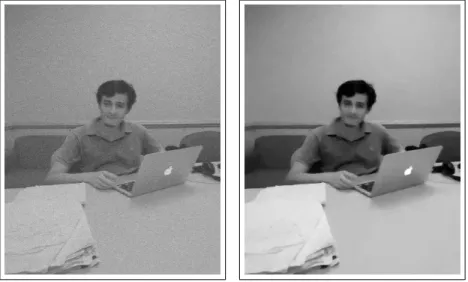
Figure 1.1: Example of image denoising, the left panel corresponds to a noisy input image, the right panel consists of the fused lasso solution.

lasso estimator [137, 118]. This estimator is obtained as the solution of an optimization problem, as (5.5). In such equation, the likelihood part comes from a Gaussian model, while as we will see in Chapter 2, the penalty J encourages neighboring nodes to have similar signal values.

An example of a graph denoising problem is illustrated in Figure 1.1. There we see a noisy input image and the output of using total variation denoising (fused lasso).

While the fused lasso has attracted great attention for the develop-ment of algorithms [28, 74, 8, 136, 90, 87], it is still not known a unifying fast algorithm that can scale well in practice, regardless of the graph. More-over, it has remained as an open question to understand the convergence rates of the fused lasso on general graphs. In this dissertation we fill this

(27)

gap and provide convergence results that hold for any connected graph and any signal. Surprisingly, we will show that such universal guarantees can be attained by a simple procedure that runs in linear time, on the number of edges, for any graph structure.

1.3

Tensor decompositions

Given a data arrayY = {ylts}, practitioners in statistics are often in-terested in extracting low dimensional factors. This is typically done with the purpose of interpretation and prediction. State of the art methods al-low us to do so by using Parafac decompositions. However, an important open question is to provide smooth Parafac decompositions. We address this question by developing convex optimization algorithms that extract smooth low rank decompositions. Such representations can be useful for incorporating spatial and/or temporal information of the data.

The generative model that we study gives rise to a set of observations yl,t,s, as yl,t,s = J X j=1 d∗_ju∗_ljv_tj∗ w∗_sj+el,t,s, , l∈ {1, . . . , L}, t∈ {1, . . . , T}, s∈ {1, . . . , S} (1.4) with unknown hidden vectorsu∗_:j ∈_RL_{, v}∗

:j ∈RT, w

∗

:j ∈RS,j = 1, . . . , J and scalarsd∗_j, j = 1, . . . , J. Motivated for interpretation purposes, we make the additional assumption that latent vectors are discrete evaluations of piece-wise differentiable functions.

(28)

We answer the question of how to estimate these latent factors, by solving a suitable optimization which is a special case of (5.5). The corre-sponding penalty J is a convex non-differentiable function chosen to en-courage sparse and/or smooth factors. However, care needs to be taken as the likelihood is a convex function, which together with the non-differentiability of the penalty posses an estimation challenge.

1.4

Density estimation and deconvolution

Density estimators are one of the most commonly used tools for data exploration. They are widely used as first past tool for visualization, and can also be used for predicting future events.

Formally, we study a non-parametric density estimator of a density f0 that satisfies

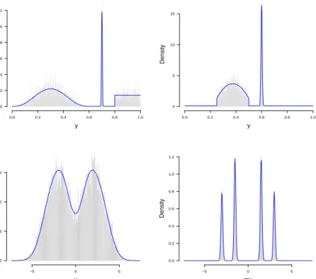
yi, ∼i.i.d f0, i = 1, . . . , n. (1.5) Most practitioners turn to kernel estimators when face with estimatingf0. However, it is well known that kernel estimators cannot properly adapt to different levels of smoothness of the true density. See the first two panels of Figure 1.2 for examples off0 that have different levels of smoothness in their domain.

One of the reasons why kernel estimators are widely used in prac-tice is because adaptive estimators are computationally intense. This leads to the natural question: can we provide a computationally efficient

(29)

adap-Figure 1.2: The first two panels show two examples of f0 in model (1.5) plotted on top of the corresponding drawsy, which are displayed as a nor-malized histogram. The panels in the second row show from left to right (for a differentf0), respectively, the densityφ ∗f0 on top of the draws {yi}ni=1, and the densityf0 on top of the unobserved draws{µi}ni=1. Here φ is the standard Gaussian density function.

y Density 0.0 0.2 0.4 0.6 0.8 1.0 0 2 4 6 8 10 12 y Density 0.0 0.2 0.4 0.6 0.8 1.0 0 5 10 15 y Density −5 0 5 0.00 0.05 0.10 0.15 mu Density −5 0 5 0.0 0.2 0.4 0.6 0.8 1.0 1.2

tive density estimator? We propose a possible answer to this question in Chapter 4.

A further difficulty to density estimation in practice occurs when an additional noise level is added to model (1.5). Thus, the datayis actually a

(30)

noisy version of unobserved measurements{µi}fromf0. Specifically, yi | µi ∼i.i.d φ(yi|µi),

µi ∼i.i.d f0. (1.6) where φ is known distribution. In this modified context, estimating f0 is known as deconvolution. And although (1.6) seems like a slightly more complicated model than (1.5), it is well known that deconvolution is a much more difficult problem. The author in [56] showed that the convergence rates in deconvolution problems, in`2loss function, are in the order of pow-ers of (logn)−1 as opposed to powers of n−1, as it is the case for density estimation.

While the theoretical results, in the way of convergence rates, are very discouraging, deconvolution has been an extensively studied statisti-cal problem [78, 58, 56, 107, 63, 39, 52]. One important question is: how can we construct computationally feasible adaptive deconvolution estimators? This is the focus of Chapter 5, where we propose a novel estimator that also enjoys some desirable statistical properties.

Another important aspect of deconvolution is its connection with the normal means estimation problem, a setting of interest in biological appli-cations (e.g. [48, 123]). This consists in estimating {µi}in the case in which φis the standard Gaussian kernel.

The role of deconvolution in the normal means estimation problem is understood through Tweedie’s formula which states that

E(µi |yi) =yi+

d

dylogm(yi) = yi+

m0(yi)

(31)

where m(·) := φ∗f0 =

R

φ(· | µ)f0(µ)d µis the marginal density of the data. Thus, having an estimate of the mixing density (f0) immediately gives estimates of{µi}by a straightforward application of Equation (1.7).

In this work we will provide a deconvolution estimator with strong empirical evidence that can be competitive for the normal means estimation problem. It is beyond the scope of our work to mathematically characterize such performance, but rather to offer a reasonable well behave estimator.

We conclude this section with an example that illustrates the diffi-culty of deconvolution. This is shown in the bottom two panels of Figure 1.5. The left panel shows the observed data{yi}as a histogram along with the true marginal density. The right panel shows the latent variables{µi} as a histogram with the true mixing density. It is clear from these plots that the observed data significantly obscures the actually mixing density, exem-plifying how challenging deconvolution can be.

1.5

Total variation penalties

As explained before, the focus of this thesis is to develop efficient al-gorithms, with statistical guarantees, that overcome some of the challenges and limitations of state of the art methods in the frameworks of graph de-noising, low rank tensor decompositions, and deconvolution and density estimation. We do so by proposing estimators that come as the solutions to optimization problems of the form (5.5) using penalties that enforce smooth

(32)

solutions. The penalty functions that we use are extensions, or generaliza-tions, of the fused lasso penalty introduced by [118, 102, 137]. This relies on the idea of total variation, which we briefly depict next.

Given a functionf : [0,1]→_R, we define its total variation as

TV(f) := sup (_N₋₁ X i=1 |f(xi)−f(xi+1)| : x1 = 0< x2 < . . . < xN = 1, N ∈N ) (1.8) and iff is differentiable, then it can be proven that

TV(f) =

Z 1

0

|f0(t)|dt.

It is clear from its definition that “smoother” functions will tend to have smaller total variation, hence that the total variation offers a natural alter-native as regularization in statistical estimation. In such context, it was first introduced by [101] for one-dimensional non-parametric regression. How-ever, one of the possible limitations of using such penalties is that it re-quires to have an interval, or topological space for the signal’s domains, over which partitions are considered and a supremum is taken. This con-strains the range of applicability of the TV penalty. This will be more ev-ident in Chapter 2, where we deal with general graph structures. Fortu-nately, [137] proposed a penalty function, which we refer to as the fussed lasso, that is defined as

FL(θ) :=

N−1

X

i=1

(33)

Hence, instead of working with a complicated definition as (1.8), the ex-pression in (1.9) offers a discrete penalty that can easily be generalized to more general contexts, which has led to more computationally efficient al-gorithms, see [79, 74, 140, 149].

1.6

Outline

The rest of this thesis is organized as follows.

Chapter 2 starts by presenting a brief introduction, followed by a statement of the general graph denoising problem. The chapter then sum-marizes our contributions before moving to discuss modeling assumptions, notation, and previous work. The latter includes an overview of the liter-ature on the fused lasso focusing in computational and theoretical aspects. All of this constitutes Section 2.1. From there, in Section 2.2, we prove a sim-ple but key lemma relating the`1norm (and`0) norm of differences on a tree and a chain induced by running the depth-first search algorithm (DFS). We then define the DFS fused lasso estimator. In Section 2.3, we derive mean squared error (MSE) rates for the DFS fused lasso, and the fused lasso over the original graphGin question, for signals of bounded variation. We also derive lower bounds for the minimax MSE rate over trees. Section 2.4 pro-ceeds similarly, but for signals with bounded differences. In Section 2.5, we cover numerical experiments, and in Section 2.6, we summarize our work and also describe some potential extensions.

(34)

Chapter 3 begins with a discussion of tensor decompositions in Sec-tion 3.1, and an overview of previous work in SecSec-tion 3.2. We then introduce the basic notation on tensors in Section 3.3, which leads to our formulation of rank-1 penalized tensor decomposition (PTD) in Section 3.4. From there, Section 3.5 presents two formulations of our PTD: one with penalties as con-strained set, and one with the penalties in the objective function. Section 3.6 provides a convergence analysis for the case of rank-1 decompositions. In Section 3.7 we perform an extensive simulation study highlighting the strengths and weaknesses of our approach. Section 3.8 validates our me-thods on two real data examples. The first consists of flu hospitalizations in Texas. The second example is based on motion capture data. Finally, Section 3.9 provides a brief discussion of what was presented in the chapter.

In Chapter 4 we study a novel approach for density estimation. Sec-tion 4.1 summarizes our contribuSec-tions. In one dimension, our approach is introduced in Section 4.2. The chapter then discusses, relevant, previ-ous work on non-parametric density estimation. This is the main focus of Section 4.3. It includes aspects such as adaptive and penalized likelihood estimators, log-density estimation, and Lindsey’s method. Section 4.4 pro-vides our main theoretical result of the chapter. In Section 4.5, we discuss model selection aspects of our proposed method. Extensions of our one di-mensional approach are discussed in Sections 4.6 and 4.7, where we present a Bayesian view and a 2-dimensional estimator respectively. In Section 4.8 we perform one-dimensional validations of our method versus kernel and

(35)

adaptive methods in the literature. This section also includes a real data ex-ample on NYC taxi data. The conclusion of the chapter is given in Section 4.9.

Chapter 5 studies deconvolution problems. Section 5.1 presents the statistical model of interest, and the relevant literature is discussed in Sec-tion 5.2. Our approach is developed with great details in SecSec-tion 5.3. A sensitivity analysis with real data is performed in Section 5.4. Our consis-tency result is the main theme of Section 5.6. We then provide simulation experiments in Section 5.6. These consist of examples estimating the mix-ing density, and also for the normal means estimation problem. We then conclude the chapter with a discussion in Section 5.7.

Finally, our contributions are summarized in Chapter 6, where we also present some open question that are left for future work.

(36)

Chapter 2

The DFS Fused Lasso: Linear-Time Denoising

over General Graphs

This chapter, based on the working paper [100], studies graph de-noising estimators in general graphs. Specifically, the fused lasso, also known as (anisotropic) total variation denoising, which is widely used for piece-wise constant signal estimation with respect to a given undirected graph. The fused lasso estimate is highly nontrivial to compute when the under-lying graph is large and has an arbitrary structure. But for a special graph structure, namely, the chain graph, the fused lasso—or simply, 1d fused lasso—can be computed in linear time. In this chapter, we establish a sur-prising connection between the total variation of a generic signal defined over an arbitrary graph, and the total variation of this signal over a chain graph induced by running depth-first search (DFS) over the nodes of the graph. Specifically, we prove that for any signal, its total variation over the induced chain graph is no more than twice its total variation over the original graph. This connection leads to several interesting theoretical and computational conclusions. Denoting bymandnthe number of edges and nodes, respectively, of the graph in question, our result implies that for an underlying signal with total variation t over the graph, the fused lasso

(37)

achieves a mean squared error rate of t2/3_n−2/3_{. Moreover, precisely the} same mean squared error rate is achieved by running the 1d fused lasso on the induced chain graph from running DFS. Importantly, the latter estima-tor is simple and computationally cheap, requiring onlyO(m) operations for constructing the DFS-induced chain and O(n) operations for comput-ing the 1d fused lasso solution over this chain. Further, for trees that have bounded max degree, the error rate oft2/3n−2/3 cannot be improved, in the sense that it is the minimax rate for signals that have total variationt over the tree. Finally, we establish several related results—for example, a similar result for a roughness measure defined by the`0 norm of differences across edges in place of the the total variation metric.

2.1

Statistical model

We study the graph denoising problem, i.e., estimation of a signal θ0 ∈Rnfrom noisy data

yi =θ0,i+i, i= 1, . . . , n, (2.1) when the components ofθ0are associated with the vertices of an undirected, connected graphG= (V, E).

Throughout, a graphG= (V, E)consists of two sets: a set of nodesV, and a set of edgesE. Without loss of generality we assumeV ={1, . . . , n}. Moreover, E consists of unordered pairs (undirected), called edges, (i, j)

(38)

a sequencei1, . . . , iK, for someK, such that(il, il+1)∈Eforl = 1, . . . , K−1. The graphGis called connected if there is a path between any two pair of nodes.

Versions of (2.1) arise in diverse areas of science and engineering, such as gene expression analysis, protein mass spectrometry, and image de-noising. The problem is also archetypal of numerous internet-scale machine learning tasks that involve propagating labels or information across edges in a network (e.g., a network of users, web pages, or YouTube videos).

Methods for graph denoising have been studied extensively in ma-chine learning and signal processing. In mama-chine learning, graph kernels have been proposed for classification and regression, in both supervised and semi-supervised data settings (e.g., [10, 130, 155, 154]). In signal pro-cessing, a considerable focus has been placed on the construction of wavelets over graphs (e.g., [30, 27, 60, 67, 125, 126]). We will focus our study on the

fused lassoover graphs, also known as (anisotropic)total variationdenoising

over graphs. Proposed by [118] in the signal processing literature, and [139] in the statistics literature, the fused lasso estimate is defined by the solution of a convex optimization problem,

ˆ θG = argmin θ∈_Rn 1 2ky−θk 2 2+λk∇Gθk1, (2.2) where y = (y1, . . . , yn) ∈ Rn the vector of observed data, λ ≥ 0 is a tun-ing parameter, and ∇G ∈ Rm×n is the edge incidence matrix of the graph G. Note that the subscript on the incidence matrix∇G and the fused lasso

(39)

solutionθˆGin (2.2) emphasize that these quantities are defined with respect to the graphG. The edge incidence matrix∇Gcan be defined as follows, us-ing some notation and terminology from algebraic graph theory (e.g., [64]). First, we assign an arbitrary orientation to edges in the graph, i.e., for each edge e ∈ E, we arbitrarily select one of the two joined vertices to be the head, denotede+, and the other to be the tail, denotede−. Then, we define a row(∇G)eof∇G, corresponding to the edgee, by

(∇G)e,e+ = 1, (∇_G)_e,e− =−1, (∇_G)_e,v = 0 for allv 6=e+, e−,

for eache∈E. Hence, for an arbitraryθ∈_Rn_{, we have}

k∇Gθk1 =

X

e∈E

|θe+ −θ_e−|.

We can see that the particular choice of orientation does not affect the value

k∇Gθk1, which we refer to as thetotal variationofθover the graphG.

2.1.1 Summary of results

We will wait until Section 2.1.3 to give a detailed review of litera-ture, both computational and theoretical, on the fused lasso. Here we sim-ply highlight a key computational aspect of the fused lasso to motivate the main results in this chapter. The fused lasso solution in (2.2), for a graph Gof arbitrary structure, is highly nontrivial to compute. For a chain graph, however, the fused lasso solution can be computed in linear time (e.g., using dynamic programming or specialized taut-string methods).

(40)

The question we answer is: how can we use this fact to our advan-tage, when seeking to solve (2.2) over an arbitrary graph? Given a generic graph structureGthat has medges and n nodes, it is obvious that we can define a chain graph by running depth-first search (DFS) over the nodes. Far less obvious is that, for any signal, its total variation over the DFS-induced chain graph never exceeds twice its total variation over the original graph. This fact, which we prove, has the following three notable consequences (the first being computational, and next two statistical).

1. No matter the structure ofG, we can denoise any signal defined over this graph inO(m+n)operations:O(m)operations for DFS andO(n)

operations for the 1d fused lasso on the induced chain. We call the corresponding estimator—the 1d fused lasso run on the DFS-induced chain—theDFS fused lasso.

2. For an underlying signal θ0 that generates the data, as in (2.1), such thatθ0 ∈BVG(t), whereBVG(t)is the class of signals with total varia-tion at mostt, defined in (2.4), the DFS fused lasso estimator has mean squared error (MSE) on the order oft2/3n−2/3.

3. For an underlying signalθ0 ∈BVG(t), the fused lasso estimator over the original graph, in (2.2), also has MSE on the order oft2/3_n−2/3_.

The fact that such a fast rate, t2/3_n−2/3_{, applies for the fused lasso} estimator over any connected graph structure is somewhat surprising. It

(41)

implies that the chain graph represents the hardest graph structure for de-noising signals of bounded variation—at least, hardest for the fused lasso, since as we have shown, error rates on general connected graphs can be no worse than the chain rate oft2/3_n−2/3_.

We also complement these MSE upper bounds with the following minimax lower bound over trees.

4. WhenGis a tree of bounded max degree, the minimax MSE over the classBVG(t)scales at the ratet2/3n−2/3. Hence, in this setting, the DFS fused lasso estimator attains the optimal rate, as does the fused lasso estimator overG.

Lastly, we prove the following for signals with a bounded number of nonzero edge differences.

5. For an underlying signalθ0 ∈BDG(s), whereBDG(s)is the class of sig-nals with at mostsnonzero edge differences, defined in (2.5), the DFS fused lasso (under a condition on the spacing of nonzero differences over the DFS-induced chain) has MSE on the order of

s(logs+ log logn) logn/n+s3/2/n.

When G is a tree, the minimax MSE over the class BDG(s) scales as slog(n/s)/n. Thus, in this setting, the DFS fused lasso estimator is only off by alog lognfactor provided thatsis small.

(42)

This DFS fused lasso gives us anO(n)time algorithm for nearly min-imax rate-optimal denoising over trees. On paper, this only saves a factor of O(logn)operations, as recent work (to be described in Section 2.1.3) has pro-duced anO(nlogn)time algorithm for the fused lasso over trees, by extend-ing earlier dynamic programmextend-ing ideas over chains. However, dynamic programming on a tree is (a) much more complex than dynamic program-ming on a chain (since it relies on sophisticated data structures), and (b) no-ticeably slower in practice than dynamic programming over a chain, espe-cially for large problem sizes. Hence there is still a meaningful difference— both in terms of simplicity and practical computational efficiency—between the DFS fused lasso estimator and the fused lasso over a generic tree.

For a general graph structure, we cannot claim that the statistical rates attained by the DFS fused lasso estimator are optimal, nor can we claim that they match those of fused lasso over the original graph. As an example, recent work (to be discussed in Section 2.1.3) studying the fused lasso over grid graphs shows that estimation error rates for this problem can be much faster than those attained by the DFS fused lasso (and thus the minimax rates over trees). What should be emphasized, however, is that the DFS fused lasso can still be a practically useful method for any graph, running in linear time (in the number of edges) no matter the graph structure, a scaling that is beneficial for truly large problem sizes.

(43)

2.1.2 Assumptions and notation

Our theory will be primarily phrased in terms of the mean squared error (MSE) an estimatorθˆof the mean parameterθ0 in (2.1), assuming that = (1, . . . , n)has i.i.d. mean zero sub-Gaussian components, i.e.,

E(i) = 0, and P(|i|> t)≤Mexp −t2/(2σ2), all t≥0, (2.3)

fori= 1, . . . , n, and constantsM, σ >0. The MSE ofθˆwill be denoted, with a slight abuse of notation, by

kθˆ−θ0k2n =

1

nk

ˆ

θ−θ0k22. (In general, for x ∈ _Rn_{, we denote its scaled} _`

2 norm bykxkn=kxk2/

√

n.) Of course, the MSE will depend not only on the estimatorθˆin question but also on the assumptions that we make aboutθ0. We will focus our study on two classes of signals. The first is the bounded variation class, defined with respect to the graphG, and a radius parametert >0, as

BVG(t) ={θ ∈Rn :k∇Gθk1 ≤t}. (2.4) The second is thebounded differences class, defined again with respect to the graphG, and a now a sparsity parameters >0, as

BDG(s) ={θ ∈Rn :k∇Gθk0 ≤s}. (2.5) We call measure of roughness used in the bounded differences class the

(44)

metric by the`0norm, i.e.,

k∇Gθk0 =

X

e∈E

1{θe+ 6=θ_e−},

which counts the number of nonzero edge differences that appear in θ. Hence, we may think of the former class in (2.4) as representing a type of weak sparsity across these edge differences, and the latter class in (2.5) as representing a type of strong sparsity in edge differences.

When dealing with the chain graph, onn vertices, we will use the following modifications to our notation. We write ∇1d ∈R(n−1)×n for the

edge incidence matrix of the chain, i.e.,

∇1d =      −1 1 0 . . . 0 0 −1 1 . . . 0 .. . . .. ... 0 0 . . . −1 1      . (2.6)

We also writeθˆ1dfor the solution of the fused lasso problem in (2.2) over the chain, also called the1d fused lassosolution, i.e., to be explicit,

ˆ θ1d = argmin θ∈_Rn 1 2ky−θk 2 2+λ n−1 X i=1 |θi+1−θi|. (2.7) We writeBV1d(t)andBD1d(s)for the bounded variation and bounded dif-ferences classes with respect to the chain, i.e., to be explicit,

BV1d(t) ={θ ∈Rn :k∇1dθk1 ≤t},

BD1d(s) ={θ ∈Rn :k∇1dθk0 ≤s}.

Lastly, in addition to the standard notationan =O(bn), for sequences an, bnsuch thatan/bnis upper bounded fornlarge enough, we usean bnto

(45)

denote that bothan =O(bn)anda−n1 =O(b

−1

n ). Also, for random sequences An, Bn, we useAn=OP(Bn)to denote thatAn/Bnis bounded in probability.

2.1.3 Related work

Since its inception in the signal processing and statistics communities in [118] and [139], respectively, there has been an impressive amount of work on total variation penalization and the fused lasso. We do not attempt to give a complete coverage, but point out some relevant computational and theoretical advances, covering the two categories separately.

Computational. On the computational side, it is first worth pointing out

that there are multiple efficient algorithms for solving the fused lasso prob-lem over a chain graph, i.e., the 1d fused lasso probprob-lem. The authors in [33] derived an algorithm based on a “taut string” perspective that solves the 1d fused lasso problem inO(n)time (but, the fact that their taut string method solves the 1d fused lasso problem was not explicitly stated in the work). This was later extended by [28, 8] to allow for arbitrary weights in both of the individual penalty and loss terms. The work in [74] proposed an entirely differentO(n)time algorithm for the fused lasso based on dynamic programming. The taut string and dynamic programming algorithms are extremely fast in practice (e.g., they can solve a 1d fused lasso problem with nin the tens of millions in just a few seconds on a standard laptop).

(46)

[74] to solve the fused lasso problem on a tree. This algorithm is theoret-ically very efficient, withO(nlogn) running time, but the implementation that achieves this running time (we have found) can be practically slow for large problem sizes, compared to dynamic programming on a chain graph. Alternative implementations are possible, and may well improve practical efficiency, but as far as we see it, they will all involve somewhat sophisti-cated data structures in the “merge” steps in the forward pass of dynamic programming.

The authors in [8] extended (though not in the same direct manner) fast 1d fused lasso optimizers to work over grid graphs, using operator splitting techniques like Douglas-Rachford splitting. Their techniques ap-pear to be quite efficient in practice, and the authors provide thorough com-parisons and a thorough literature review of related methods. Over general graphs structures, many algorithms have been proposed, e.g., to highlight a few: [23] described a direct algorithm based on a reduction to paramet-ric max flow programming; [70, 141] gave solution path algorithms (tracing out the solution in (2.2) over allλ∈[0,∞]); [24] described what can be seen as a kind of preconditioned ADMM-style algorithm; [88] described an ac-tive set approach; [136] leveraged fast 1d fused lasso solvers in an ADMM decomposition over trails of the graph; most recently, [90] derived a new method based on graph cuts. We emphasize that, even with the advent of these numerous clever computational techniques for the fused lasso over general graphs, it is still far slower to solve the fused lasso over an arbitrary

(47)

graph than it is to solve the fused lasso over a chain.

Theoretical. On the theoretical side, it seems that the majority of

statis-tical theory on the fused lasso can be placed into two categories: analysis of changepoint recovery, and analysis of MSE. Some examples of works fo-cusing on changepoint recovery are [113, 68, 109, 116]. The statistical theory will concern MSE rates, and hence we give a more detailed review of related literature for this topic.

We begin with results for chain graphs. [102] proved, whenθ0 ∈BV1d(t), that the 1d fused lasso estimator estimatorθ1dˆ withλt−1/3n1/3satisfies

kθˆ1d−θ0k2n=OP(t

2/3_n−2/3₎_.

(2.8) This is indeed the minimax MSE rate for the class BV1d(t), as implied by the minimax results in [45]. (For descriptions of the above upper bound and this minimax rate in a language more in line with that of the current paper, see [141].) Recently, [93] improved on earlier results for the bounded differences class in [32], and proved that whenθ0 ∈BD1d(s), the 1d fused lasso estimatorθ1dˆ withλ(nWn)1/4 satisfies

kθˆ1d−θ0k2n=OP

s n

(logs+ log logn) logn+pn/Wn

, (2.9) whereWndenotes the minimum distance between positions at which nonzero differences occur inθ0, more precisely,

(48)

When these nonzero differences or “jumps” inθ0 are evenly spaced apart, we haveWnn/s, and the above becomes, forλ

√

ns−1/4_,

kθˆ1d−θ0k2n =OP

s(logs+ log logn) logn

n +

s3/2 n

. (2.10) This is quite close to the minimax lower bound, whose rate isslog(n/s)/n, that we establish for the class BD1d(s), in Theorem 2.4.3. (The minimax lower bound that we prove this theorem actually holds beyond the chain graph, and applies to tree graphs). We can see that the 1d fused lasso rate in (2.10) is only off by a factor oflog logn, provided thatsdoes not grow too fast (specifically,s=O((lognlog logn)2)).

Beyond chain graphs, the story is in general much less clear, how-ever, interesting results are known in special cases. For a d-dimensional grid graph, withd≥ 2, [71] recently improved on results of [149], showing that forθ0 ∈BVG(t)∩BDG(s), the fused lasso estimatorθˆGoverGsatisfies

kθˆG−θ0k2n =OP min{t, s}log a n n . (2.11)

whenλloga/2n, wherea= 2ifd= 2, anda= 1ifd≥3. A minimax lower bound on the MSE rate for theBVG(t)class over a gridGof dimensiond≥2 was established to betplog(n/t)/n, by [119]. This makes the rate achieved by the fused lasso in (2.11) nearly optimal for bounded variation signals, off by at most alog3/2nfactor whend= 2, and alognfactor whend≥3.

Other work in [149, 71] also derived MSE rates for the fused lasso over several other graph structures, such as Erdos-Renyi random graphs,

(49)

Ramanujan d-regular graphs, star graphs, and complete graphs. As it is perhaps the most relevant to our goals in this chapter, we highlight the MSE bound from [149] that applies to arbitrary connected graphs. Their Theorem 3 implies, for a generic connected graphG,θ0 ∈BVG(t), that the fused lasso estimatorθˆGoverGwithλ

√ nlognsatisfies kθGˆ −θ0k2_n=O_P t r logn n . (2.12)

(See Appendix A.1 for details.) In Theorem 2.3.2, we show that the uni-versaltn−1/2 rate (ignoring log terms) in (2.12) for the fused lasso over an arbitrary connected graph can be improved tot2/3n−2/3. In Theorem 2.3.1, we show that the same rate can indeed be achieved by a simple, linear-time algorithm: the DFS fused lasso.

2.2

The DFS fused lasso

In this section, we define the DFS-induced chain graph and the DFS fused lasso.

2.2.1 Tree and chain embeddings

We start by studying some of the fundamental properties associated with total variation on general graphs, and embedded trees and chains. Given a graph G = (V, E), let T = (V, ET) be an arbitrary spanning tree ofG. It is clear that for any signal, its total variation of overT is no larger

(50)

than its total variation overG, k∇Tθk1 = X e∈ET |θe+ −θ_e−| ≤ X e∈E |θe+−θ_e−|=k∇_Gθk₁, for all θ ∈_Rn. (2.13) The above inequality, albeit very simple, reveals to us the following impor-tant fact: if the underlying meanθ0in (2.1) is assumed to be smooth with re-spect to the graphG, inasmuch ask∇Gθ0k1 ≤t, then it must also be smooth with respect to any spanning treeT ofG, sincek∇Tθ0k1 ≤t. Roughly speak-ing, computing the fused lasso solution in (2.2) over a spanning treeT, in-stead ofG, would therefore still be reasonable for the denoising purposes, as the meanθ0would still be smooth overT according to the total variation metric.

The same property as in (2.14) also holds if we replace total variation by the cut metric:

k∇Tθk0 = X e∈ET 1{θe+ 6=θ_e−} ≤ X e∈E 1{θe+ 6=θ_e−}=k∇_Gθk₀, for all θ ∈_Rn. (2.14) Thus for the meanθ0, the property k∇Gθ0k0 ≤sagain impliesk∇Tθ0k0 ≤s for any spanning treeT ofG, and this would again justify solving the fused lasso overT, in place ofG, assuming smoothness ofθ0 with respect to the cut metric in the first place.

Here we go one step further than (2.13), (2.14), and assert that anal-ogous properties actually hold for specially embedded chain graphs. The next lemma gives the key result.

(51)

Lemma 2.2.1. LetG = (V, E)be a connected graph, where recall we write V =

{1, . . . , n}. Consider depth-first search (DFS) run onG, and denote by v1, . . . , vn

the nodes in the order in which they are reached by DFS. Hence, DFS first visitsv1,

thenv2, then v3, etc. This induces a bijectionτ : {1, . . . , n} → {1, . . . , n}, such

that

τ(i) = vi, for all i= 1, . . . , n.

LetP ∈_Rn×n_{denote the permutation associated with}_τ_{. Then it holds that}

k∇1dP θk1 ≤2k∇Gθk1, for all θ ∈Rn, (2.15)

as well as

k∇1dP θk0 ≤2k∇Gθk0, for all θ ∈Rn. (2.16)

Proof. The proof is simple. Observe that

k∇1dP θk1 =

X

i=1,...,n−1

|θτ(i+1)−θτ(i)|, (2.17) and consider an arbitrary summand|θτ(i+1)−θτ(i)|. There are now two cases to examine. First, supposeτ(i)is not a leaf node, andτ(i+1)has not yet been visited by DFS; then there is an edgee∈Esuch that{e−, e+}={τ(i), τ(i+ 1)}, and |θτ(i+1)−θτ(i)|=|θe+ −θ_e−|. Second, suppose that either τ(i) is a leaf

node, or all of its neighbors have already been visited by DFS; then there is a path p = {p1, . . . , pr}in the graph such that p1 = τ(i), pr = τ(i+ 1), and each{pj, pj+1} ∈E,j = 1, . . . , r−1, so that by the triangle inequality

|θτ(i+1)−θτ(i)| ≤ r−1

X

j=1

(52)

Applying this logic over all terms in the sum in (2.17), and invoking the fundamental property that DFS visits each edge a most twice (e.g., Chapter 22 of [29]), we have established (2.15). The proof for (2.16) follows from precisely the same arguments.

Example 1. The proof behind Lemma 2.2.1 can also be clearly demonstrated

through an example. We considerGto be a binary tree graph with n = 7

nodes, shown below, where we have labeled the nodes according to the order in which they are visited by DFS (i.e., so that hereP is the identity).

1 2 3 4 5 6 7 In this case, k∆1dθk1 = 6 X i=1 |θi+1−θi| ≤ |θ2 −θ1|+|θ3−θ2|+ |θ3−θ2|+|θ4−θ2| + |θ4−θ2|+|θ2−θ1|+|θ5−θ1| +|θ6−θ5|+ |θ6 −θ5|+|θ7 −θ5| ≤2X e∈G |θe+ −θ_e−|= 2k∇_Gθk₁,

where in the inequality above, we have used triangle inequality for each term in parentheses individually.

(53)

2.2.2 The DFS fused lasso

We define the DFS fused lasso estimator,θˆDFS, to be the fused lasso estimator over the chain graph induced by running DFS on G. Formally, ifτ denotes the bijection associated with the DFS ordering (as described in Lemma 2.2.1), then the DFS-induced chain graph can be expressed asC = (V, EC)whereV ={1, . . . , n}andEC ={{τ(1), τ(2)}, . . . ,{τ(n−1), τ(n)}}. Denoting byP the permutation matrix associated withτ, the edge incidence matrix ofCis simply∇C =∇1dP, and the DFS fused lasso estimator is given by ˆ θDFS = argmin θ∈_Rn 1 2ky−θk 2 2+λk∇1dP θk1 = P> argmin θ∈Rn 1 2kP y−θk 2 2+λ n−1 X i=1 |θi+1−θi| ! . (2.18)

Therefore, we only need to compute the 1d fused lasso estimator on a per-muted data vectorP y, and apply the inverse permutation operatorP>, in order to computeθDFS.ˆ

Given the permutation matrixP, the computational cost of (2.18) is O(n), since, to recall the discussion in Section 2.1.3, the 1d fused lasso prob-lem (2.7) can be solved inO(n)operations with dynamic programming or taut string algorithms. The permutation P is obtained by running DFS, which requires O(m)operations, and makes the total computation cost of the DFS fused lasso estimatorO(m+n).

(54)

same graphG, we must only run DFS once, and all subsequent estimates on the induced chain require justO(n)operations.

The bounds in (2.15), (2.16) for the DFS chain are like those in (2.13), (2.14) for spanning trees, and carry the same motivation as that discussed above for spanning trees, beneath (2.13), (2.14): if the meanθ0is assumed to be smooth with respect tot, insofar as its total variation satisfiesk∇Gθ0k1 ≤t, then denoising with respect toCwould also be reasonable, in that

k∇1dP θ0k1 ≤2t; the same can be said for the cut metric. However, it is the rapidO(m+n)computational cost of the DFS fused lasso, and also the sim-plicity of the dynamic programming and taut string algorithms for the 1d fused lasso problem (2.7), that makes (2.15), (2.16) particularly appealing compared to (2.13), (2.14). To recall the discussion in Section 2.1.3, the fused lasso can in principle be computed efficiently over a tree, inO(nlogn) op-erations using dynamic programming, but this requires a much more cum-bersome implementation and in practice we have found it to be noticeably slower.

2.2.3 Running DFS on a spanning tree

We can think of the induced chain graph, as described in the last section, as being computed in two steps:

(i) run DFS to compute a spanning treeT ofG;

(55)

Clearly, this is the same as running DFS onG to define the induced chain C, so decomposing this process into two steps as we have done above may seem odd. But this decomposition provides a useful perspective because it leads to the idea that we could compute the spanning treeT in Step (i) in any fashion, and then proceed with DFS on T in Step 2 in order to define the chainC. Indeed, any spanning tree in Step (i) will lead to a chainCthat has the properties (2.15), (2.16) as guaranteed by Lemma 2.2.1. This may be of interest if we could compute a spanning treeT that better represents the topology of the original graph G, so that the differences over the eventual chainCbetter mimicks those overG.

An example of a spanning tree whose topology is designed to re-flect that of the original graph is a low-stretch spanning tree. Current in-terest on low-stretch spanning trees began with the breakthrough results in [54]; most recently, [2] showed that a spanning tree with average stretch

O(lognlog logn)can be computed inO(mlognlog logn)operations. In

Sec-tion 5.6.1, we investigate low-stretch spanning trees experimentally.

In Section 2.6.4, we discuss a setting in which the fused lasso problem (2.2) has arbitrary penalty weights, which gives rise to a weighted graphG. In this setting, an example of a spanning tree that can be crafted so that its edges represent important differences in the original graph is a maximum spanning tree. Prim’s and Kruskal’s minimum spanning tree algorithms, each of which takeO(mlogn)time [29], can be used to compute a maximum spanning tree after we negate all edge weights.

(56)

2.2.4 Averaging multiple DFS estimators

Notice that several DFS-induced chains can be formed from a single seed graphG, by running DFS itself on Gwith different random starts (or random decisions about which edge to follow at each step in DFS), or by computing different spanning treesT of G (possibly themselves random-ized) on which we run DFS, or by some combination, etc. Denoting by

ˆ

θ(1)_DFS,θˆ(2)_DFS, . . . ,θˆ(K)_DFSthe DFS fused lasso estimators fit toK different induced chains, we might believe that the average estimator,(1/K)PK

k=1θˆ (k) DFS, will have good denoising performance, as it incorporates fusion at each node in multiple directions. In Section 5.6.1, we demonstrate that this intuition holds true (at least, across the set of experiments we consider).

2.3

Analysis for signals of bounded variation

Throughout this section, we assume that the underlying meanθ0 in (2.1) satisfiesθ0 ∈BVG(t)for a generic connected graphG. We derive upper bounds on the MSE rates of the DFS fused lasso and the fused lasso overG. We also derive a tight lower bound on the minimax MSE whenGis a tree that of bounded degree.

2.3.1 The DFS fused lasso

The analysis for the DFS fused lasso estimator is rather straightfor-ward. By assumption, k∇Gθ0k1 ≤t, and thus k∇1dP θ0k1 ≤2t by (2.15) in Lemma 2.2.1. Hence, we may think of our model (2.1) as giving us i.i.d.

(57)

data P y around P θ0 ∈BV1d(2t), and we may apply existing results from [102] on the 1d fused lasso for bounded variation signals, as described in (2.8) in Section 2.1.3. This establishes the following.

Theorem 2.3.1. Consider a data model(2.1), with i.i.d. sub-Gaussian errors as in

(2.3), andθ0 ∈BVG(t), whereGis a generic connected graph. Then for any DFS

ordering ofGyielding a permutation matrixP, the DFS fused lasso estimatorθˆDFS

in(2.18), with a choice of tuning parameterλt−1/3n1/3, has MSE converging in probability at the rate

kθˆDFS−θ0k2n=OP(t

2/3_n−2/3₎_.

(2.19) We note that, if multiple DFS fused lasso estimatorsθˆ_DFS(1) ,θˆ(2)_DFS, . . . ,θˆ_DFS(K) are computed across multiple different DFS-induced chains onG, then the average estimator clearly satisfies the same bound as in (2.19),

1 K K X k=1 ˆ θ(k)_DFS−θ0 2 n =O_P(t2/3n−2/3), provided thatKis held constant, by the triangle inequality.

2.3.2 The graph fused lasso

Interestingly, the chain embedding result (2.15) in Lemma 2.2.1 is not only helpful for establishing the MSE rate for the DFS fused lasso estimator in Theorem 2.3.1, but it can also be used to improve the best known rate for the original fused lasso estimator over the graph G. In Section 2.1.3, we described a result (2.12) that follows from [149], establishing an MSE

(58)

rate oftn−1/2 _{rate (ignoring log terms) for the fused lasso estimator over a} connected graph G, whenk∇Gθ0k1 ≤t. In fact, as we will now show, this can be improved to a rate of t2/3_n−2/3_{, just as in (2.19) for the DFS fused} lasso.

[149] present a framework for deriving fast MSE rates for fused lasso estimators based on entropy. They show in their Lemma 9 that a bound in probability on the sub-Gaussian complexity

max

x∈SG(1)

>x

kxk1₂−w/2, (2.20)

for some 0 < w < 2, whereSG(1) ={x∈row(∇G) :k∇Gxk1 ≤1}, leads to a bound in probability on the MSE of the fused lasso estimatorθˆG overG. ([149] actually assume Gaussian errors, but their Lemma 9, Theorem 10, Lemma 11, and Corollary 12 still hold for sub-Gaussian errors as in (2.3)). The sub-Gaussian complexity in (2.20) is typically controlled via an entropy bound on the class SG(1). Typically, one thinks of controlling entropy by focusing on specific classes of graph structures G. Perhaps surprisingly, Lemma 2.2.1 shows we can uniformly control the sub-Gaussian complexity (2.20) over all connected graphs.

For any DFS-induced chain C constructed from G, note first that row(∇G) = span{1}⊥=row(∇C), where 1 = (1, . . . ,1) ∈ Rn is the vector of all 1s. This, and (2.15) in Lemma 2.2.1, imply that

max x∈SG(1) >x kxk1₂−w/2 ≤xmax∈SC(2) >x kxk1₂−w/2.