The robust machine availability problem

The robust machine

availability problem

Song G, Kowalczyk D, Leus R.

KBI_1708

The robust machine availability problem

Guopeng Song, Daniel Kowalczyk, Roel Leus

ORSTAT, Faculty of Economics and Business, KU Leuven, Belgium

E-mail: [email protected]

Abstract

We define and solve the robust machine availability problem in a parallel machine environment, which aims to minimize the number of identical machines required while completing all the jobs before a given deadline. Our formulation preserves a user-defined robustness level regarding possible deviations in the job durations. For better computational performance, a branch-and-price procedure is proposed based on a set covering reformulation. We use zero-suppressed binary decision diagrams (ZDDs) for solving the pricing problem, which enable us to manage the difficulty entailed by the robustness considerations as well as by extra constraints imposed by branching decisions. Computational results are reported that show the effectiveness of a pricing solver with ZDDs compared with a MIP solver.

Keywords: parallel machine scheduling, machine availability, robust optimization, branch and

price, ZDD

1

Introduction

Optimization problems arising in planning and scheduling are often subdivided into two categories (see, for instance, M¨ohring, 1984). In resource-driven problems, the resource availability is con-strained and the objective is to schedule all the jobs as well as possible within the resource limits, for instance with minimum makespan. In time-driven problems, on the other hand, a fixed time horizon is given and the aim is to minimize the costs of the capacity required to perform all the work within the horizon. Whereas most of the operational scheduling literature has been written for the first case (see Pinedo, 2015, for an extensive overview), there are also situations where resources

can be acquired or released in practically any desired amount if one is willing to pay the expenses involved in changing resource levels, such as the costs of hiring, training, unemployment insurance, and so on (Wiest et al., 1969). This setting is in line with thechase strategy in aggregate planning (Chopra and Meindl, 2013), where the key lever for synchronizing production and demand is the short-term variation of capacity and workforce. Similar models have been built in the context of

rough-cut capacity planning for project-based environments (also called the resource loading prob-lem), where the focus is on matching production capacity and customer demand while minimizing the cost of the use of nonregular capacity as well as customer order tardiness (Hans, 2001; Wullink et al., 2004). Time-driven problems have also received attention in the operational scheduling literature, in particular under the form of the resource availability cost problem (M¨ohring, 1984; Demeulemeester, 1995; Rodrigues and Yamashita, 2010; Coughlan et al., 2015), where a deadline for the job set is given and the cost of the required resources is to be minimized. The closely related resource leveling problem seeks to complete the work within the given due date and keep the resource usage as leveled as possible (Easa, 1989; Harris, 1990; Leu et al., 2000).

In practical planning and scheduling, uncertainty is inevitable. The uncertainty can originate both from environment factors and system factors (Mula et al., 2006), and may cause significant disturbances during the execution of pre-computed plans or schedules (Herroelen and Leus, 2005). Thus it is desired to develop methods that either can reflect the uncertain nature of the available information or provide some guarantee regarding the insensitivity of the solution to the information unfolded (Graves, 1981). In the parallel machine scheduling environment, most of the uncertain factors can be modeled into the jobs’ processing times (Pinedo, 2015), which lays the groundwork for the construction of practical robust optimization models.

Parallel machine scheduling has been studied for many decades. The most classic objective is makespan minimization; the resulting problem is usually denoted as P||Cmax in the classic

three-field notation, and is known to be NP-hard (Garey and Johnson, 1979). In this paper, the robust machine availability problem (RMAP) is addressed in a parallel machine environment. The goal is to minimize the required number of identical machines and complete all the jobs before a common deadline, when the job processing times are uncertain. We will study a robust reformulation based on a convex uncertainty set as proposed by Bertsimas and Sim (2004). With a budget for the number of jobs that can deviate from their nominal processing times, the model provides a

trade-off between cost and robustness while preserving linearity. To the best of our knowledge, the RMAP has not yet been studied before. This work also constitutes a possible starting point for a solution method for a robust version of P||Cmax, which could be solved using RMAP as a subproblem in a

binary search procedure, similarly to Dell’Amico et al. (2008).

For enhanced computational performance, we propose a branch-and-price (B&P) procedure based on a set covering reformulation, in which we apply the branching scheme of Ryan and Foster (1981). The duration uncertainty and the branching constraints render the pricing problem very difficult, so that it cannot be effectively handled by a general MIP solver. We therefore introduce zero-suppressed binary decision diagrams (ZDDs) for solving the pricing problem; these ZDDs provide a compact representation of the solution space and allow for efficient basic set operations to append branching constraints.

The remainder of this paper is organized as follows. Section 2 contains an extensive literature review. In Section 3 we present a formal problem statement of the RMAP, for which a set covering reformulation leading to a B&P procedure is described in Section 4. Section 5 introduces ZDDs for solving the pricing problem in the B&P procedure. In Section 6, computational results are reported that show the effectiveness of the proposed algorithm, along with a sensitivity analysis of the influence of the uncertainty budget. We provide a summary and conclusions in Section 7.

2

Literature review

In this section we provide a survey of recent work on the related subjects of parallel machine scheduling, bin packing, robust optimization and robust scheduling.

Parallel machine scheduling A large body of literature exists on scheduling identical

ma-chines in parallel. Dell’Amico and Martello (1995) propose a branch-and-bound (B&B) algo-rithm forP||Cmax, using tight bounds based on the relationship with the bin packing problem

(BPP). Mokotoff (2004) uses a MIP formulation with a cutting-plane method to optimally solveP||Cmax. Comparative experiments were carried out by Dell’Amico and Martello (2005),

showing that their 1995-algorithm consistently outperforms the method of Mokotoff (2004). Column generation (CG) has also been applied in solving this type of scheduling problems; see van den Akker et al. (1999), for instance, who minimize the total weighted completion

time. Dell’Amico et al. (2008) propose a heuristic method for solvingP||Cmax based on

scat-ter search, followed by an exact binary search procedure with integrated B&P scheme that iteratively solves BPP instances as a subproblem.

Bin packing The one-dimensional BPP can be seen as a “dual” to P||Cmax (Dell’Amico

et al., 2008). BPP coincides with the deterministic machine availability problem on parallel machines (see Section 3.1), where the number of machines (bins) with given time limit (capac-ity) to execute (fit) all jobs (items) is to be minimized. The BPP is also NP-hard (Garey and Johnson, 1979). The BPP is a variant of the cutting stock problem (CSP), and researchers tend to deal with these two problems at the same time; we refer to Delorme et al. (2016) for a recent survey.

Various classes of exact methods have been developed for the BPP. Many researchers have used B&P, because a set covering formulation normally yields a tight LP bound. Degraeve and Schrage (1999) develop a B&P algorithm for CSP that branches on fractional variables corresponding to patterns; an improved version of the method appears in Degraeve and Peeters (2003). Vanderbeck (1999) proposes a branching scheme that branches on sets of generated columns, with extensions and further tests on BPP as well as CSP instances in Vanderbeck (2000b, 2011). Belov and Scheithauer (2006) describe a B&P algorithm branching on the fractional variables associated with patterns, with cutting planes embedded to improve the lower bound. Implicit enumeration algorithms have also been proposed in the literature. For some time, the B&B algorithm developed by Martello and Toth (1990) was deemed as the standard exact method for the BPP. Scholl et al. (1997) then proposed BISON, the most successful B&B algorithm so far for BPP, integrating new lower bounds and heuristics. Pseudo-polynomial formulations, with stronger LP relaxations compared to textbook ILP models, have also been developed, among which the one-cut formulation (Dyckhoff, 1981) and the arc-flow formulation (De Carvalho, 1999; Brand˜ao and Pedroso, 2016).

Robust optimization The foundation of optimization under uncertainty dates back to the

1950s, when stochastic programming (Dantzig, 1955) and chance-constrained programming (Charnes and Cooper, 1959) were introduced. These two optimization paradigms are powerful tools when an accurate probabilistic description of the uncertainty is available. More recently,

robust optimization has emerged, which is valuable especially when complete probabilistic information is not accessible. One of the earliest works in robust optimization is Soyster (1973), where a reformulation of an original LP model is used to obtain a solution that is resistant to any possible perturbation and feasible for any realization, thus protecting against the worst possible scenario. Kouvelis and Yu (1997) present the framework of robust discrete optimization, focusing on regret-based objectives under a discrete scenario set.

The worst-case method will typically produce overly conservative solutions. To accommodate this problem of over-conservatism, Ben-Tal and Nemirovski (1998, 1999, 2000), Ben-Tal et al. (2004) and El Ghaoui and Lebret (1997), El Ghaoui et al. (1998) have independently worked on methods that restrict the uncertain parameters to ellipsoidal uncertainty sets, where the robust counterpart is a conic quadratic problem, thus resulting in an increase of complexity. Later on, Bertsimas and Sim (2003, 2004) and Bertsimas et al. (2004) proposed a new robust linear optimization approach based on a polyhedral uncertainty set, where the level of con-servatism can be adjusted and the robust counterpart remains a linear problem. The latter method has the advantage of combining flexibility and tractability.

Robust scheduling The idea of minimizing worst-case deviation from optimality has also

been applied in machine scheduling problems (Kouvelis et al., 2000). Bougeret et al. (2016) study robust scheduling with an uncertainty set as proposed by Bertsimas and Sim (2004), for minimizing the weighted sum of completion times on a single machine and for minimizing makespan on parallel and unrelated machines. Robustness and stability measures have also been defined for generating robust schedules, both in machine scheduling (Leon et al., 1994; Daniels and Kouvelis, 1995; Goren and Sabuncuoglu, 2009) as well as in project scheduling (Leus and Herroelen, 2004). Robust scheduling has also been studied from an industrial viewpoint, especially in the field of chemical engineering, see for example Lin et al. (2004); Janak et al. (2007).

3

Problem statement

In this section we first describe the deterministic variant of the machine availability problem (Sec-tion 3.1), which is equivalent with BPP, followed by the robust machine availability problem RMAP

in Section 3.2.

3.1 The deterministic machine availability problem

Given are a job setJ containingnjobs, with processing timepjfor jobj(j = 1, . . . , n), a sufficiently

large set M of identical machines (for instance, with M ≥n), and a deadline T (with allpj ≤T).

The maximum completion time among all jobs is called the makespan. The objective of the machine availability problem is to find the lowest number of machines so that each job can be assigned to a machine and the makespan does not exceed the deadline. As mentioned supra, this problem is equivalent with BPP. A textbook formulation therefore is the following, in which a binary decision variable xij is introduced for each machine i and job j, taking the value 1 if job j is assigned to

machineiand 0 otherwise. The binary variableyi decides whether machineiis used or not.

minimize X i∈M yi (1a) subject to X j∈J pjxij ≤T yi ∀i∈M (1b) X i∈M xij = 1 ∀j ∈J (1c) xij ∈ {0, 1} ∀i∈M,∀j ∈J (1d) yi ∈ {0, 1} ∀i∈M (1e)

The objective function (1a) is to minimize the total number of machines required. The inequali-ties (1b) state that the work on each machine icannot exceed the deadline. The constraints (1c) guarantee that each job will be assigned to one and only one machine.

3.2 Robust reformulation

The risk of over-conservatism is inherent in the robust optimization paradigm, and we apply the modelling choice of Bertsimas and Sim (2004) to adjust the trade-off between cost and robustness, while preserving linearity. For each job j ∈ J, the processing time pj is assumed to belong to a

symmetric and bounded interval [¯pj−pˆj, p¯j+ ˆpj], where ¯pj is the nominal or expected value and ˆpj

their nominal processing times, which controls the “price” of robustness. If the deadline is violated by any individual machine, the solution is infeasible. A robust solution should then also protect against the extreme situation where all deviating jobs are concentrated on the same machine, and consequently Γ is imposed as an upper bound on the number of jobs disrupted on each machine. This coincides with the uncertainty set proposed by Bertsimas and Sim (2004), where the budget for robustness is considered in individual constraints.

Consider the nonlinear formulation in which constraints (1b) are replaced by the following expression, which states that each machine should still respect the deadline even if at most Γ jobs are disrupted: X j∈J ¯ pjxij + max S⊂J:|S|≤Γ X j∈S ˆ pjxij ≤T yi ∀i∈M (2)

For a given solution vectorx∗, for machinei, the protection associated with the subproblem in (2) can be defined asβi(x∗,Γ) = maxS⊂J:|S|≤Γ

P

j∈Spˆjx

∗

ij, which can be obtained through the following

linear model: βi(x∗,Γ) = maximize X j∈J ˆ pjx∗ijzij (3a) subject to X j∈J zij ≤Γ (3b) 0≤zij ≤1 ∀j∈J (3c)

In formulation (3) we associate the dual variables si with constraints (3b), and dual variables qij

with (3c). The dual of formulation (3) is then:

minimize Γsi+ X j∈J qij (4a) subject to si+qij ≥pˆjx∗ij ∀j∈J (4b) qij ≥0 ∀j∈J (4c) si ≥0 (4d)

From strong duality, we know that the optimal objective value of problem (4) equals βi(x∗,Γ).

Substituting (4) into (2), the robust counterpart RMAP of the machine availability problem can then be captured by the following linear formulation:

minimize X i∈M yi (5a) subject to X j∈J ¯ pjxij+ Γsi+ X j∈J qij ≤T yi ∀i∈M (5b) si+qij ≥pˆjxij ∀i∈M,∀j∈J (5c) X i∈M xij = 1 ∀j∈J (5d) xij ∈ {0, 1} ∀i∈M,∀j∈J (5e) yi ∈ {0, 1} ∀i∈M (5f) qij ≥0 ∀i∈M,∀j∈J (5g) si ≥0 ∀i∈M (5h)

4

Branch and price

It is well known that the intuitive formulation (1) produces a weak LP bound and suffers from inher-ent symmetry, and is thus not efficiinher-ently solvable in practice (De Carvalho, 2002). It can be inferred that the computational behavior of the robust counterpart (5) would be poor as well. There have been some attempts to improve the performance of the intuitive model by adding valid inequalities and symmetry-breaking inequalities, which are surveyed in Delorme et al. (2016). Despite those efforts, the computational performance of the intuitive formulation and its robust counterpart re-main unsatisfying. For a better computational performance, a set covering formulation for RMAP is presented in this section, followed by the associated pricing problem. These two components form the basis of a B&P procedure.

4.1 Set covering formulation

Let G denote the set of all feasible job groups that can be executed on the same machine within the time limit. A binary variableλg for each job groupg∈Gis introduced so that λg takes value 1

if the group is chosen and 0 otherwise. The goal is to choose the minimum number of job groups such that each job is contained in one group. The set covering formulation is then:

minimize X g∈G λg (6a) subject to X g∈G:j∈g λg ≥1 ∀j∈J (6b) λg∈ {0, 1} ∀g∈G (6c)

The objective function (6a) is to minimize the number of selected job groups. The constraints (6b) indicate that each job should be carried out on a machine. It would be intuitive to state the constraints (6b) as equalities, leading to a partitioning formulation, but the above format yields a better performance for solving the LP relaxation because its dual variables are more constrained. Thereby, the LP relaxation of the set covering formulation is usually more stable and converges faster (Lopes and de Carvalho, 2007).

The set covering formulation has an exponential number of decision variables, so directly gener-ating all these variables is not practical and we will develop a B&P procedure, using CG (Gilmore and Gomory, 1961) to solve the LP relaxation at each node of B&P tree.

4.2 The pricing problem

For the LP relaxation of model (6) we remove the integrality constraints and the upper bound λg ≤ 1. With dual variables πj associated to constraints (6b) and variables λg with constraints

(7b), we obtain the following dual:

maximize X j∈J πj (7a) subject to X j∈g πj ≤1 ∀g∈G (7b) πj ≥0 ∀j∈J (7c)

At each CG iteration it is checked whether there exist violated constraints in (7b). If not then the optimal solution of the full master (6) is obtained; otherwise a new column is generated to improve

the current solution.

Given the current dual solutionπ∗, the pricing problem is to find out whether there exists a job groupg∈GwithP

j∈gπ

∗

j >1. By identifying constraints that are violated most in each iteration,

we generate new columns with the lowest reduced cost. The pricing problem is then:

maximize X j∈J π∗_jaj (8a) subject to X j∈J ¯ pjaj+ max S⊂J:|S|≤Γ X j∈S ˆ pjaj ≤T (8b) aj ∈ {0, 1} ∀j∈J (8c)

Model (8) is essentially a robust variant of the knapsack problem, and with a similar linearization process as before, model (8) is equivalent with the following model, where θ and ξj are the dual

variables in the reformulation of the subproblem in constraint (8b).

maximize X j∈J π_j∗aj (9a) subject to X j∈J ¯ pjaj+ Γθ+ X j∈J ξj ≤T (9b) θ+ξj ≥pˆjaj ∀j ∈J (9c) aj ∈ {0, 1} ∀j ∈J (9d) ξj ≥0 ∀j ∈J (9e) θ≥0 (9f)

4.3 Bounding procedure for column generation

It is generally not necessary to solve the master problem to optimality to obtain a lower bound for the IP solution z_IP. A valid lower bound on z_IP can be given based on the optimal subproblem solution following Farley (1990). In a given B&P node u, this bound isdz_LPu /vue, wherez_LPu is the incumbent optimal LP solution for the restricted master andvu is the objective value of the pricing problem. This bound has been shown to be effective for CSP and BPP (Vanderbeck, 1999), and it has already been widely used in B&P procedures for the one-dimensional CSP (see Vance (1998)

and Vanderbeck (2000a)). In our implementation, the CG process for the root noder in the B&P tree is terminated when dzr_LPe=dz_LPr /vre holds. GivenzLB =dzLPr e, in the following nodes of the

B&P tree, whenever the LP solution objective is belowzLB, CG stops and branching is carried out.

4.4 The branching rule

For BPP and CSP, different branching schemes have been proposed. Vanderbeck (1999) branches on a set of generated columns with a fractional sum in the LP solution, while Belov and Scheithauer (2006) branch on individual fractional variables. In this paper we apply a more generic branching rule that stems from Ryan and Foster (1981). The idea is to identify two jobs j, j0 ∈J such that 0 <P

g:j,j0_∈gλg <1, which are then enforced to be either both assigned to the same machine, or

to two different machines. Upon branching, two child nodes are generated for a parent node. In the first child node, columns withaj 6=aj0 are removed from the master and constrainta_j =a_j0 is added to the subproblem. In the second child, the new constraint aj+aj0 ≤1 is included in the pricing problem and columns withaj+aj0 = 2 are removed from the master column pool.

In the root node, one may opt for dynamic programming (DP) to solve the pricing problem. With all jobs sorted in non-increasing order of their processing-time deviations, a DP procedure can use the value function V(j, t, c), representing the objective value for the first j jobs within time t and with c disrupted jobs. The resulting DP recursion has time and space complexity O(nTΓ). The advantage of the branching rule of Ryan and Foster (1981) is that it preserves the structure of the master problem. Introducing branching constraints, however, changes the structure of the pricing problem for the non-root nodes of the B&P tree, and the foregoing DP procedure can no longer be applied. Without robustness considerations, one could merge jobs j and j0 for imposing constraintaj =aj0, while the requirementa_j+a_j0 ≤1 would imply that the two jobs are not allowed on the same machine. The pricing problem is then essentially a knapsack problem with conflicts (see Pferschy and Schauer, 2009). When processing times can fluctuate, however, as is the case in this paper, simply merging two jobs is no longer possible. Consequently, the pricing problem becomes quite intractable in this B&P procedure. We will see in Section 6 that solving formulation (9) with a MIP solver cannot guarantee a consistent good performance. We will therefore resort to zero-suppressed binary decision diagrams (ZDDs) for solving the pricing problem.

5

Pricing with zero-suppressed binary decision diagrams

5.1 Zero-suppressed binary decision diagrams

Binary decision diagrams (BDDs) were originally proposed by Lee (1959) and Akers (1978). A BDD is a directed acyclic graph that can be seen as a reduced binary decision tree. With BDDs, a Boolean function with a set of binary variables can be compactly and uniquely represented. Later on, zero-suppressed binary decision diagrams (ZDDs) were introduced by Minato (1993) as extensions of BDDs with new reduction rules. Both BDDs and ZDDs can be used to represent and manipulate sets of combinations.

A ZDD Z has one root node, and two terminal nodes 0-terminaland 1-terminal. Every path inZ ending at the 1-terminalnode represents a valid combination. Each non-terminal node at one specific level inZ is labeled by the corresponding stage in the decision process. Each non-terminal node has two outgoing edges, the 0-edgeand the 1-edge, which point to the two child nodes 0-child and 1-child, respectively. Uncompressed decision diagrams (DDs) can be reduced by merging nodes at the same level that have the same successor nodes, as shown in Figure 1(a). Both BDDs and ZDDs use this reduction rule. The difference is that BDDs use a node deletion rule to eliminate redundant nodes whose two edges point to the same node (see Figure 1(b)), while ZDDs delete nodes whose 1-edgepoints to the 0-terminalnode and connect their incoming edges directly to the node reached by its 0-edge(as in Figure 1(c)). These reduction rules can be applied recursively in the decision diagrams from bottom to top. Compared with BDDs, ZDDs have the merit that each path from the root to the terminal nodes represents a unique combination. Thus, ZDDs are more suitable for representing sets of combinations than the original BDDs (Minato, 2001).

To the best of our knowledge, not so much work has been done on utilizing decision diagrams for solving combinatorial optimization problems. Hooker (2013) shows the relationship between the state transition graph of a DP procedure and a decision diagram, revealing the possibility of solving problems amenable to DP with decision diagrams. Bergman et al. (2016) propose a general B&B algorithm for discrete optimization with a BDD-based solver instead of LP relaxation to produce tighter bounds. Morrison et al. (2016) first use ZDDs in solving pricing problems in a B&P algorithm for the graph coloring problem. Kowalczyk and Leus (2016) study parallel machine scheduling to minimize the sum of weighted completion times, where ZDDs are utilized for solving

D12 1 0 D1 1 0 D2 1 0 D3 D4

…

…

…

…

…

…

…

…

D1 1 0 D2 D2

…

…

…

…

…

…

…

…

Figure 1: The reduction rules for BDDs and ZDDs

the pricing problem. These works show the potential of ZDDs to compactly represent and search the column pool for a pricing problem.

5.2 Construction of the ZDDs

Building a ZDDZF representing a familyF of subsets of the job setJ can be achieved in different ways. Knuth (2009) proposes a recursive procedure that constructs a ZDD representing a set of paths between two nodes in an undirected graph. Iwashita and Minato (2013) introduce a top-down construction framework for constructing a ZDD with recursive specification for a family of subsets; their framework is adopted and customized in this paper.

A configuration is a pair hj, si, which is used to label a node in a ZDD, where j ∈ {1, . . . , n}

is the node level corresponding to a job index and s is the state of that node containing key information. The state s is a tuple ht, ci, where the former is the cumulative time and the latter is the worst-case job counter. Pre-defined configurations hn+ 1,0i and hn+ 1,1i are associated to the 0-terminal node and 1-terminal node respectively. The top-down construction framework relies on the recursive specification, which internally guides the construction process. A recursive specificationS of a ZDD is defined by a pair of functions:

• ROOT(): this function takes no argument and returns the configuration of the root node;

• CHILD(hj, si, b): this function takes the configuration hj, si of a node and a binary num-ber b∈ {0, 1} as arguments, and returns the configuration for theb-child of that node.

Algorithm 1:Top-down ZDD construction

Function ZDDconstruct(recursive specificationS)

hj0, s0i ←S.ROOT();

Create the root node with configurationhj0, s0i;

forj=j0 tondo

forall nodes dwith configurationhj, si for somesdo

forb∈ {0,1} do

hj0, s0i ←S.CHILD(hj, si, b);

if hj0, s0icorresponds to a terminal node then

Set the terminal node as the b-child ofd;

else

Find or create a noded0 with configurationhj0, s0i; Setd0 as the b-child ofd;

Reduce the constructed DD to a ZDD;

returnZDD;

The recursive specification gives the blueprint of a ZDD as it describes the structure of the ZDD in an implicit but compact way. With the recursive specification provided, the top-down construction procedure for a ZDD is shown in Algorithm 1. It first constructs a DD in a breadth-first manner based on the given recursive specification. Then it compresses the DD structure using the reduction rules for ZDDs. It should also be pointed out that before building the ZDD, the jobs should be sorted in non-increasing order of the processing-time deviation.

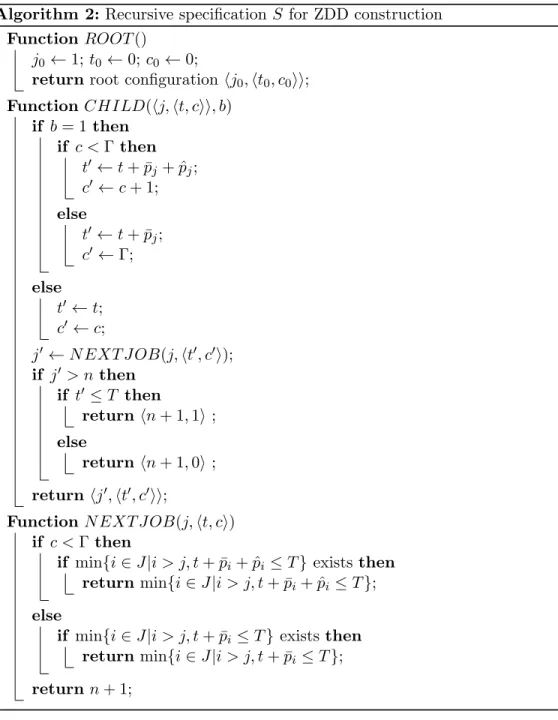
In this paper, in order to use the top-down construction framework, the recursive specification is specialized and redesigned. The recursive specification for finding all reachable configurations in the construction process is given in Algorithm 2. The ROOT() function returns the configuration of the root node in the ZDD as h1,h0,0ii, which means the root node starts with job 1 at time 0 and without jobs at their worst-case duration. CHILD(hj,ht, cii, b) decides the configuration of the b-child of the node with configuration hj,ht, cii. It first updates the stateht0, c0i for the child node. The 1-edge leads to an addition of processing time, and whether the deviation ˆpj should be

counted in depends on the value of worst-case counter c. The 0-edge finds the 0-childwith botht and c unchanged. With state ht0, c0i updated, the function N EXT J OB(j,ht0, c0i) determines the nearest next feasible jobj0 that can be appended to the current path towards the 1-terminalnode. If no job can still be appended, either the 1-terminalor the 0-terminalnode can be found based on the current feasibility condition.

Algorithm 2:Recursive specificationS for ZDD construction

Function ROOT()

j0 ←1;t0 ←0; c0←0;

returnroot configuration hj0,ht0, c0ii;

Function CHILD(hj,ht, cii, b) if b= 1 then if c <Γthen t0←t+ ¯pj+ ˆpj; c0 ←c+ 1; else t0←t+ ¯pj; c0 ←Γ; else t0←t; c0 ←c; j0 ←N EXT J OB(j,ht0, c0i); if j0 > n then if t0 ≤T then return hn+ 1,1i ; else return hn+ 1,0i ; returnhj0,ht0, c0ii;

Function N EXT J OB(j,ht, ci)

if c <Γthen

if min{i∈J|i > j, t+ ¯pi+ ˆpi ≤T} existsthen

return min{i∈J|i > j, t+ ¯pi+ ˆpi≤T};

else

if min{i∈J|i > j, t+ ¯pi≤T} existsthen

return min{i∈J|i > j, t+ ¯pi≤T};

returnn+ 1;

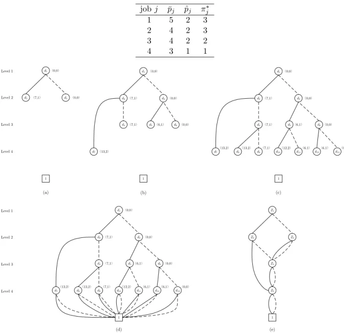
Figure 2 illustrates the construction process for a ZDD on a four-job example instance with Γ = 2 and T = 16. Detailed data for the example instance are given in Table 1. In Figure 2, the levels in the ZDD are indicated on the left, and the state of each node is shown in the label. All 1-edges are drawn in solid lines while the 0-edges appear as dotted lines. In Figure 2(a) the DD is initialized and the 1-child and 0-child at level 2 are identified. In Figure 2(b), all the children of the nodes at level 2 are then configured. It can be seen that the 1-edge of d2 skips level 3.

Table 1: A four-job instance with Γ = 2 andT = 16. job j p¯j pˆj πj∗ 1 5 2 3 2 4 2 3 3 4 2 2 4 3 1 1 d1 1 d2 d3 d1 1 d4 d2 d3 d7 d5 d6 〈0,0〉 d1 1 d4 d2 d3 d7 d5 d6 d8 d9 d10 d11 d12 d13 〈7,1〉 〈0,0〉 〈7,1〉 〈0,0〉 〈0,0〉 〈13,2〉 〈7,1〉 〈6,1〉 〈0,0〉 〈0,0〉 〈7,1〉 〈0,0〉 〈7,1〉 〈6,1〉 〈0,0〉 〈13,2〉 〈13,2〉 〈7,1〉 〈12,2〉 〈6,1〉 〈6,1〉 〈0,0〉 d1 1 d4 d2 d3 d7 d5 d6 d8 d9 d10 d11 d12 d13 〈0,0〉 〈7,1〉 〈0,0〉 〈7,1〉 〈6,1〉 〈0,0〉 〈13,2〉 〈13,2〉 〈7,1〉 〈12,2〉 〈6,1〉 〈6,1〉 〈0,0〉 Z1 1 Z4 Z2 Z3 Z5 (a) (b) (c) (d) (e) Level 2 Level 1 Level 3 Level 4 Level 2 Level 1 Level 3 Level 4

Figure 2: The ZDD construction process for the example instance

0-terminal, as job set{1,2,3}is not a feasible job group. Thusd2’s 1-childat level 3 is eliminated

automatically; this directly follows the reduction rule of ZDDs. In Figure 2(c), the children of the nodes at level 3 are determined, and then all feasible paths are made to terminate in the 1-terminal in Figure 2(d). After the construction of the DD, the reduction process is applied and the ZDD in Figure 2(e) is obtained. Each path from the root to the 1-terminal in the ZDD represents a feasible solution for the pricing problem, so once the ZDD for a node in the B&P tree is created we simply identify a longest path with the dual prices from the master as the lengths for the 1-edges. In this

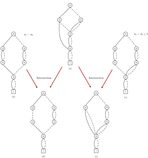
Z3 Z4 Z2 Z1 1 Z5 (e) Z3 Z5 Z2 Z4 Z1 1 Z6 (b) a1 = a3 Z1 1 Z4 Z2 Z3 Z5 (a) Intersection Intersection Z3 Z5 Z2 Z4 Z1 1 Z6 (c) a1 + a3 1 Z3 Z5 Z2 Z4 Z1 1 Z6 (d)

Figure 3: Construction of the ZDDs for the child nodes in the example instance (branch on jobs 1 and 3)

example the optimal objective value is 7, achieved by the job group {1,2,4}.

5.3 Branching with ZDDs

Upon branching in the B&P tree, new constraints are to be imposed in the pricing problems following the branching rule of Ryan and Foster (1981). The branching constraints need to be reflected in the ZDD structure of the child nodes; this be efficiently achieved by using the generic intersection operation for ZDDs. Figure 3 illustrates this process. Figure 3(a) contains the ZDD in the root node for the example instance, which contains all feasible solutions. We illustrate branching on jobs 1 and 3. Figure 3(b) depicts the ZDD containing all job combinations with only constraint a1 = a3 imposed. Similarly, the ZDD in Figure 3(c) represents the set of all job

ZDD with constraint a1 =a3 is then obtained in Figure 3(d). The intersection of Figure 3(a) and

Figure 3(c) represents all feasible job groups with a1+a3 ≤1, which is given in Figure 3(e).

In our experiments, we adopt the implementation choices of Kowalczyk and Leus (2016) to impose the branching constraints to the ZDDs of the non-root nodes in the B&P tree. In order avoid drastic changes to the structure of ZDDs and to keep the number of nodes in the ZDDs manageable, job pairs with close job indices are preferably chosen for branching: among all job pairs that can be branched after acquiring the non-integral LP solution, a pairj, j0 with the smallest difference|j−j0|is selected.

6

Computational experiments

6.1 Experimental setup

All algorithms are implemented in Visual C++. The computational experiments are performed on a PC equipped with Intel Core i7-4790 CPU at 3.6 GHz with 8 GB of RAM on a Windows 10 64-bit OS. All LPs and MIPs are solved with CPLEX 12.6.3 using Concert Technology with default settings. The algorithms are tested on a diverse set of instances, which are generated randomly as follows. The number of jobs n is either 30, 60, 90, 120 or 150 (below also referred to as instance size). The processing times are integers uniformly drawn from interval [1,20] or [1,100] (below referred to as p-range). The processing-time deviation is 0.2 times the processing time, rounded to the nearest higher integer. Five robustness levels are considered by varying Γ = dγne with γ either 0%, 5%, 10%, 15% or 20%. Four deadlines are generated for each instance, which are equal to a fraction frac of the sum of the worst-case job processing times; we examine frac= 1/4, 1/6, 1/8 and 1/10. For each combination of parameter settings, 10 instances are randomly generated, which leads to a set of 5×2×5×4×10 = 2000 instances in total. The time limit for each run of the algorithms on one instance is 1200 seconds (20 minutes).

6.2 Computational results

In the tables, the entries foropt show the number of instances solved to optimality within the time limit, out of 10 instances per setting. Columns labeled by time contain the average CPU time in seconds. We first show the results of the intuitive formulation (5) for instances of size 30 in

Table 2: Computational results of the intuitive formulation on instances withn= 30 p-range[1, 20] p-range[1, 100]

γ frac opt time opt time

0% 1/4 10 0.07 10 0.06 1/6 10 0.07 10 0.08 1/8 10 0.06 10 0.06 1/10 10 0.06 10 0.06 5% 1/4 10 0.28 10 0.28 1/6 10 0.45 10 0.40 1/8 10 1.39 10 1.16 1/10 10 122.63 10 4.70 10% 1/4 10 0.32 10 0.33 1/6 10 0.45 10 0.76 1/8 10 1.58 10 2.36 1/10 4 723.38 4 751.91 15% 1/4 10 0.40 10 0.58 1/6 10 1.20 10 2.50 1/8 3 845.62 5 676.35 1/10 4 859.89 0 1200.00 20% 1/4 10 0.65 10 0.80 1/6 10 1.34 10 128.75 1/8 2 1002.89 2 986.60 1/10 2 962.08 0 1200.00 Overall 165 226.24 161 247.89

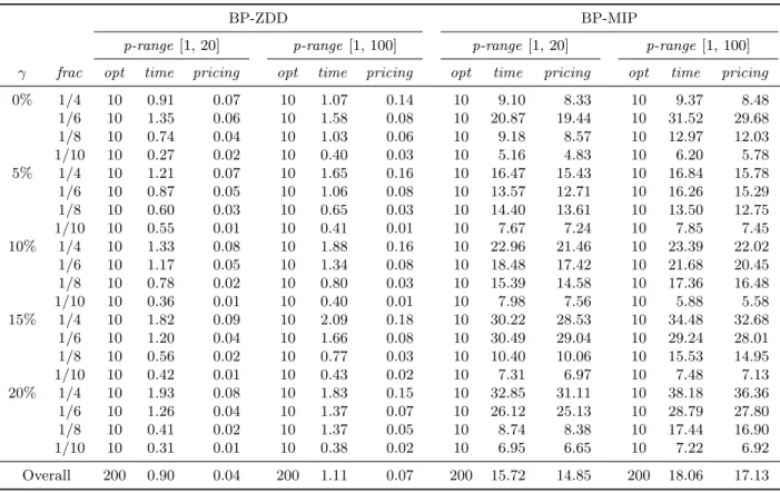
Table 3: Computational results of the two B&P algorithms on instances with n= 30

BP-ZDD BP-MIP

p-range[1, 20] p-range[1, 100] p-range[1, 20] p-range [1, 100]

γ frac opt time pricing opt time pricing opt time pricing opt time pricing

0% 1/4 10 0.91 0.07 10 1.07 0.14 10 9.10 8.33 10 9.37 8.48 1/6 10 1.35 0.06 10 1.58 0.08 10 20.87 19.44 10 31.52 29.68 1/8 10 0.74 0.04 10 1.03 0.06 10 9.18 8.57 10 12.97 12.03 1/10 10 0.27 0.02 10 0.40 0.03 10 5.16 4.83 10 6.20 5.78 5% 1/4 10 1.21 0.07 10 1.65 0.16 10 16.47 15.43 10 16.84 15.78 1/6 10 0.87 0.05 10 1.06 0.08 10 13.57 12.71 10 16.26 15.29 1/8 10 0.60 0.03 10 0.65 0.03 10 14.40 13.61 10 13.50 12.75 1/10 10 0.55 0.01 10 0.41 0.01 10 7.67 7.24 10 7.85 7.45 10% 1/4 10 1.33 0.08 10 1.88 0.16 10 22.96 21.46 10 23.39 22.02 1/6 10 1.17 0.05 10 1.34 0.08 10 18.48 17.42 10 21.68 20.45 1/8 10 0.78 0.02 10 0.80 0.03 10 15.39 14.58 10 17.36 16.48 1/10 10 0.36 0.01 10 0.40 0.01 10 7.98 7.56 10 5.88 5.58 15% 1/4 10 1.82 0.09 10 2.09 0.18 10 30.22 28.53 10 34.48 32.68 1/6 10 1.20 0.04 10 1.66 0.08 10 30.49 29.04 10 29.24 28.01 1/8 10 0.56 0.02 10 0.77 0.03 10 10.40 10.06 10 15.53 14.95 1/10 10 0.42 0.01 10 0.43 0.02 10 7.31 6.97 10 7.48 7.13 20% 1/4 10 1.93 0.08 10 1.83 0.15 10 32.85 31.11 10 38.18 36.36 1/6 10 1.26 0.04 10 1.37 0.07 10 26.12 25.13 10 28.79 27.80 1/8 10 0.41 0.02 10 1.37 0.05 10 8.74 8.38 10 17.44 16.90 1/10 10 0.31 0.01 10 0.38 0.02 10 6.95 6.65 10 7.22 6.92 Overall 200 0.90 0.04 200 1.11 0.07 200 15.72 14.85 200 18.06 17.13

Table 4: Computational results of the two B&P algorithms on instances with n= 60

BP-ZDD BP-MIP

p-range[1, 20] p-range[1, 100] p-range[1, 20] p-range[1, 100]

γ frac opt time pricing opt time pricing opt time pricing opt time pricing

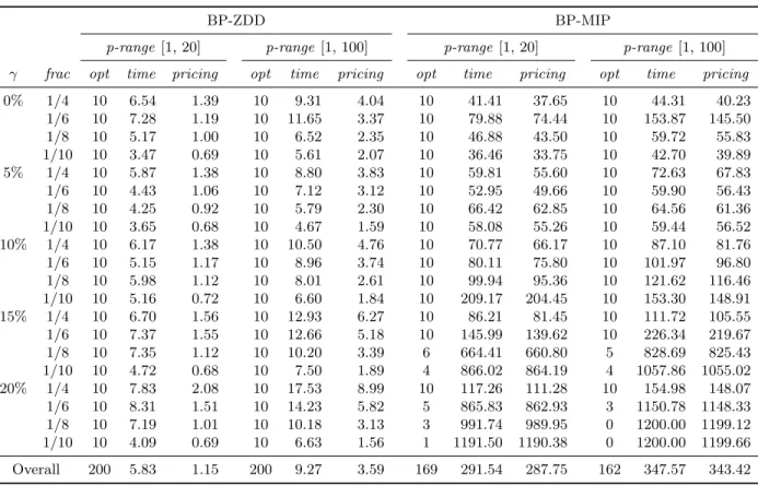
0% 1/4 10 6.54 1.39 10 9.31 4.04 10 41.41 37.65 10 44.31 40.23 1/6 10 7.28 1.19 10 11.65 3.37 10 79.88 74.44 10 153.87 145.50 1/8 10 5.17 1.00 10 6.52 2.35 10 46.88 43.50 10 59.72 55.83 1/10 10 3.47 0.69 10 5.61 2.07 10 36.46 33.75 10 42.70 39.89 5% 1/4 10 5.87 1.38 10 8.80 3.83 10 59.81 55.60 10 72.63 67.83 1/6 10 4.43 1.06 10 7.12 3.12 10 52.95 49.66 10 59.90 56.43 1/8 10 4.25 0.92 10 5.79 2.30 10 66.42 62.85 10 64.56 61.36 1/10 10 3.65 0.68 10 4.67 1.59 10 58.08 55.26 10 59.44 56.52 10% 1/4 10 6.17 1.38 10 10.50 4.76 10 70.77 66.17 10 87.10 81.76 1/6 10 5.15 1.17 10 8.96 3.74 10 80.11 75.80 10 101.97 96.80 1/8 10 5.98 1.12 10 8.01 2.61 10 99.94 95.36 10 121.62 116.46 1/10 10 5.16 0.72 10 6.60 1.84 10 209.17 204.45 10 153.30 148.91 15% 1/4 10 6.70 1.56 10 12.93 6.27 10 86.21 81.45 10 111.72 105.55 1/6 10 7.37 1.55 10 12.66 5.18 10 145.99 139.62 10 226.34 219.67 1/8 10 7.35 1.12 10 10.20 3.39 6 664.41 660.80 5 828.69 825.43 1/10 10 4.72 0.68 10 7.50 1.89 4 866.02 864.19 4 1057.86 1055.02 20% 1/4 10 7.83 2.08 10 17.53 8.99 10 117.26 111.28 10 154.98 148.07 1/6 10 8.31 1.51 10 14.23 5.82 5 865.83 862.93 3 1150.78 1148.33 1/8 10 7.19 1.01 10 10.18 3.13 3 991.74 989.95 0 1200.00 1199.12 1/10 10 4.09 0.69 10 6.63 1.56 1 1191.50 1190.38 0 1200.00 1199.66 Overall 200 5.83 1.15 200 9.27 3.59 169 291.54 287.75 162 347.57 343.42

Table 5: Computational results of the two B&P algorithms on instances with n= 90

BP-ZDD BP-MIP

p-range[1, 20] p-range[1, 100] p-range[1, 20] p-range[1, 100]

γ frac opt time pricing opt time pricing opt time pricing opt time pricing

0% 1/4 10 20.83 7.13 10 35.13 22.50 10 123.40 112.37 10 114.83 103.22 1/6 10 20.12 6.77 10 48.90 25.23 10 148.51 138.93 10 325.69 305.53 1/8 10 14.16 5.60 10 29.23 18.73 10 98.06 90.79 10 111.48 103.51 1/10 10 11.87 4.71 10 23.19 14.72 10 77.27 71.64 10 90.76 84.24 5% 1/4 10 21.48 7.78 10 42.11 27.28 10 158.04 146.18 10 165.15 153.06 1/6 10 16.15 7.34 10 32.83 23.63 10 119.95 112.67 10 129.59 121.91 1/8 10 14.42 6.11 10 28.50 19.16 10 178.53 171.71 10 166.89 159.15 1/10 10 13.46 5.22 10 23.26 14.29 10 283.37 276.72 10 204.43 196.89 10% 1/4 10 25.61 10.57 10 43.37 29.64 10 175.81 163.43 10 180.42 168.65 1/6 10 20.99 10.86 10 47.82 34.79 10 191.85 182.80 10 225.12 214.88 1/8 10 24.81 11.06 10 45.45 30.51 10 314.02 302.17 9 418.58 408.08 1/10 10 25.06 9.41 10 40.32 23.47 8 619.60 608.35 5 912.36 904.10 15% 1/4 10 31.52 15.87 10 73.95 56.08 9 314.41 302.12 10 293.92 277.05 1/6 10 41.28 21.00 10 81.78 57.57 10 395.27 379.04 4 1028.83 1021.92 1/8 10 37.84 15.31 10 54.95 34.84 1 1178.22 1176.47 0 1200.00 1199.53 1/10 10 31.69 12.57 10 44.07 27.09 0 1200.00 1199.62 0 1200.00 1199.51 20% 1/4 10 43.25 26.85 10 106.13 86.10 10 284.13 268.64 10 394.19 375.31 1/6 10 49.19 26.20 10 85.89 62.54 0 1200.00 1199.64 0 1200.00 1199.58 1/8 10 39.46 19.04 10 64.05 41.84 0 1200.00 1199.73 0 1200.00 1199.64 1/10 10 36.05 18.50 10 53.00 33.92 0 1200.00 1199.67 0 1200.00 1199.66 Overall 200 26.96 12.40 200 50.20 34.20 148 473.02 465.13 138 538.11 529.77

Table 6: Computational results of the two B&P algorithms on instances with n= 120

BP-ZDD BP-MIP

p-range[1, 20] p-range[1, 100] p-range[1, 20] p-range[1, 100]

γ frac opt time pricing opt time pricing opt time pricing opt time pricing

0% 1/4 10 46.53 22.52 10 110.49 84.45 10 198.06 178.13 10 196.04 173.64 1/6 10 45.18 23.37 10 131.71 92.07 10 264.59 245.20 10 522.65 487.14 1/8 10 32.37 19.61 10 92.64 77.43 10 151.77 140.76 10 187.11 173.39 1/10 10 26.67 16.23 10 82.25 69.33 10 128.86 119.10 10 150.62 139.62 5% 1/4 10 59.80 34.03 10 122.19 95.69 10 242.77 221.96 10 249.59 228.55 1/6 10 49.21 35.58 10 111.00 96.80 10 191.92 180.00 10 198.40 186.32 1/8 10 45.83 31.70 10 92.89 79.87 0 1200.00 1198.89 10 448.60 436.73 1/10 10 44.27 30.17 10 85.75 71.95 0 1200.00 1199.42 5 1001.39 994.70 10% 1/4 10 79.40 50.77 10 150.20 124.36 10 288.28 264.71 10 318.59 293.93 1/6 10 80.27 63.27 10 192.73 172.84 10 590.56 575.17 7 663.14 650.24 1/8 10 81.27 61.00 10 190.52 163.42 2 1121.00 1112.07 1 1187.96 1182.99 1/10 10 103.90 72.59 10 168.48 136.82 0 1200.00 1199.44 0 1200.00 1199.50 15% 1/4 10 63.56 35.64 10 219.72 190.87 9 408.42 386.53 10 424.50 397.40 1/6 10 80.48 52.08 10 289.97 251.38 8 755.99 732.60 3 1097.80 1073.34 1/8 10 64.37 28.07 10 192.31 151.61 1 1139.44 1137.46 0 1200.00 1199.44 1/10 10 65.08 25.41 10 138.91 101.48 0 1200.00 1199.50 0 1200.00 1199.56 20% 1/4 10 83.32 57.07 10 336.67 300.37 10 449.94 422.62 10 655.45 620.39 1/6 10 92.11 48.44 10 281.49 233.40 0 1200.00 1199.60 0 1200.00 1199.44 1/8 10 58.05 24.77 10 170.46 126.25 1 1191.05 1190.24 0 1200.00 1199.53 1/10 10 56.43 19.38 10 121.02 84.72 0 1200.00 1199.51 0 1200.00 1199.63 Overall 200 62.91 37.58 200 164.07 135.26 111 716.13 705.15 116 725.09 711.77

Table 7: Computational results of the two B&P algorithms on instances with n= 150

BP-ZDD BP-MIP

p-range[1, 20] p-range[1, 100] p-range[1, 20] p-range[1, 100]

γ frac opt time pricing opt time pricing opt time pricing opt time pricing

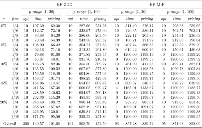
0% 1/4 10 107.39 62.30 10 287.66 234.28 10 311.40 276.17 10 298.58 259.65 1/6 10 112.37 72.19 10 338.97 273.99 10 420.35 386.11 10 762.51 703.91 1/8 10 83.88 64.29 10 286.60 263.50 10 222.17 205.83 10 254.91 236.39 1/10 10 70.49 54.39 10 243.58 225.52 10 186.21 171.92 10 212.08 196.64 5% 1/4 10 108.90 66.42 10 304.21 257.63 10 407.44 366.83 10 422.32 379.29 1/6 10 92.16 71.10 10 312.32 291.80 9 619.42 600.49 10 450.61 430.63 1/8 10 79.88 61.00 10 271.83 253.45 0 1200.00 1199.19 0 1200.00 1199.29 1/10 10 65.87 48.01 10 231.76 210.47 0 1200.00 1199.53 0 1200.00 1199.32 10% 1/4 10 136.78 82.36 10 355.50 309.27 10 461.99 417.68 10 422.41 382.01 1/6 10 135.55 109.52 10 607.62 577.89 0 1200.00 1198.58 6 1020.78 1005.84 1/8 10 153.56 118.49 10 604.86 557.04 0 1200.00 1199.25 0 1200.00 1199.33 1/10 10 156.47 101.74 10 498.29 429.09 0 1200.00 1199.14 0 1200.00 1199.36 15% 1/4 10 164.96 114.57 10 654.63 602.49 10 600.37 546.83 9 676.27 630.98 1/6 10 211.56 167.38 10 1006.05 929.47 4 1165.01 1133.67 0 1200.00 1188.77 1/8 10 228.59 140.63 10 654.97 560.18 0 1200.00 1199.12 0 1200.00 1199.43 1/10 10 202.36 115.29 10 485.35 393.37 0 1200.00 1199.07 0 1200.00 1199.50 20% 1/4 10 243.43 188.72 4 980.14 935.49 9 859.23 805.61 10 912.05 853.43 1/6 10 238.39 157.62 10 1052.19 951.14 1 1092.01 1091.07 0 1200.00 1199.30 1/8 10 226.95 130.01 10 639.81 542.12 0 1200.00 1199.22 0 1200.00 1199.38 1/10 10 171.78 95.56 10 359.53 251.86 0 1200.00 1199.10 0 1200.00 1199.35 Overall 200 149.57 101.08 194 508.79 452.50 93 857.28 839.72 95 871.63 853.09

Table 2. Clearly, the intuitive formulation already struggles with these small instances, especially with relatively large Γ values and shorter deadlines. For instances of size 30, the intuitive formu-lation already fails to solve 74 out of 400 instances, and its overall run time is orders of magnitude higher than for the B&P algorithms reported below. Due to this poor computational performance, we will not further include this formulation in the comparison for larger instances.

Two B&P algorithms are implemented and compared. The global routine is the same, the difference resides in the pricing solver. We denote the B&P algorithm with the ZDD-based pricing solver as BP-ZDD, while BP-MIP refers to the use of MIP-solver for formulation (9) for pricing. In BP-ZDD the branching constraints are imposed on the ZDDs as described in Section 5.3, while in MIP they are added to formulation (9). The computational comparison of ZDD and BP-MIP is summarized in Tables 3 to 7. Since both B&P algorithms follow the same overall routine and differ only in the pricing method, the average run time spent on the pricing procedures is included separately in the columns labeledpricing (in seconds).

Overall, BP-ZDD yields a consistently better performance than BP-MIP, solving all instances from size 30 to size 120 and only failing to solve six instances with size 150. BP-MIP solves all instances with n = 30 within the time limit, but already starts to experience difficulties for size 60. The performance gradually worsens with increasingn, with less than half of the instances with n = 150 solved to guaranteed optimality. The reason why BP-ZDD fails on six instances is because the size of ZDDs becomes very large, with number of nodes close to one million, thus the construction of ZDDs and branching are no longer easy to handle and it takes longer to trace a longest path in those ZDDs. When BP-MIP fails, it usually gets stuck with a pricing problem. The benefit of applying ZDDs for pricing is obvious in the smaller instances (n= 30 and 60): the average run time for pricing in BP-ZDD is lower than BP-MIP by roughly two orders of magnitude. For larger instances, the actual difference in run times cannot be accurately measured as BP-MIP failed for many instances, but it is clear that BP-ZDD achieves a superior performance thanks to its more efficient pricing solver.

The value of Γ significantly influences the difficulty of the instances. For both algorithms, the larger the Γ value, the longer it takes for an algorithm to solve an instance. For BP-MIP, the number of solved instances clearly decreases as the value of Γ grows, and so the consideration of robustness, which is reflected in Γ, is one of the main factors of difficulty of an instance.

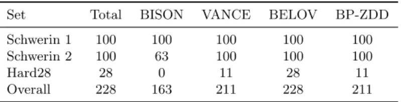
Table 8: Number of the BPP instances solved by different methods in less than one minute

Set Total BISON VANCE BELOV BP-ZDD Schwerin 1 100 100 100 100 100 Schwerin 2 100 63 100 100 100

Hard28 28 0 11 28 11

Overall 228 163 211 228 211

BP-ZDD and BP-MIP have a very different dependence on the deadline. As mentioned before, the pricing problem is a robust variant of the knapsack problem. Since a larger deadline means that more jobs can be assigned to one individual machine, this increases the difficulty in BP-ZDD due to the larger ZDDs, with longer paths and more nodes, which explains why BP-ZDD cannot solve all instances in Table 7 with the largest Γ and highestfrac. For BP-MIP exactly the opposite occurs: it can still solve most of the instances with high frac but struggles with lower frac. This phenomenon goes against the trend for knapsack problems; one possible reason is that the extra constraints and variables in formulation (9) significantly change its structure compared to a general knapsack problem.

The different ranges of processing times do not have much impact on the CPU time and the number of solved instances for BP-MIP. For BP-ZDD, by contrast, a wider range coincides with more states in the ZDDs, which increases the size of the ZDDs and makes the manipulation of ZDDs less efficient. Tables 3 to 7 show that the average pricing time for range [1,20] is only a fraction of the results for the wider range [1,100] for BP-ZDD, and its average run time in any setting with time range [1,20] never exceeds 250 seconds.

6.3 Results for bin packing instances

The deterministic variant of RMAP coincides with the classic bin packing problem BPP. Since our procedure solves a more general problem variant, it can also solve the conventional BPP. In order to validate the performance of our method, we therefore also test on some benchmark BPP instances, and compare with several dedicated approaches for the BPP. We have selected three instances sets for BPP, namely the sets “Schwerin 1” and “Schwerin 2” from Schwerin and W¨ascher (1997), with 100 instances both for n= 100 and for 120, and set “Hard28”, which contains 28 hard instances from Schoenfield (2002), with sizes from 160 to 200. The data are obtained from BPPLIB1.

1

Three dedicated methods for BPP are chosen for comparison, which are the well-known B&B algorithm BISON from Scholl et al. (1997), the classic B&P algorithm proposed by Vance et al. (1994), denoted as VANCE, which also uses the Ryan and Foster branching rule, and the branch-and-cut-and-price algorithm by Belov and Scheithauer (2006), denoted as BELOV. The computa-tional results for these benchmark algorithms are taken from the latest BPP review by Delorme et al. (2016), where the experiments are executed on a quad-core Intel Xeon CPU at 3.10 GHz with 8 GB RAM using only one thread on one core.

For BP-ZDD, we simply set Γ and the processing-time deviations to zero, and we set the number of threads that can be used as one. The results of the four methods on the three instance sets are reported in Table 8 for a time limit of one minute. It can be seen that BP-ZDD solves more instances than BISON in the same time period, while it equalizes the performance of VANCE, which uses the same overall routine. For the set Hard28, the state-of-the-art BELOV algorithm is able to find guaranteed optimal solutions to more instances, however. BELOV has the advantage of generating additional constraints to cut off non-integral solutions. We have not applied such enhancements in our procedure, because the generated cuts and the dual variables entailed by the cuts generally invalidate DP for the pricing problem (Belov and Scheithauer, 2006), while we see no efficient implicit enumeration method that could solve the corresponding pricing problem in RMAP (Belov and Scheithauer, 2006, use B&B for their pricing problem). Since the procedure BP-ZDD has been developed for a more general problem setting, we conclude that it has an adequate competitive performance on the conventional BPP instances.

6.4 Sensitivity analysis

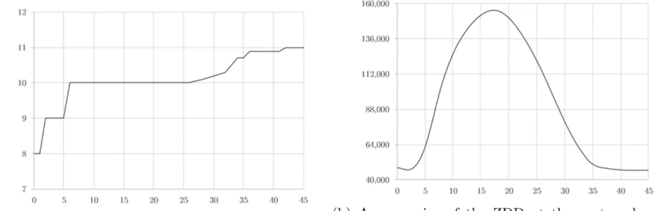
The budget of uncertainty Γ is the key parameter of our model. In this section we examine its influence on the optimal objective value, and following up on our discussion in Section 6.2 we also zoom in on the impact of Γ on the difficulty of the instances, for which the size of the ZDD at the root node is a direct reflection. We generate 10 instances of 120 jobs, fixing the duration deviations at 30% of the processing times (rounded to the higher integer), and frac= 1/10. For a wide range of Γ values, we compute the average objective value (number of machines) and the size of the ZDD at the root node. The results are shown in Figure 4.

non-(a) Average number of machines as a function of Γ (b) Average size of the ZDD at the root node as a function of Γ

Figure 4: The impact of Γ on the objective value and on the difficulty of the instances

decreasing overall, as more machines or higher cost will be incurred to guarantee a stronger ro-bustness. The curve starts at Γ = 0 (no protection provided), where eight machines are needed on average. The curve reaches its maximum value of 11 at Γ = 42, and any Γ≥42 simply corresponds to the same worst case. The curve displays several plateaus, which is a consequence of the slack-ness provided in the gap between the optimal LP and integral solution. Within these plateaus, the objective value is insensitive to Γ, where a relatively larger Γ could be chosen for higher robustness. Figure 4(b) plots the average size of the root-node ZDD as a function of Γ; a bell-shaped pattern occurs. In the left part of the graph, the average size climbs with increasing Γ, reaching a peak at around 155,000 for Γ = 18. Here, larger Γ results in more states in the ZDDs, and generates more unique paths with non-equivalent nodes that can not be suppressed. As Γ increases beyond value 18, the plot goes down again, because more jobs are forced to take on their worst-case duration along each path, and thus more similar paths are generated with more equivalent nodes that can be merged in the ZDDs. When Γ reaches a critical value where all jobs are forced into their worst-case duration, the size of the ZDD no longer changes with increasing Γ. At the two ends of the curve, the average sizes of the ZDDs are very close to each other, which is not unlogical: both Γ values essentially represent deterministic cases, either the nominal case or the worst case.

7

Conclusions

In this work, we have considered a time-driven scheduling problem in a parallel machine environ-ment, which we have entitled the machine availability problem, which minimizes the number of identical machines that are necessary to complete the job set before a given deadline. We have studied this problem in a context of uncertainty, leading to the robust machine availability problem RMAP, which uses an uncertainty set for the job durations following Bertsimas and Sim (2004), with a budget of uncertainty limiting the number of deviating job durations.

An intuitive formulation for RMAP is presented, followed by a set covering formulation and a B&P procedure for better computational performance. We introduce ZDDs for solving the pricing problem to tackle the difficulty entailed by the robustness considerations and by the extra con-straints imposed by branching decisions. Two B&P algorithms are tested and compared, where pricing is done using ZDDs and using a generic MIP solver, respectively. Our computational results show that the B&P algorithm with ZDDs has superior performance. Experiments on classic bin packing instances confirm the adequate functioning of the proposed algorithm.

Further research in this area may include the study of different objective functions, such as makespan minimization or the sum of weighted completion times; to this respect, it should be noted that the current paper also contributes to the development of a solution method for a corresponding robust variant of P||Cmax, which could be solved using RMAP as a subproblem in a binary search

procedure, similarly to Dell’Amico et al. (2008). Other opportunities for studying richer scheduling models are legion, such as the introduction of precedence constraints or the inclusion of multiple resource categories.

References

Akers, S. B. (1978). Binary decision diagrams. IEEE Transactions on Computers, 27(6):509–516. Belov, G. and Scheithauer, G. (2006). A branch-and-cut-and-price algorithm for one-dimensional

stock cutting and two-dimensional two-stage cutting. European Journal of Operational Research, 171(1):85–106.

Ben-Tal, A., Goryashko, A., Guslitzer, E., and Nemirovski, A. (2004). Adjustable robust solutions of uncertain linear programs. Mathematical Programming, 99(2):351–376.

Ben-Tal, A. and Nemirovski, A. (1998). Robust convex optimization. Mathematics of Operations Research, 23(4):769–805.

Ben-Tal, A. and Nemirovski, A. (1999). Robust solutions of uncertain linear programs. Operations Research Letters, 25(1):1–13.

Ben-Tal, A. and Nemirovski, A. (2000). Robust solutions of linear programming problems contam-inated with uncertain data. Mathematical Programming, 88(3):411–424.

Bergman, D., Cire, A. A., van Hoeve, W.-J., and Hooker, J. N. (2016). Discrete optimization with decision diagrams. INFORMS Journal on Computing, 28(1):47–66.

Bertsimas, D., Pachamanova, D., and Sim, M. (2004). Robust linear optimization under general norms. Operations Research Letters, 32(6):510–516.

Bertsimas, D. and Sim, M. (2003). Robust discrete optimization and network flows. Mathematical Programming, 98(1-3):49–71.

Bertsimas, D. and Sim, M. (2004). The price of robustness. Operations Research, 52(1):35–53. Bougeret, M., Pessoa, A. A., and Poss, M. (2016). Robust scheduling with budgeted uncertainty.

HAL, open archives, hal-01345283. https://hal.archives-ouvertes.fr/hal-01345283.

Brand˜ao, F. and Pedroso, J. P. (2016). Bin packing and related problems: General arc-flow formu-lation with graph compression. Computers & Operations Research, 69:56–67.

Charnes, A. and Cooper, W. W. (1959). Chance-constrained programming. Management Science, 6(1):73–79.

Chopra, S. and Meindl, P. (2013). Supply Chain Management: Strategy, Planning, And Operation. Pearson.

Coughlan, E. T., L¨ubbecke, M. E., and Schulz, J. (2015). A branch-price-and-cut algorithm for multi-mode resource leveling. European Journal of Operational Research, 245(1):70–80.

Daniels, R. L. and Kouvelis, P. (1995). Robust scheduling to hedge against processing time uncer-tainty in single-stage production. Management Science, 41(2):363–376.

Dantzig, G. B. (1955). Linear programming under uncertainty. Management Science, 1(3-4):197– 206.

De Carvalho, J. V. (1999). Exact solution of bin-packing problems using column generation and branch-and-bound. Annals of Operations Research, 86:629–659.

De Carvalho, J. V. (2002). LP models for bin packing and cutting stock problems. European Journal of Operational Research, 141(2):253–273.

Degraeve, Z. and Peeters, M. (2003). Optimal integer solutions to industrial cutting-stock problems: Part 2, benchmark results. INFORMS Journal on Computing, 15(1):58–81.

Degraeve, Z. and Schrage, L. (1999). Optimal integer solutions to industrial cutting stock problems.

INFORMS Journal on Computing, 11(4):406–419.

Dell’Amico, M., Iori, M., Martello, S., and Monaci, M. (2008). Heuristic and exact algorithms for the identical parallel machine scheduling problem. INFORMS Journal on Computing, 20(3):333– 344.

Dell’Amico, M. and Martello, S. (1995). Optimal scheduling of tasks on identical parallel processors.

ORSA Journal on Computing, 7(2):191–200.

Dell’Amico, M. and Martello, S. (2005). A note on exact algorithms for the identical parallel machine scheduling problem. European Journal of Operational Research, 160(2):576–578. Delorme, M., Iori, M., and Martello, S. (2016). Bin packing and cutting stock problems:

Mathe-matical models and exact algorithms. European Journal of Operational Research, 255(1):1–20. Demeulemeester, E. (1995). Minimizing resource availability costs in time-limited project networks.

Management Science, 41(10):1590–1598.

Dyckhoff, H. (1981). A new linear programming approach to the cutting stock problem.Operations Research, 29(6):1092–1104.

Easa, S. M. (1989). Resource leveling in construction by optimization. Journal of Construction Engineering and Management, 115(2):302–316.

El Ghaoui, L. and Lebret, H. (1997). Robust solutions to least-squares problems with uncertain data. SIAM Journal on Matrix Analysis and Applications, 18(4):1035–1064.

El Ghaoui, L., Oustry, F., and Lebret, H. (1998). Robust solutions to uncertain semidefinite programs. SIAM Journal on Optimization, 9(1):33–52.

Farley, A. A. (1990). A note on bounding a class of linear programming problems, including cutting stock problems. Operations Research, 38(5):922–923.

Garey, M. R. and Johnson, D. S. (1979). Computers and Intractability: A Guide to the Theory of NP-completeness. W. H. Freeman and Company, New York.

Gilmore, P. C. and Gomory, R. E. (1961). A linear programming approach to the cutting-stock problem. Operations Research, 9(6):849–859.

Goren, S. and Sabuncuoglu, I. (2009). Optimization of schedule robustness and stability under random machine breakdowns and processing time variability. IIE Transactions, 42(3):203–220. Graves, S. C. (1981). A review of production scheduling. Operations Research, 29(4):646–675. Hans, E. (2001).Resource loading by branch-and-price techniques. PhD thesis, University of Twente,

The Netherlands.

Harris, R. B. (1990). Packing method for resource leveling (pack). Journal of Construction Engi-neering and Management, 116(2):331–350.

Herroelen, W. and Leus, R. (2005). Project scheduling under uncertainty: Survey and research potentials. European Journal of Operational Research, 165(2):289–306.

Hooker, J. N. (2013). Decision diagrams and dynamic programming. In International Conference on AI and OR Techniques in Constraint Programming for Combinatorial Optimization Problems, pages 94–110. Springer.

Iwashita, H. and Minato, S. (2013). Efficient top-down ZDD construction techniques using recur-sive specifications. TCS Technical reports TCS-TR-A-13-69, Hokkaido University, Division of Computer Science.

Janak, S. L., Lin, X., and Floudas, C. A. (2007). A new robust optimization approach for scheduling under uncertainty: II. Uncertainty with known probability distribution. Computers & Chemical Engineering, 31(3):171–195.

Knuth, D. (2009). The Art of Computer Programming, Volume 4, Fascicle 1: Bitwise Tricks & Techniques; Binary Decision Diagrams. Addison-Wesley Professional, 12th edition.

Kouvelis, P., Daniels, R. L., and Vairaktarakis, G. (2000). Robust scheduling of a two-machine flow shop with uncertain processing times. IIE Transactions, 32(5):421–432.

Kouvelis, P. and Yu, G. (1997). Robust Discrete Optimization and Its Applications. Kluwer, Dordrecht.

Kowalczyk, D. and Leus, R. (2016). A branch-and-price algorithm for parallel machine scheduling using ZDDs and generic branching. FEB Research Report KBI 1631, KU Leuven-Faculty of Economics and Business, Leuven, Belgium.

Lee, C.-Y. (1959). Representation of switching circuits by binary-decision programs. Bell Labs Technical Journal, 38(4):985–999.

Leon, J. V., Wu, D. S., and Storer, R. H. (1994). Robustness measures and robust scheduling for job shops. IIE Transactions, 26(5):32–43.

Leu, S.-S., Yang, C.-H., and Huang, J.-C. (2000). Resource leveling in construction by genetic algorithm-based optimization and its decision support system application. Automation in Con-struction, 10(1):27–41.

Leus, R. and Herroelen, W. (2004). Stability and resource allocation in project planning. IIE Transactions, 36(7):667–682.

under uncertainty: I. Bounded uncertainty. Computers & Chemical Engineering, 28(6):1069– 1085.

Lopes, M. J. P. and de Carvalho, J. V. (2007). A branch-and-price algorithm for scheduling parallel machines with sequence dependent setup times. European Journal of Operational Research, 176(3):1508–1527.

Martello, S. and Toth, P. (1990). Lower bounds and reduction procedures for the bin packing problem. Discrete Applied Mathematics, 28(1):59–70.

Minato, S. (1993). Zero-suppressed BDDs for set manipulation in combinatorial problems. In

Proceedings of the 30th international Design Automation Conference, pages 272–277. ACM. Minato, S. (2001). Zero-suppressed BDDs and their applications.International Journal on Software

Tools for Technology Transfer, 3(2):156–170.

M¨ohring, R. H. (1984). Minimizing costs of resource requirements in project networks subject to a fixed completion time. Operations Research, 32(1):89–120.

Mokotoff, E. (2004). An exact algorithm for the identical parallel machine scheduling problem.

European Journal of Operational Research, 152(3):758–769.

Morrison, D. R., Sewell, E. C., and Jacobson, S. H. (2016). Solving the pricing problem in a branch-and-price algorithm for graph coloring using zero-suppressed binary decision diagrams.

INFORMS Journal on Computing, 28(1):67–82.

Mula, J., Poler, R., Garcia-Sabater, J., and Lario, F. C. (2006). Models for production planning under uncertainty: A review. International Journal of Production Economics, 103(1):271–285. Pferschy, U. and Schauer, J. (2009). The knapsack problem with conflict graphs. Journal of Graph

Algorithms and Applications, 13(2):233–249.

Pinedo, M. (2015). Scheduling: Theory, Algorithms, and Systems. Springer, 5th edition.

Rodrigues, S. B. and Yamashita, D. S. (2010). An exact algorithm for minimizing resource avail-ability costs in project scheduling. European Journal of Operational Research, 206(3):562–568.

Ryan, D. M. and Foster, B. A. (1981). An integer programming approach to scheduling. Computer Scheduling of Public Transport Urban Passenger Vehicle and Crew Scheduling, pages 269–280. Schoenfield, J. E. (2002). Fast, exact solution of open bin packing problems without linear

program-ming. US Army Space and Missile Defense Command Technical Report, Huntsville, Alabama, USA.

Scholl, A., Klein, R., and J¨urgens, C. (1997). Bison: A fast hybrid procedure for exactly solving the one-dimensional bin packing problem. Computers & Operations Research, 24(7):627–645. Schwerin, P. and W¨ascher, G. (1997). The bin-packing problem: A problem generator and some

numerical experiments with ffd packing and mtp. International Transactions in Operational Research, 4(5-6):377–389.

Soyster, A. L. (1973). Convex programming with set-inclusive constraints and applications to inexact linear programming. Operations Research, 21(5):1154–1157.

van den Akker, J. M., Hoogeveen, J. A., and van de Velde, S. L. (1999). Parallel machine scheduling by column generation. Operations Research, 47(6):862–872.

Vance, P. H. (1998). Branch-and-price algorithms for the one-dimensional cutting stock problem.

Computational Optimization and Applications, 9(3):211–228.

Vance, P. H., Barnhart, C., Johnson, E. L., and Nemhauser, G. L. (1994). Solving binary cutting stock problems by column generation and branch-and-bound. Computational Optimization and Applications, 3(2):111–130.

Vanderbeck, F. (1999). Computational study of a column generation algorithm for bin packing and cutting stock problems. Mathematical Programming, 86(3):565–594.

Vanderbeck, F. (2000a). Exact algorithm for minimising the number of setups in the one-dimensional cutting stock problem. Operations Research, 48(6):915–926.

Vanderbeck, F. (2000b). On Dantzig-Wolfe decomposition in integer programming and ways to perform branching in a branch-and-price algorithm. Operations Research, 48(1):111–128.

Vanderbeck, F. (2011). Branching in branch-and-price: A generic scheme. Mathematical Program-ming, 130(2):249–294.

Wiest, J. D., Levy, F. K., et al. (1969). Management guide to PERT/CPM. NJ, Prentice-Hall. Wullink, G., Gademann, A., Hans, E. W., and van Harten, A. (2004). Scenario-based approach

for flexible resource loading under uncertainty. International Journal of Production Research, 42(24):5079–5098.

FACULTY OF ECONOMICS AND BUSINESS Naamsestraat 69 bus 3500 3000 LEUVEN, BELGIË tel. + 32 16 32 66 12 fax + 32 16 32 67 91 [email protected] www.econ.kuleuven.be