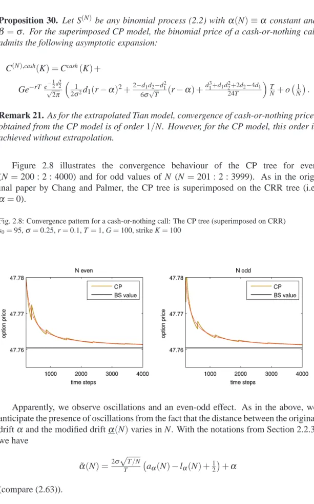
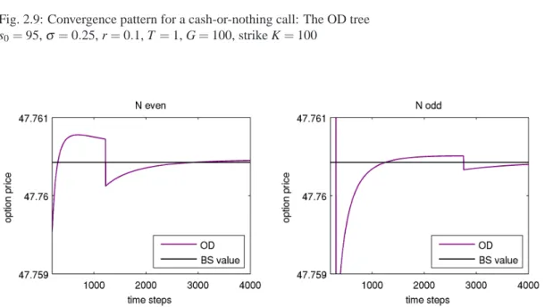
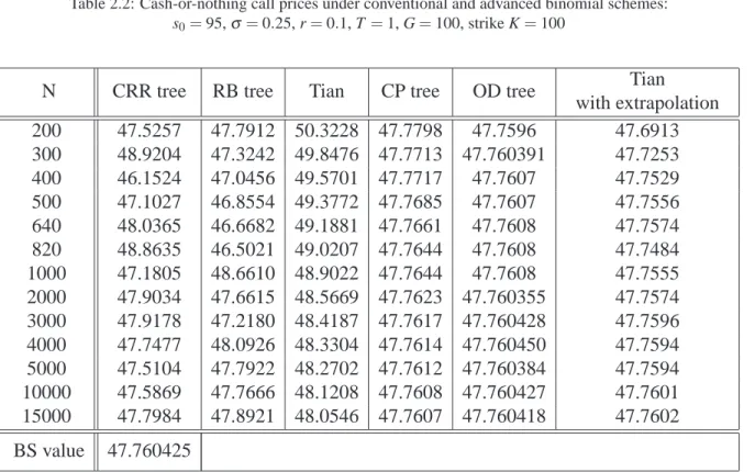
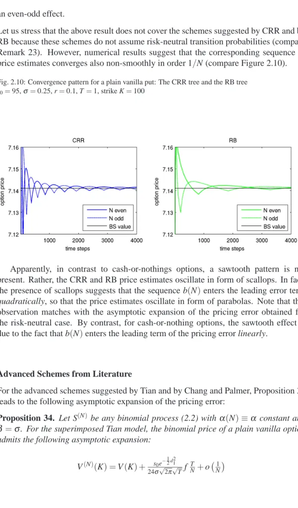
to Option Valuation
Getting Binomial Trees into Shape
Stefanie M ¨uller
1. Gutachter: Prof. Dr. Ralf Korn
2. Gutachter: Prof. L.C.G. Rogers, Ph.D. Datum der Disputation: 16. Dezember 2009
University of Kaiserslautern Erwin-Schr ¨odinger-Straße 67663 Kaiserslautern
to Option Valuation
Getting Binomial Trees into Shape
Stefanie M ¨uller
Vom Fachbereich Mathematik der Technischen Universit ¨at Kaiserslautern zur Verleihung des akademischen Grades Doktor der Naturwissenschaften (Doctor rerum naturalium, Dr. rer. nat.) genehmigte Dissertation.
1. Gutachter: Prof. Dr. Ralf Korn
2. Gutachter: Prof. L.C.G. Rogers, Ph.D.
Datum der Disputation: 16. Dezember 2009
First, I would like to express my deep gratitude to my supervisor, Prof. Dr. Ralf Korn. His support and advice were invaluable to me. I am especially grateful for his close co-operation while working on our joint papers.
I am also very grateful to Prof. Dr. Chris Rogers for accepting to act as a referee for this thesis and for his hospitality during my research visits to the Cambridge Statistical Laboratory. I benefited a lot from his feedback.
I deeply wish to thank Frank Seifried and my father Stefan M¨uller for their innumerable discussions with me. I very much appreciated their suggestions. Further, many thanks go to Dr. Kalina Natcheva-Acar. In my first year, Kalina kindly shared her valuable experiences in com-putational finance with me.
I would like to thank my colleagues and friends at the department and at the Fraunhofer ITWM; in particular, Dr. Peter Diesinger, Prof. Dr. J¨orn Sass and Nicole Tschauder; Dr. Matthias Fengler and Junior-prof. Dr. Natalie Packham for invitations to the Trading & Derivatives group of Sal. Oppenheim and to the Frankfurt School of Finance & Management; Prof. Dr. Mark Broadie and Dr. Mike Staunton for valu-able comments and software code; Prof. Dr. Wolfgang Runggaldier, whose AARMS summer course intensified my interest in research on mathematical finance.
Finally, I gratefully acknowledge the financial support of the Rheinland-Pfalz cluster of excellence DASMOD and the Center for Computational and Mathematical Modelling.
1 Introduction 1
2 Binomial Pricing for Single-Asset Options 7
2.1 Introduction . . . 7
2.2 Discretisation of the Stock Price and Weak Convergence . . . 8
2.2.1 Binomial Models . . . 9
2.2.2 Distributional Fit . . . 21
2.2.3 Advanced Binomial Models . . . 35
2.3 Convergence of Binomial Option Prices . . . 44
2.3.1 European-Type Options . . . 45
2.3.2 American-Type Options . . . 55
2.4 Tree Procedures . . . 57
2.4.1 Variants of the Tree Algorithm . . . 57
2.4.2 Connection to Explicit Finite Difference Methods . . . 67
2.5 The Convergence Behaviour of Binomial Option Prices . . . 73
2.5.1 Constant Payoff Structures (Cash-or-Nothing Options) . . . 75
2.5.2 Linear Payoff Structures (Plain Vanilla Options) . . . 92
2.6 Conclusion . . . 104
3 The Standard Approach to Multi-Dimensional Trees 105 3.1 Introduction . . . 105
3.3 Option Valuation with Standard Multi-Dimensional Trees . . . 112
3.3.1 The Tree Algorithm . . . 112
3.3.2 The Convergence Behaviour of Binomial Option Prices . . . 114
4 The Decoupling Approach to Multi-Dimensional Trees 123 4.1 Introduction . . . 123
4.2 A General Decoupling Method . . . 124
4.3 Discretisation of the Decoupled Process and Backtransformation . . . . 130
4.4 Binomial Option Valuation via the Decoupling Approach . . . 133
4.4.1 The Tree Algorithm . . . 134
4.4.2 The Convergence Behaviour of Binomial Option Prices . . . 143
Introduction
The discipline of mathematical finance consists of two main subjects: portfolio optimi-sation and derivative pricing. This thesis deals with an aspect of the latter: The binomial approach to the valuation of financial derivatives. The binomial method is an important technique for numerical option valuation, and the increase in complexity of financial products has further expanded its fields of application. Moreover, since the very be-ginning of derivative pricing theory, the binomial approach has been of an enormous pedagogical use. In this introductory chapter, we briefly sketch the history of deriva-tive pricing with a particular focus on the binomial approach and its growing fields of application. Afterwards we give an overview of this thesis.
What is derivative pricing? Financial instruments include both primary financial in-struments such as stocks, bonds and currencies, and derivative securities, whose value is derived from an underlying. The underlying can be a primary financial instrument, a reference value from the market such as interest rates and indexes, a commodity or - to put it bluntly - in principle anything you could possibly bet on or hedge against. To give an example for an everyday (”non-banking”) derivative; from April 1 to June 7, 2008, Deutsche Bahn offered a Fan BahnCard 25 at EUR 39 / EUR 19 (first / second class) that promised a 25%-discount on train fares until June 31, 2008. In addition, Deutsche Bahn promised that the discount card’s duration would be extended by one month for each match that the German soccer team would win during the European Championship in Austria/Switzerland. Clearly, at the purchasing date, the buyer did not know the num-ber of matches that the German team finally won. Thus, this was clearly a bet on the competitiveness of the German soccer team.
In derivative pricing, the ”fair price” of a certain derivative contract is determined. Due to the Fundamental Theorem of Asset Pricing, we nowadays know that, if the market is complete and arbitrage-free, there exists a unique equivalent martingale measure un-der which the price p of a un-derivative contract on some unun-derlying S with payoff g and
maturity T is given by
p=EQ e−rTg(St; 0≤t≤T)
, (1.1)
where r is the risk-free rate. However, it took a lot of time and effort to arrive at this abstract form.
Pricing options with the no-arbitrage principle: The binomial approach and its economic interpretation Early crucial steps to abstract pricing theory were made by R.C. Merton and by F. Black and M.S. Scholes in the early 1970s, who formulated the following no-arbitrage principle:
”If options are correctly priced in the market, it should not be possible to make sure profits by creating portfolios of long and short positions in options and their underlying stocks.” (F. Black, M.S. Scholes [BS73])
Based on the no-arbitrage principle, they derived a theoretical valuation formula for European calls and puts on a log-normally distributed stock price. From today’s point of view, twelve years after Scholes and Merton received the Nobel prize in economic science (Black had already died at that time), it is almost unbelievable that the Black-Scholes paper had been rejected by two other journals before it was published in the Journal of Political Economy. However, in the early 1970s, their ideas were so non-standard and revolutionary that it was hard to believe in them.
In 1975 M. Rubinstein and W.F. Sharpe, himself Nobel Price laureate (1990), had the following discussion on the Black-Scholes model at a conference in Ein Borek, Israel: ”With nothing to do during the breaks (except to take a dip in the sea), ..., we wondered how it was that the then two-year-old Black-Scholes approach to valuing options could recreate a riskless payoff using only the option and its underlying asset. It was then that Sharpe said, I wonder if it’s really that there are only two states of the world, but three securities, so that any one of the securities can be replicated by the other two.” (M. Rubinstein [Rub92])
This insight was the birth of the binomial approach. Rubinstein and Sharpe realised that by the Central Limit Theorem, the Black-Scholes formula occurs as the limiting form of the corresponding price in a discrete model with successive two-state up-down movements of the underlying asset price. Subsequently, the binomial approach to op-tion pricing theory was presented in Sharpe’s textbook ”Investments” [Sha79] and the model was explained in detail in ”Option pricing: a simplified approach” [CRR79] by J.C. Cox, S.A. Ross and M. Rubinstein. For many economists, the binomial ap-proach actually justified the continuous-time modelling of Black and Scholes. And even nowadays, it is of an enormous pedagogical use. Here the economic concepts of arbitrage opportunities and market completeness are much easier to understand than in
the continuous-time case.
More importantly, the binomial approach became widely used as a numerical pricing tool for American and exotic options when an analytic pricing formula is not available. This is explained below.
American and exotic options: The binomial approach as a numerical pricing tool
The option pricing formula (1.1) is only valid for European-type options. European op-tions can only be exercised at one specified date T in the future, the maturity. However, since the early days of trading, numerous option types traded in exchanges belong to the class of American options. They can be exercised at any time between the purchase date and the expiration date. Due to the widespread use of American options, it is important to find appropriate methods to determine their fair price. However, the small concep-tual difference between European- and American-style options causes a big difference in pricing because the optimal exercise date 0≤τ∗≤T is not known on the date of purchase. Rather, it depends on the random evolution of the stock price, and it is hence itself random (mathematically,τ∗ is a stopping time with respect to the filtration gen-erated by S). For American-style options, the pricing formula (1.1) must be modified to
p=EQ e−rτ∗g(St; 0≤t≤τ∗). (1.2)
However, asτ∗is uncertain, the formula does not readily provide a monetary value for a specific valuation problem. In fact, the American valuation problem continues to en-gage both researchers in academics and professionals. Ross (1987) writes in the New Palgrave Dictionary of Economics:
”This does not mean that there are no important gaps in the (option pricing) theory. Perhaps of most importance, beyond numerical results, . . . , very little is known about most American options which expire in finite time. . .. Despite such gaps, when judged by its ability to explain the empirical data, option pricing theory is the most successful theory not only in finance, but in all of economics.”
In contrast to the continuous-time American valuation problem, the American valua-tion problem can be solved explicitly in the binomial approach. Let us explain: In the Black-Scholes model, the stock price follows a geometric Brownian motion, an infinite variation process. However, in the binomial approach, randomness is modelled on a discrete grid in both time and space. This simplifies the valuation problem considerably because there is only a finite number of possible scenarios. Therefore, we can go step by step backwards in time and decide at each scenario whether it is optimal to exercise or not. Weighting our decisions with respect to the risk-neutral measure leads to the price of the American option in the binomial model. As shown by K. Amin and A. Khanna (1994), the price estimates obtained from the binomial approach converge to the Amer-ican option price in the Black-Scholes market [AK94]. For a sufficiently large number
of periods, the binomial price serves as an estimate for the continuous-time price. As a consequence, the binomial approach became important as a numerical pricing tool for American options.
As explained above, the option price is simply the expected value of a functional of the stock price (compare with the pricing formula (1.1) and (1.2)). In the binomial model, the price is the expected value of the same function of a simpler process that approx-imates the original stock price, but that is only driven by discrete random events. In particular, for numerical option valuation, it is irrelevant whether the sequence of price estimates obtained from the binomial model has the economic interpretation as option prices in the associated discrete markets. Therefore, the transition probabilities in the binomial model need not be risk-neutral; rather, it suffices if the sequence of binomial processes converges weakly to the continuous-time stock price. Early suggestions for this kind of binomial models are made in the paper by Cox, Ross and Rubinstein and also in ”Two-state option pricing” by R.J. Rendleman and B.J. Bartter. Their paper ap-peared around the same time as the paper by Cox, Ross and Rubinstein, but has not re-ceived the same attention. As a main difference, for the model suggested by Rendleman and Bartter, the probability for moving upwards and downwards is the same [RB79]. For American options, the exercise time can be chosen by the option buyer. Alterna-tively, one could think of more complex payoff structures. Towards the end of the 1970s and the beginning of the 1980s, standard option trading became better understood and the trading volume exploded. Financial institutions began to search for alternative forms of options - called exotics, special-purpose options or customer-tailored options - meet-ing the new requirements of the customers [Zha98]. The increase in complexity of the options’ structure led to an increasing demand for numerical pricing algorithms, which enhanced the scope of the binomial approach as a pricing tool. As for American op-tions, the price in the binomial model can be determined for any desired structure of the payoff by calculating all possible scenarios and weighting them with respect to an appropriate measure.
Path-dependent options have been of particular interest among these second-generation options; in the late 1990s, they became the most popular options in the OTC market place [Zha98]. Here the payoff depends on the entire path of the underlying asset. Due to Donsker’s Theorem, a process version of the Central Limit Theorem, the binomial approach leads to prices for path-dependent options that converge to the option price in the Black-Scholes model. Therefore, the binomial approach can be used a pricing tool for path-dependent options.
Multi-asset options, i.e. options depending on several underlyings, form another impor-tant class of exotic derivatives. In the course of increasing cross-market integration and globalisation in financial markets, multi-asset options have become popular to hedge cross-market and global positions [Zha98]. Consequently, since the late 1980s and early 1990s, there have been numerous approaches to adapt the binomial method to the
valuation of multi-asset options. Though differing in details, most suggestions are based on a discretisation of the joint evolution of the stock price process [P.P. Boyle (1988); P.P. Boyle, J. Evnine and S. Gibbs (1989), B. Kamrad and P. Ritchken (1991),. . .]. For multi-asset options however, the binomial approach suffers from the curse of dimen-sionality, i.e the computational effort grows exponentially in the number of underlying assets. Consequently, for high-dimensional valuation problems, the binomial method is currently not practically useful. This is an inherent drawback of the binomial approach as a method based on the discretisation of the underlying assets. However, up to di-mension four, let us say, the binomial approach can lead to results that are perfectly competitive and often superior to those obtained by Monte Carlo methods.
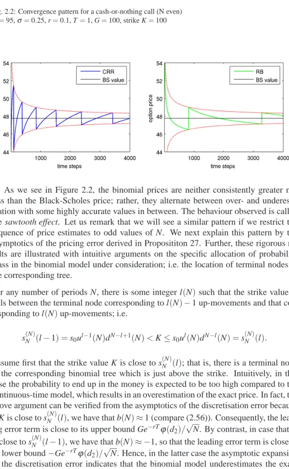
Although the binomial approach is, in principle, an efficient method for lower dimen-sional valuation problems, there are at least two main problems regarding its applica-tion: Firstly, binomial methods often exhibit an irregular convergence behaviour of the option prices computed for an increasing number of periods N. Furthermore, traded op-tions often exhibit discontinuities, so that the Berry-Ess´een inequality on the sequence of binomial price estimates is in general tight; i.e. conventional tree methods converge no faster than in order 1/√N. Unfortunately, the fact that the payoff is non-smooth also causes an irregular convergence behaviour that impedes the possibility to achieve a higher of order of convergence via extrapolation methods. The most prominent ex-ample of irregular behaviour is the so-called sawtooth-effect. Secondly, in multi-asset markets conventional tree construction methods cannot ensure well-defined transition probabilities for arbitrary correlation structures between the assets. As a major aim of the thesis, we present two approaches to ”get binomial trees into shape”; the optimal drift model for the valuation of single-asset options and the decoupling approach to multi-dimensional option pricing.
The optimal drift model is presented as a new binomial scheme for single-asset option pricing. It can lead to convergence of order o(1/N)by exploiting the specific structure of the valuation problem under consideration. The optimal drift model has the poten-tial to outperform even benchmark methods such as the binomial scheme suggested by D.P.J. Leisen and M. Reimer, which is widely used in practice for American op-tion pricing [LR96]. The decoupling approach is presented as a construcop-tion method for multi-dimensional trees. In contrast to the standard approach to multi-dimensional trees, the trees constructed according to the decoupling approach are well-defined for an arbitrary correlation structure of the underlying assets. In addition, they yield a more regular convergence behaviour. In fact, the sawtooth effect can even vanish com-pletely, so that extrapolation can be applied. In contrast to the optimal drift model, the decoupling approach does not assume knowledge of the valuation problem under consideration. We do not claim that the decoupling approach performs best for any particular type of (exotic) option. However, it shows a strong overall convergence be-haviour when applied to arbitrary options. The decoupling approach is therefore an easy and universal approach to cope with the irregular convergence behaviour in multiple dimensions. By contrast, the optimal drift model is based on an advanced construction
technique that shows superior performance if adapted to a specific valuation problem.
An overview of the thesis This thesis consists of two parts; binomial pricing in a single-asset Black-Scholes market and its extension to multi-dimensional situations. In Chapter 2, we give a thorough and rigorous overview of the binomial approach to nu-merical option valuation for a single underlying. We summarise, order and comment on many results from literature. Some of these are well-known, while others are non-standard. In order to complete the picture of the binomial model, we add many pieces of our own work. Furthermore, we introduce the optimal drift model. It is defined by optimising the allocation of probability mass in relation to the strike value, as suggested by Y.S. Tian and by L.-B. Chang and K. Palmer [Tia99], [CP07]. However, while both these models are imposed on the scheme suggested by Cox, Ross and Rubinstein, we optimise the drift of the underlying binomial model. As a result, the optimal drift model can admit convergence of order o(1/N).
In Chapters 3 and 4, we investigate the multi-asset case. Chapter 3 deals with the standard approach to binomial option pricing in a multi-asset Black-Scholes market. Standard methods are based on an approximation of the joint evolution of the underly-ing assets. This will be explained in detail. The standard approach is illustrated with the model suggested by P.P. Boyle, J. Evnine and S. Gibbs which canonically extends the one-dimensional model by Cox, Ross and Rubinstein to a multi-dimensional situa-tion [BEG89]. In addisitua-tion, we consider a multi-dimensional variant of the model sug-gested by Rendleman and Bartter. In order to obtain an appropriate approximation to the multi-asset Black-Scholes model under consideration, the correlation structure among the assets has to be matched. Consequently, the number of moment matching conditions grows quadratically in the dimension. As a result, if we follow the standard approach to multi-dimensional trees, setting up an appropriate binomial model soon gets tedious, and it is sometimes even impossible. On top of that, conventional multi-dimensional tree construction methods inherit the irregular convergence behaviour observed for the one-dimensional situation.
In Chapter 4, the decoupling approach is introduced as an alternative to binomial pricing of multi-asset options. The basic idea of the decoupling approach is to transform the multi-dimensional (log-normal) asset price process to a new process with independent components before setting up a discrete model. The model we suggest contains the 2D example by J. Hull as a special case [Hul06]. Decoupling is an easy approach to over-come the main problems in applications of the standard approach to multi-dimensional trees.
Chapter 4 is essentially based on the paper ”The decoupling approach to binomial pricing of multi-asset options” published in the Journal of Computational Finance [KM09a]. Short extracts from both parts of the thesis are collected in the paper ”Getting multi-dimensional trees into a new shape”, which has recently appeared in the Wilmott Journal [KM09b]. Both papers are joint work with Ralf Korn.
Binomial Pricing for Single-Asset
Options
We consider a one-dimensional Black-Scholes model with stock price dynamics under the risk-neutral measure given by
dS(t) =S(t)(rdt+σdWt), S(0) =s0>0, (2.1)
for some volatility parameter σ >0. Here r is the risk-free interest rate, and W is a one-dimensional Brownian motion with respect to the risk-neutral measure Q. We fix a time horizon T >0.
2.1
Introduction
This chapter deals with binomial pricing of single-asset options. The underlying stock is assumed to follow the Black-Scholes dynamics defined above. From a theoretical perspective, we therefore investigate two-state Markov chain approximations to a geo-metric Brownian motion. To apply the binomial approach to numerical option pricing, we want the approximating models to ensure weak convergence to the stock price pro-cess in the Black-Scholes setting. Under this condition, the corresponding sequence of binomial price estimates converges to the exact option price for most common payoff structures. However, as discussed in the introductory section, conventional binomial schemes suffer from serious problems in practical applications. The convergence be-haviour of the corresponding price estimates is non-monotone and oscillatory. Further-more, if the payoff exhibits discontinuities, the Berry-Ess´een bound on the convergence rate of the pricing error is in general tight. We therefore focus on the construction of binomial approximations that can exploit the structure of the valuation problem under consideration.
Let us briefly outline the contents of this chapter: We first discuss alternative binomial models for the approximation of the stock price process. In particular, we consider
the schemes suggested by Cox, Ross and Rubinstein (1979) (for short: CRR) and by Rendleman and Bartter (1979) (for short: RB). All schemes under consideration are defined so as to asymptotically match the first two moments of the logreturns of the stock price. It is well-known that by asymptotic moment matching, the approximating models converge weakly to the stock price process as the step size in the discrete model tends to zero. This is discussed in detail. Afterwards, we investigate the asymptotic be-haviour of the discretisation error. We demonstrate that for conventional schemes, the Berry-Ess´een bound is tight and the discretisation error converges non-smoothly. This motivates to control the error term, as is done in many advanced models. In particular, we discuss a generalised variant of the advanced models suggested by Tian (1999) and by Chang and Palmer (2007). The latter leads to the new optimal drift model. We will verify that the optimal drift model can admit a superior convergence rate of the dis-cretion error. In Section 2.3, we focus on the application of the binomial approach to numerical option pricing. We see that due to weak convergence, the binomial method can be applied to numerical valuation of most common types of European and Ameri-can options. The corresponding valuation algorithm is called a tree procedure because the possible realisations of the binomial process can be identified with a tree structure. The implementation of binomial option pricing is discussed in detail in Section 2.4. Fi-nally, we analyse the convergence behaviour of binomial trees for the two most common payoff structures; for payoffs that are constant in the terminal value S(T)(i.e. cash-or-nothing options) and for payoffs that are linear in S(T)(i.e. plain vanilla options). We see that amongst the methods under consideration, the shape of the tree constructed by the optimal drift model best exploits the structure of the valuation problem. This results in a superior rate of convergence of the corresponding pricing error.
2.2
Discretisation of the Stock Price and Weak
Conver-gence
In the following, we discuss alternative binomial schemes for the approximation of the stock price process. In the context of numerical option pricing, we want the approxi-mating models to ensure weak convergence to the stock price process S. That is,
Definition 1 (Weak Convergence). Let M be a metric space and let P(N), 1≤N<∞, and P be probability measures on(M,B(M)), where we writeB(M)for the Borelσ
-field of M; i.e. the smallestσ-field containing all open subsets of M. Then we say that the sequence of probability measures(P(N))Nconverges weakly to P, denoted by
if for any bounded, continuous function f : M→R, we have lim N→∞ Z M f(x)P(N)(dx) = Z M f(x)P(dx).
Further, let X(N), 1≤N<∞, and X be random variables with state space M defined on probability spaces(Ω(N),F(N),P(N))and(Ω,F,P), respectively. Then we say that the sequence of random variables(X(N))Nconverges weakly to X, denoted by
X(N)⇒wX,
if for any bounded, continuous function f : M→R, we have, lim
N→∞EP(N)(f(X
(N))) =E
P(f(X))
(compare e.g. [Bil68]).
Remark 1. Of course, weak convergence of random variables is the same as weak
con-vergence of their distributions. In particular, the random variables under consideration need not to be defined on the same probability space, as is used below.
2.2.1
Binomial Models
Let N∈IN denote the number of periods in the discrete model. A binomial approxi-mation to the stock price allows for two possible scenarios per period, so that the path space is naturally given by
E(N):={ω :{1, . . . ,N} → {1,−1}} endowed with the productσ-field
F(N):= N O k=1 P({1,−1}):=σZ(N) k k ∈ N .
HereP(.)denotes the power set and Z(N)
k :E(N) → {1,−1}is the coordinate mapping
Zk(N)(ω) =ωk.
process on(E(N),F(N))by
Sk(N+)1:=Sk(N)eα(N)∆t+β
√
∆t Zk(N+)1
∀k=0, . . . ,N−1, (2.2) for some constantβ >0 and some constantα(N)depending on the number of periods N. Here∆t :=T/N is the grid size of the discrete-time model. In order to achieve weak convergence to the continuous-time price process, we choose the sequence (α(N))N,
the constantβ >0 and the sequence of probability measures(P(N))N on(E(N),F(N))N
such that the following conditions are satisfied:
1. For all N∈IN, the random variables Zk(N), k=1, . . . ,N, (for short: RV) are inde-pendently and identically distributed (for short: i.i.d.).
2. The first two moments of the one-period logreturns of S are asymptotically matched, i.e. we have that
µ(N): = ∆1t EP(N) ln Sk(N+)1 S(kN) S (N) k = α(N) +β q 1 ∆tEP(N) Zk(N+)1 (2.3) σ2(N) := 1 ∆t VarP(N) ln S(kN+)1 S(kN) S (N) k = β2VarP(N) Zk(N+)1 (2.4) are such that as N→∞
µ(N) →r−12σ2 (2.5)
and
σ2(N)
→σ2. (2.6)
Under these conditions, it follows from Donsker’s Invariance Principle (compare e.g. [Bil68], Theorem 10.1) that the linear interpolation of S(N) (suitably scaled in time) converges weakly to the stock price process. Of course, the first condition is satisfied if and only if P(N) is a product measure of the form
P(N)= NN
k=1
for some probability measure P(1,N) on({1,−1},P({1,−1})). Then one-step
transi-tions are independent and they are the same for each period, which we assume from now on. In particular, S(N) is a Markov process.
Introducing the notations pu(N):=P(1,N)({1})and pd(N):=P(1,N)({−1}), the
char-acteristics of the discrete-time modelµ(N)andσ2(N)write as
µ(N) =α(N) +βq1
∆t (2pu(N)−1) (2.8)
and
σ2(N) =4β2p
u(N)(1−pu(N)). (2.9)
Further, pd(N)is determined by pd(N) =1−pu(N). Apparently, we can choose among
an infinite number of possible discretisation schemes that ensure the moment matching conditions (2.5) and (2.6). Let us remark that the drift parameters(α(N))N are allowed
to be non-constant in N. This will provide some additional flexibility to adapt the bino-mial scheme to the payoff structure of interest (compare e.g. [Tia99]); more on that to come later. We impose the following condition:
Assumption 1. The sequence(α(N))N is assumed to be bounded; i.e. it is assumed to
be of order O(1).
In the following, we investigate some widely used binomial schemes. Firstly, we consider transition probabilities that are given by the risk-neutral measure associated with the discrete market consisting of a stock with dynamics (2.2) and a bond
Bk+1=Bker∆t, k=0, . . . ,N−1; B0=1. (2.10)
Here r is the interest rate in the continuous-time model. Let us anticipate that under the risk-neutral measure, the moment matching conditions (2.5) and (2.6) are satisfied if and only if β =σ. By contrast, the drift of the discrete-time model is irrelevant. As explained in the introductory chapter, this approach features an economic insight on option pricing in the Black-Scholes model. When we approximate an option on the continuous-time stock price by evaluating a payoff functional along the sequence of binomial models, the resulting price estimates are themselves option prices in the ap-proximating binomial model.
Secondly, we analyse the discretisation schemes suggested by RB and by CRR1. Here
1The binomial approach suggested by CRR is motivated by its economic insight. However, they
also introduce a binomial model with transition probabilities that are only asymptotically identical with the risk-neutral transition probabilities [CRR79]. In literature, the term CRR model appears both for
the binomial model serves as a plain numerical pricing tool; the binomial estimates for an option on the stock price S do not admit an economic interpretation. In particular, they do not coincide with the corresponding option prices in the binomial model. Hav-ing clarified this conceptual difference to risk-neutral discretisation schemes, we will use the term ”binomial prices” loosely.
Throughout the thesis, we typically distinguish between the discretisation schemes pre-sented above. Below we additionally investigate advanced schemes that allow for a better performance in numerical option valuation.
Discretisation Schemes with Risk-neutral Transition Probabilities In the follow-ing, we consider the discrete-time market consisting of a bond with one-period return er∆t (compare (2.10)) and the stock S(N) with dynamics (2.2). The possible one-period returns of the stock price are denoted by
u(N):=eα(N)∆t+β
√
∆t and d(N):=eα(N)∆t−β√∆t.
By our conventionβ >0, u(N)can be interpreted as the one-period return given that ”the economy is in the good state 1”, and d(N) is the realised one-period return if ”the economy is in the bad state −1”. Then there is the following well-known result (compare e.g. [Bj¨o04], Section 2 and Section 3):
Proposition 1. We have absence of arbitrage opportunities (for short: AAO) in the
discrete market if and only if
d(N)<er∆t<u(N). (2.11)
In this case, the discrete market is also complete and the risk-neutral probability mea-sure is given by Q(N)= NN
k=1
Q(1,N), where
Q(1,N)(1):= ue(r∆tN)−−dd((NN)). (2.12)
Note that (AAO) implies in particular that the measure Q(N) is well-defined. If we write the condition (2.11) in terms ofα(N)andβ, we have (AAO) if and only if
|r−α(N)|pT/N<β.
the discretisation scheme with risk-neutral transition probabilities and for the discretisation scheme with transition probabilities defined by pu(N) =1/2+1/2(r−1/2σ
2
σ p
T/N). In the thesis, we use the term
By Assumption 1, there is some constant M≥0 such that |α(N)| ≤M for all N ∈IN. Thus, we can formulate the following result:
Corollary 1. Provided that the grid size is sufficiently small, the discrete market is
arbitrage-free and complete. It suffices to let N>(r+βM2)2T.
By Corollary 1, we may agree on the assumption that the grid size is always suf-ficiently small to ensure that risk-neutral transition probabilities are well-defined and unique.
As we will see in the following, when we define transition probabilities in accordance with the risk-neutral measure, weak convergence to the continuous-time stock price S is already ensured if we setβ =σ; i.e. it suffices to ensure that the discrete-time stock price is exposed to shocks of appropriate size. Yet this condition is also necessary. By contrast, the drift is irrelevant.
Proposition 2. Assume that the transition probabilities are determined according to
the risk-neutral measure Q(N); i.e. we have Q(N)=NNk=1Q(1,N) with Q(1,N) defined in (2.12). Then the moment matching conditions (2.5) and (2.6) are satisfied if and only if
β =σ.
In particular, convergence to the first two moments of the one-period logreturns in the continuous-time model is of order
µQ(N)(N)−(r−12σ2) =O(N1) and σ2 σ2 Q(N)(N) −1 =O( 1 N), whereµQ(N)(N)andσ2
Q(N)(N)are computed with respect to Q(N)according to (2.3) and
(2.4), respectively.
Proof. By Assumption 1, it follows from a Taylor expansion that u(N) = 1+β T N 1/2 + α(N) +1 2β 2T N+ 1 6β 3+α(N)β T N 3/2 + 1 2α 2(N) +1 2β 2α(N) + 1 24β 4 T N 2 +o 1 N2 (2.13) d(N) = 1−β TN1/2+ α(N) +12β2T N− 1 6β3+α(N)β T N 3/2 + 1 2α2(N) + 1 2β2α(N) + 1 24β4 T N 2 +o 1 N2 , (2.14)
which implies that qu(N):=Q(1,N)(1)is of the form qu(N) = 12+c1(N) TN 1/2 +c3(N) TN 3/2 +o 1 N3/2 , (2.15) where c1(N) = 21β r−α(N)−12β2 c3(N) = 21β 1 2(α(N)−r) 2 +16β2(α(N)−r) + 1 24β4
(compare also [CP07], p. 97/98). Note that c1(N) and c3(N) are of order O(1). We
obtain µQ(N)(N) (2.8) = α(N) +β N T 1/2 (2qu(N)−1) =r−12β2+2βc3(N)NT +o N1 and σ2 Q(N)(N) (2.9) = β24qu(N) (1−qu(N)) =β2−4β2c21(N)TN+o N1 .
Hence, the moment matching conditions (2.5) and (2.6) are satisfied if and only if
β = σ. Moreover, we see from the above equations that the assertion on the order of convergence holds true, which completes the proof.
Remark 2. Let us stress that the moment matching conditions are satisfied
indepen-dently of the particular choice of the sequence(α(N))N.
Further, equation (2.15) implies the following result on the asymptotic behaviour of the risk-neutral measure:
Corollary 2. As the number of periods N tends to infinity,
qu(N) → 12.
The Discretisation Scheme suggested by RB RB suggest to set
α(N) =α :=r−12σ2, β =σ and
Apparently, for this choice the transition probabilities do not depend on the number of periods N. As required, the model satisfies the moment matching conditions (2.5) and (2.6). In fact, moments are not only matched asymptotically, but for any number of periods N; i.e.
µ(N) =r−12σ2 and σ2(N) =σ2.
The Discretisation Scheme suggested by CRR CRR define an appropriate binomial model via α(N) =α :=0, β =σ and pu(N) = 12+12 r−1 2σ 2 σ q T N. (2.17)
In contrast to the RB model, the transition probabilities vary in the number of periods N. In particular, the corresponding probability measures P(N)is only well-defined if the grid size is sufficiently small, which we assume throughout this thesis. To be precise, we need
N ≥ σ12 r− 1 2σ
22T. (2.18)
Simple calculations show that the moment matching conditions (2.5) and (2.6) are satis-fied. In fact, if the model is well-defined for any number of periods N, the first moment of the logreturns is matched exactly. By contrast, the second moment is matched asymp-totically only. We have
σ2(N) =σ2− r−1 2σ2 2 T N, (2.19) which yields σ 2 σ2(N)−1 =O N1 . (2.20)
Note that as the grid size tends to zero, the one-step transition probabilities in the CRR model converge to the corresponding one-step transition probabilities in the RB model. In particular,
pCRRu (N) =pRBu (N) +O√1
N
Further, neither in the CRR model nor in the RB model, the transition probabilities are risk-neutral. However as readily observed from (2.15), there is the following asymptotic relationship between pu(N)and qu(N):
Proposition 3. For the discretisation scheme suggested by RB and by CRR, the one-step
transition probability pu(N), defined in (2.16) and in (2.17), respectively, coincides with
the associated risk-neutral probability qu(N)up to a term of order 1/N3/2. We have that
for the RB model qRBu (N) = 1 2+ 1 24σ 3 T N 3/2 +o 1 N3/2 = pRBu (N) +241 σ3 T N 3/2 +o 1 N3/2
and for the CRR model
qCRRu (N) = 12+21σ r−12σ2NT +41σ (r−16σ2)2+ 1 18σ4 T N 3/2 +o 1 N3/2 = pCRRu (N) + 1 4σ (r− 1 6σ 2)2+ 1 18σ 4 T N 3/2 +o 1 N3/2 .
In particular, Proposition 3 implies the following result:
Corollary 3. Both for the models suggested by CRR and by RB, there is some N0∈IN
such that
qu(N)≥pu(N) for all N≥N0.
In words: For a sufficiently large number of periods N, the chosen probability for an up-movement pu(N)is smaller than the corresponding risk-neutral probability qu(N).
Let us stress that while for the discretisation scheme suggested by RB, the drift enters transition states, it enters transition probabilities for the CRR model. As a conse-quence, the latter implies that the logarithm of the binomial process is symmetric around the starting value. By contrast, the discretisation scheme suggested by RB prefers to have equal weights, which is paid for by a non-symmetric form of the binomial process. Finally, let us anticipate some aspects of the application of the two models to numer-ical option pricing. Firstly, we wish to stress that computing binomial price estimates is cheaper for the RB model because every path has exactly the same probability. For the CRR model, we have to multiply each payment with its specific probability of oc-currence. Secondly, the application of the CRR model suffers from the fact that the requirement (2.18) sets a lower bound on the number of periods N. In particular, if the volatility is small, the transition probabilities are only well-defined for a relative large
number of periods. To illustrate this, let us consider the input parameters r=0.1, T=1 and σ =0.01. Then the number of periods N is bounded from below by 100. For
σ =0.001, the required number of periods is already bounded by 10000.
Time-scaling In the following, we map the binomial process S(N) onto a continuous-time process S(c,N)that appropriately approximates the stock price process S on[0,T]so that weak convergence is ensured. By moment matching, it only remains to scale time appropriately; that is, we apply the transformation k7→k∆t. By linear interpolation, we set S(c,N)(t):=exp N T t +1−NT tln S(N) [N Tt] + NT t−NT tln S(N) [N Tt]+1 , (2.21)
where[x]denotes the greatest integer less or equal to x.
Then for t=k∆t, S(c,N)(t)has the same distribution as Sk(N)and for t ∈ (k∆t,(k+1)∆t), ln(S(c,N)(t))is obtained by linear interpolation between ln(Sk(N))and ln(Sk(N+)1). To moti-vate the time-scaling applied, note that for s=k∆t and t= (k+1)∆t, i.e. t−s=∆t, the log-increment ln(S(c,N)(t)/S(c,N)(s))(asymptotically) matches the first two moments of the log-returns of the stock price process over a period of length∆t.
Weak convergence Due to the Central Limit Theorem, the fact that the pro-cess S(c,N) is based on the binomial distribution becomes negligible in the limit, so that for all times t ∈ [0,T], S(c,N)(t) converges in distribution to the time-t value of time-the stime-tock price St. Moreover, for s = k∆t and t = (k+ 1)∆t,
the log-increment ln(S(c,N)(t)/S(c,N)(s)) = α(N)∆t +βZk(N+)1√∆t is independent of
σ(S(c,N)(u); 0≤u≤s) =σ(Z1(N), . . . ,Z(kN)). Hence, together with the moment matching conditions, we anticipate that the following result holds:
Proposition 4. The sequence of approximating processes(S(c,N))N converges weakly to
the geometric Brownian motion S; for short we write S(c,N) ⇒w S.
Proposition 4 is a key result in the theory of numerical option pricing. It is a simple consequence of Donsker’s Invariance Principle that provides a process version of the Central Limit Theorem. This is discussed in the following. Yet the assertion is not at all non-trivial because all bits of hard work, in particular proving tightness, are hidden in the invariance principle.
Since the RVs Zk(N), k=1, . . . ,N, are i.i.d. for fixed N only, we need a special variant of Donsker’s Theorem that considers triangular schemes:
Theorem 1 (The Invariance Principle for Triangular Schemes). Let ξN1, . . . ,ξNkN be
i.i.d. with mean 0 and variance 0 < σ2
N1 < ∞; put SNi = ∑il=1ξNl, s2Ni = iσN12 ,
and s2N = s2Nk
N. Let X
(N) be the random function that is linear on each interval [s2N,i−1/s2N,s2Ni/s2N] and has values X(N)(s2Ni/s2N) = SNi/sN at the grid points. Then,
X(N)converges weakly to a Brownian motion (compare e.g. [Bil68], problem 1, p. 77).
Remark 3. Note in particular that the above variant of the invariance principle is
applicable to the binomial model suggested by CRR, for which the one-step transition probabilities depend on the number of periods N.
In our application, S(c,N) is a continuous function of the embedded process X(N) defined above. But weak convergence is preserved under continuous mappings. In addition, it is known by Slutsky’s Theorem that an asymptotic matching of moments suffices:
Theorem 2 (Continuous Mapping Principle). Let M and M′ be metric spaces. Let X and X(N), 1≤N<∞, be M-valued RVs and let h : M →M′ be continuous. Then, if X(N)⇒wX , it holds that h◦X(N)⇒wh◦X (compare e.g. [Bil68], Theorem 5.1). Theorem 3 (Slutsky’s Theorem). Let (M,d) be a metric space. Let (X1(N),X2(N))N be
a sequence of(M×M)-valued RVs defined on a probability space(Ω(N),F(N),P(N)).
Suppose that X1(N)⇒wX1for some M-valued RV X1. If for allε >0,
P(N)
d(X1(N),X2(N))>ε→0,
then X2(N)⇒wX1(compare e.g. [EK86], Corollary 3.3.3.).
Proof of Proposition 4. In order to re-write the dynamics of the process Y(c,N)in terms of normalised RVs, we define Yk(N)= r 1 VarP(N) Z(kN) Zk(N)−EP(N)(Z( N) k ) , (2.22)
so that EP(N)(Yk(N)) =0 and VarP(N)(Yk(N)) =1. Then
S(kN+)1 = S(kN)exp α(N)∆t+β√∆t EP(N)(Z(kN+)1) +β r VarP(N) Z(kN+)1√∆t Yk(+N1) = S(kN)expµ(N)∆t+|σ(N)|√∆t Yk(+N1),
which implies that the process S(c,N) writes as S(c,N)(t) =s0eµ(N)t+|σ(N)| √ T Y(c,N)(Tt), t ∈ [0,T], (2.23) with Y(c,N)(s) =√1 N [Ns] ∑ k=1 Yk(N)+ (Ns−[Ns])Y[(NsN)]+1 ! , s ∈ [0,1]. (2.24) Let us define X1(c,N)(t):= r−12σ2t+σ√T Y(c,N) Tt and X2(c,N)(t):=ln St(c,N) =µ(N)t+|σ(N)|√T Y(c,N) Tt. Then X (c,N) 1 −X (c,N) 2 ∞= sup t∈[0,T] (r−12σ 2−µ(N))t+ (σ− |σ(N)|)√T Y(c,N) t T
measures ”the impact of an asymptotic matching of moments” in terms of the sup-norm, i.e.||f||∞=supt∈[0,T]|f(t)|. Letε>0. Apparently,
P(N)X1(c,N)−X2(c,N) ∞>ε ≤ P(N) µ(N)−(r−12σ2)T > ε2+ P(N)(σ− |σ(N)|)√T Y(c,N) Tt ∞> ε 2 . (2.25)
For a sufficiently large number of periods N, the first term on the right-hand side of equation (2.25) is zero by asymptotic moment matching. It remains to investigate the second term. Clearly,
P(N) (σ− |σ(N)|) √ T Y(c,N) Tt ∞> ε 2 = P(N) |σ− |σ(N)||√T max k=1,...,N M (N) k > ε2 ,
where the discrete process M(N)is defined by Mk(N):= √1 N N ∑ i=1 Yi(N), 1≤k≤N, M0(N):=0. (2.26)
As M(N)is a discrete martingale, it follows from Doob’s martingale inequality (compare e.g. [Dur05], Theorem 4.4.2) that
P(N) |σ− |σ(N)||√T max k=1,...,N M (N) k > ε2 ≤ 4 ε2(σ− |σ(N)|) 2 T EP(N) M (N) N 2 = ε42(σ− |σ(N)|) 2 T. (2.27)
By the moment matching conditions, the right-hand side of inequality (2.27) tends to zero as N tends to infinity, which implies that
P(N) X (c,N) 1 −X (c,N) 2 ∞>ε →0.
Consequently, according to Slutsky’s Theorem it suffices to consider the process X1(c,N) instead of X2(c,N).
Further, the invariance principle for triangular schemes applies to the sequence (Y(c,N))N; i.e.
{Y(c,N)(s)}{s∈[0,1]}⇒w{B(s)}{s∈[0,1]}, (2.28)
where {Bs,F˜s; 0 ≤ s ≤ 1} is a Brownian motion. Define the time-change
t : [0,1] →[0,T]by
t : s →T s and the filtration Ft := F˜
t/T indexed according to the ”new time”. Then by
the time-scaling property of Brownian paths (compare [KS98], Lemma 2.9.4), {Wt,Ft; 0≤ t ≤ T}with
Wt :=√T B(t/T) 0≤ t ≤ T
is again a Brownian motion. Consequently, according to the continuous mapping prin-ciple, (2.28) implies that
s0exp
X1(c,N)
⇒wS,
which proves the assertion.
2.2.2
Distributional Fit
In the following, we investigate how well the process S(c,N) fits the stock price process S for a fixed time t ∈[0,T]; i.e. we are interested in the distance
d(N)(t,x):= P(N) S(tc,N)≤x −Q(St≤x) .
The Minimal Convergence Rate
The Berry-Ess´een inequality suggests that the distance d(N)(t,x)converges to zero in order 1/√N uniformly in x∈R. Yet in our application, the moments are only asymp-totically matched. We see in the following that if the moments themselves converge in order 1/√N, the Berry-Ess´een bound is maintained.
Theorem 4 (Berry-Ess´een inequality). Let X1, . . . ,XN be independent RVs such that
EXj=0, E|Xj|3<∞(j=1, . . . ,N). We write σ2 j =EX2j, BN = N ∑ j=1σ 2 j, F(N)(x) =P B− 1/2 N N ∑ j=1 Xj<x ! and L(N)=B−N3/2 ∑N j=1 E|Xj|3. Then, sup x F(N)(x)−Φ(x) ≤A L(N),
where Φ(x)denotes the standard normal distribution function and A is some positive constant (compare e.g. [Pet75], Theorem 5.3).
Proposition 5. Suppose that S(N)is the binomial process (2.2) with |µ(N)−µ| = O 1 √ N and ν 2 σ2(N)−1 = O 1 √ N (2.29)
for some constantsµ,ν ∈R,ν >0. Then for all times t ∈ [0,T], sup x P(N) S(c,N)(t)<x −Φ ln x s0 −µt ν√t ! = O 1 √ N . (2.30)
Remark 4. Forµ =r−1/2σ2andν =σ, the condition (2.29) is a sharpening of the moment matching conditions (2.5) and (2.6). It additionally requires a minimal order of convergence.
Proof of Proposition 5. Note that
Φ ln x s0 −µ(N)t |σ(N)|√t ! =Φ ln x s0 −µt ν√t ε (N) 1 +ε (N) 2 ! , (2.31)
whereεi(N)(i=1,2)are the correction terms
ε(N) 1 = |σ(νN)| and ε (N) 2 = (µ−µ(N))t |σ(N)|√t
that appear because the constants µ and ν are only asymptotically matched. By the triangular inequality, sup x P(N) S(c,N)(t)<x −Φ ln x s0 −µt ν√t ! ≤ sup x P(N) S(c,N)(t)<x −Φ ln x s0 −µ(N)t |σ(N)|√t ! + sup x Φ ln x s0 −µ(N)t |σ(N)|√t ! −Φ ln x s0 −µt ν√t ! .
Using definition of the correction termsε1(N) andε2(N), we further observe that
sup x Φ lnx s0 −µ(N)t |σ(N)|√t ! −Φ ln x s0 −µt ν√t ! = sup x Φ ln x s0 −µt ν√t ε (N) 1 +ε (N) 2 ! −Φ ln x s0 −µt ν√t ! ≤ sup x Φ x+ε2(N)−Φ(x) +sup x Φ xε1(N)−Φ(x)
Thus, in total, sup x P(N) S(c,N)(t)<x −Φ ln x s0 −µt ν√t ! ≤ sup x P(N) S(c,N)(t)<x −Φ ln x s0 −µ(N)t |σ(N)|√t ! + sup x Φ x+ε2(N)−Φ(x) +sup x Φ xε1(N)−Φ(x) (2.32)
In the following, we investigate each term on the right-hand side of the inequality above. The first term can be written as
sup x P(N) S(c,N)(t)<x −Φ ln x s0 −µ(N)t |σ(N)|√t ! = sup x P(N) S(c,N)(t)<s0eµ(N)t+|σ(N)| √ tx −Φ(x) = sup x P(N) √1 t N/T [t N/T] ∑ j=1 Yj(N)+ tNT −tNTY[(t NN)/T]+1 ! <x ! −Φ(x) ,
where Yk(N)are the normalised RVs defined in (2.22). Hence, we observe that
sup x P(N)S(c,N)(t)<x−Φ ln x s0 −µ(N)t |σ(N)|√t ! ≤ max ( sup x P(N) √1 t N/T [t N/T] ∑ j=1 Yj(N)+qtNT −tNT Y[(t NN)/T]+1 ! <x ! −Φ(x) , sup x P(N) q 1 [tNT]+1 [t N/T] ∑ j=1 Yj(N)− Y (N) [t N/T]+1 ! <x ! −Φ(x) )
Note from applying the Berry-Ess´een inequality to both arguments on the right-hand side of the inequality above that
sup x P(N)S(c,N)(t)<x−Φ ln x s0 −µ(N)t |σ(N)|√t ! = O√1 N . (2.33)
It remains to consider the last two terms on the right-hand side of inequality (2.32) that are due to the presence of the correction termsε1(N)andε2(N). By assumption (2.29), we have ε(N) 1 2 =1+h(N),
where for sufficiently large N,
|h(N)| ≤ Nc
for some constant c>0. Consequently, we obtain by the Binomial Series Theorem that ε (N) 1 −1 = O 1 √ N . (2.34) Further, ε (N) 2 = (µ−µ(N))t ν√T ε (N) 1 ≤ (µ−µ(N))t ν√T ε (N) 1 −1 + (µ−µ(N))t ν√T = O 1 √ N . (2.35)
By the Mean-Value Theorem, there is someΘ(xN,1)∈[0,1]such that sup x Φ xε1(N) −Φ(x) ≤ sup x Φ′ x+Θ(xN,1)ε1(N)−1 x x ε (N) 1 −1 ≤ sup x |Φ ′(x)x|sup x x x+Θ(xN,1)ε1(N)−1x ε (N) 1 −1 .
AsΦ′(x)x is bounded, it follows from (2.34) that sup x Φ xε1(N) −Φ(x)=O 1 √ N . (2.36)
Similarly, there isΘ(xN,2)∈[0,1]such that sup x Φ x+ε2(N)−Φ(x) ≤ sup x Φ′ x+Θ(xN,2)ε2(N)ε2(N).
Hence, by boundedness ofΦ′(x), (2.35) implies that sup x Φ x+ε2(N)−Φ(x) =O 1 √ N . (2.37)
Finally, the assertion follows by combining the results (2.33), (2.37) and (2.36).
Letµ =r−1/2σ2andν =σ. As discussed previously, for the RB model the mo-ment matching conditions (2.5) and (2.6) are satisfied exactly, i.e. they hold for any number of periods N. By contrast, for the CRR model the volatility is asymptotically matched only. Here σ2/σ2(N) converges to one in order 1/N. Further according to
Proposition 2, if we use risk-neutral transition probabilities, the corresponding charac-teristicsµ(N)andσ2(N)of the discrete-time model converge in order 1/N if and only if β =σ. Hence by Proposition 5, for the models under consideration, convergence to the limiting moments is sufficiently fast to maintain the minimal convergence rate 1/√N suggested by the Berry-Ess´een inequality:
Corollary 4. Let S(N)be the process suggested by CRR, the process suggested by RB or any binomial process (2.2) withβ =σ and risk-neutral transition probabilities. Then for any time t ∈ [0,T],
sup x P(N) S(c,N)(t)<x −Q(S(t)<x) =O 1 √ N (2.38)
Remark 5. The Berry-Ess´een inequality sets a lower bound on the convergence rate
of the discretisation error in the approximation to the stock price. It depends on the specific distribution of the discrete-time model whether this minimal convergence rate is attained. Of course, the convergence rate of the discretisation error can also be faster.
For the RB model, it is easy to observe that the Berry-Ess´een inequality is tight:
Proposition 6. Let S(NN)be the terminal value of the RB model. Then the distributional fit at the median of the continuous-time model x =s0e(r−1/2σ
2)T is of the following order: P(N) S(NN)<s0e(r−1/2σ 2)T −12 =0 for N odd, and lim N→∞ N even P(N) S(NN)<s0e(r−1/2σ 2)T −1 2 1 √ 2π √ N = 1.
Proof. The RB model is tilted in such a way that P(N)SN(N)<s0e(r−1/2σ
2)T
where X is a Bin(N,1/2)-RV on some probability space(Ω,A,P). Further, it follows
from symmetry that
P X < N2 = 12 1−P X =N2 = 1 2 1− NN/221N N even 1 2 N odd
Finally, by Stirling’s formula (compare e.g. [AS72], Formula 6.1.38), we have
N N/2 1 2N = 2 √ 2π 1 √ N+o 1 √ N ,
which yields the assertion.
We see that the RB model leads to a terminal value S(NN), for which the Berry-Ess´een bound is tight in the sense that
lim sup N→∞ ( sup x P(N)S(NN)<x−Φ ln x s0 −(r−1 2σ 2)T σ√T ! √ N ) ≥ lim sup N→∞ n P(N) S(NN)<s0e(r−1/2σ 2)T −12 √ N o = √1 2π >0.
In the general case, it is more involved to decide whether the Berry-Ess´een inequality is tight. In the next paragraph, we investigate the asymptoptic behaviour of the dis-cretisation error for a fairly general class of binomial processes. We will essentially follow Chang and Palmer (2007). However, while they restrict to risk-neutral transition probabilities, we take a more general approach, so that our results also apply to the models suggested by CRR and by RB. In particular, we will find that the Berry-Ess´een inequality is tight for the models under consideration.
The Asymptotic Behaviour of the Discretisation Error
For simplicity, we limit the following analysis of the discretisation error to the terminal distribution of the stock price. For the Black-Scholes model, the distribution at maturity is given by
where
d2:=d2(x):=ln(s0/x)+(r−1/2σ 2)T
σ√T .
Let us assume that the drift in the discrete-time model is constant in N; i.e.α(N)≡α. As we see in the following, even in this case there is no asymptotic expansion of P(N)
S(NN)≥x
around Q(ST ≥x) =Φ(d2)in the conventional sense. That is, a
func-tion f(ε)has an asymptotic expansion in powers ofε up to order k with constant coef-ficients(ci)i=0,...,k, if for any m=0, . . . ,k,
lim ε→0+ε −m f(ε)− ∑m i=0 ciεi =0.
However, as suggested by Diener and Diener [DD04], the asymptotic behaviour of the discretisation error can be described with an appropriate ”extended asymptotic calcu-lus”. Let us explain: Apparently, the distribution of the binomial process at maturity P(N) S(NN)≥x writes as P(N)S(NN)≥x= ∑N i=l(N) N i pu(N)i(1−pu(N))N−i=: Fx(N),
where l(N) is the smallest integer l such that s0u(N)ld(N)N−l ≥x. If α(N) is
con-stant in N, it follows from a Taylor expansion that u(N)and d(N)admit an asymptotic expansion in powers of 1/√N up to an arbitrary order k in the conventional sense. Consequently, we might be tempted to suppose that if pu(N)admits an asymptotic
ex-pansion in powers of 1/√N in the conventional sense (which is in particular valid for the models under consideration), the distribution Fx(N)will do so, too. However, there
are pr