Path Planning Algorithms for Autonomous Mobile Robots
MohammadAli AskariHemmat
A Thesis in The Department ofMechanical, Industrial and Aerospace Engineering
Presented in Partial Fulfillment of the Requirements for the Degree of Master of Applied Science at
Concordia University Montr´eal, Qu´ebec, Canada
July 2018
c
CONCORDIA UNIVERSITY School of Graduate Studies
This is to certify that the thesis prepared
By: MohammadAli AskariHemmat
Entitled: Path Planning Algorithms for Autonomous Mobile Robots
and submitted in partial fulfillment of the requirements for the degree of
Master of Applied Science (Mechanical Engineering)
complies with the regulations of this University and meets the accepted standards with respect to originality and quality.
Signed by the final examining committee:
Dr. Suong Van Hoa Chair
Chair’s name
Dr. Javad Dargahi Examiner
Examiner’s name
Dr. Wei-Ping Zhu Examiner
Examiner’s name
Co-Supervisor Co-Supervisor’s name
Dr. Youmin Zhang Supervisor
Supervisor’s name Approved by
Chair of the MIAE Department 2018
ABSTRACT
Path Planning Algorithms for Autonomous Mobile Robots MohammadAli AskariHemmat
This thesis work proposes the development and implementation of multiple differ-ent path planning algorithms for autonomous mobile robots, with a focus on differdiffer-entially driven robots. Then, it continues to propose a real-time path planner that is capable of find-ing the optimal, collision-free path for a nonholonomicUnmanned Ground Vehicle(UGV) in an unstructured environment. First, a hybrid A* path planner is designed and imple-mented to find the optimal path; connecting the current position of the UGV to the target in real-time while avoiding any obstacles in the vicinity of the UGV. The advantages of this path planner are that, using the potential field techniques and by excluding the nodes surrounding every obstacles, it significantly reduces the search space of the traditional A* approach; it is also capable of distinguishing different types of obstacles by giving them distinct priorities based on their natures and safety concerns. Such an approach is essential to guarantee a safe navigation in the environment where humans are in close contact with autonomous vehicles. Then, with consideration of the kinematic constraints of the UGV, a smooth and drivable geometric path is generated. Throughout the whole thesis, exten-sive practical experiments are conducted to verify the effectiveness of the proposed path planning methodologies.
ACKNOWLEDGEMENTS
I would like to express my deepest gratitude to my supervisor, Dr. Youmin Zhang, for his excellent guidance, caring, patience, and providing me with an excellent atmosphere for doing research. This thesis would not have been possible without his guidance and support. I would like to thank all my fellow researchers and colleagues in Networked Autonomous Vehicles (NAV) Lab at Concordia University. Without their guidance, support and continual encouragements, this thesis would not have been possible. I am especially grateful to Dr. Zhixiang Liu , Ban and Dr. Yiqun Dong. They have proven to be supportive friends as well as thoughtful colleagues with good advice and collaboration. Finally, my deepest and most heartfelt thanks to my family; my parents who provided the best possible environment for me to grow up and supported me in all my pursuit and my brother and sister for all their love and encouragement.
TABLE OF CONTENTS
LIST OF FIGURES . . . ix
LIST OF ACRONYMS . . . xii
1 Introduction 1 1.1 Motivation and context . . . 2
1.2 Problem description . . . 3
1.3 Structure of the thesis . . . 4
2 Mathematical Modeling 5 2.1 Introduction . . . 5
2.2 Kinematic model for differentially driven robots . . . 5
2.3 Controlling a differentially driven robot . . . 7
2.3.1 Accessibility and controllability . . . 10
2.3.2 Configuration space . . . 10
2.3.3 Configuration space obstacles . . . 11
2.3.4 Definition of a motion planning problem . . . 12
3 Potential Functions 16 3.1 Introduction . . . 16
3.2 Potential field forC =R2 . . . . 19
3.3 Attractive potential . . . 20
3.4 Repulsive potential . . . 22
3.5 Motion planning using APF . . . 23
3.5.1 Continuous motion planning . . . 24
3.5.2 Navigation functions . . . 34
3.5.2.1 Navigation functions in a sphere world . . . 36
3.5.2.2 Navigation functions in a star world . . . 44
4 Heuristic-Based Path Planning 51
4.1 Graph basics . . . 51
4.2 Breadth first search . . . 56
4.3 Depth first search . . . 58
4.4 Dijkstra search . . . 60 4.5 A* search . . . 61 4.5.1 Heuristics . . . 64 4.5.2 Admissibility . . . 67 4.6 Hybrid A* . . . 67 4.6.1 Dubin’s path . . . 68 4.6.2 Action space . . . 69 4.6.3 Node expansion . . . 71 4.6.4 Analytical expansion . . . 73 4.6.5 Heuristics . . . 73 4.6.6 Constrained heuristics . . . 74 4.6.7 Unconstrained heuristics . . . 75
5 Implementation & Results 78 5.1 General structure of experiments . . . 79
5.1.1 Software . . . 79
5.1.2 Hardware . . . 79
5.1.3 Mobile robot . . . 79
5.2 Path planner structure . . . 80
5.2.1 Localization . . . 82
5.2.2 Occupancy grid . . . 82
5.2.3 Search . . . 82
5.3 Path smoothing . . . 85
5.4 Path tracking . . . 91
6 Conclusions & Future Works 100
6.1 Conclusions . . . 100
6.2 Future works . . . 101
6.2.1 Dynamic path planning . . . 101
6.2.2 Localization . . . 101
6.2.3 Acceleration and velocity profiles . . . 102
LIST OF FIGURES
1.1 Google trends result for theAutonomous CarsandDarpa Grand Challenge
queries . . . 2
2.1 Geometry of a generic differentially driven robot [22] . . . 7
2.2 A visualization ofConfiguration Spacefor a double pendulum [5] . . . 11
2.3 AWork Spacewith start and goal states of a 2D rigid body [5] . . . 14
2.4 A configuration space with start and goal states of a rigid body [5] . . . 15
3.1 The total potential field is simply the sum of the attractive and repulsive fields 18 3.2 Negated gradient vector field . . . 19
3.3 Conic potential field . . . 21
3.4 Smooth & differentiable attractive potential field . . . 22
3.5 Equipotential contour of repulsive function around obstacles . . . 23
3.6 A work space with rectangular obstacles . . . 26
3.7 Planned path generated by simple integration with oscillations . . . 27
3.8 Planned path by updatingα at each iteration . . . 29
3.9 Dynamics ofα as a function of number of iterations . . . 30
3.10 General gradient descent on different start/goal configurations might not converge . . . 31
3.11 Planned path by updatingα at each iteration . . . 32
3.12 Local minima in a workspace when the direction of movement is perpen-dicular to one of the obstacles in the workspace . . . 33
3.13 There is no deterministic gradient descent algorithm to solve the local min-ima problem . . . 34 3.14 Lavalle et. al. [25] proposed an algorithm to use cell decomposition and
3.15 Choset et. al. [6] used the weak harmonic potential functions on
decom-posed cells . . . 35
3.16 Different sets on a sphere world with respective dimensions . . . 38
3.17 ASphere Worldworkspace . . . 41
3.18 Change in the contour lines over free space asKincreases . . . 42
3.19 Change in the scalar field over free space asKincreases . . . 43
3.20 (a) Shows a simple work space with 2 rectangular obstacles and (b) Shows the occupancy grid representation of the same work space. Cells that lie on an obstacle have a value of 1 and the free cells have a value of zero . . . 46
3.21 Comparing a 4-neighborhood and an 8-neighborhood connectivity . . . 47
3.22 Wave front planner growing inside a workspace . . . 48
3.23 Wave front planner growing inside a workspace different colors represent different cost of a cell . . . 49
3.24 A path found using gradient descent is shown on the grid, and the same path is shown on the work space . . . 50
4.1 A graph with 7 nodes and 8 edges. The label represents the cost of moving from nodeVitoVj. . . 52
4.2 A grid represented as a graph . . . 53
4.3 BFS state space . . . 58
4.4 DFS state space . . . 60
4.5 Dijkstra state space . . . 61
4.6 A* state space . . . 62
4.7 A* Search using manhattan heuristic . . . 66
4.8 A* Search using euclidean heuristic . . . 66
4.9 Dubin’s path . . . 68
4.10 Generic discrete A* vs hybrid continuous A* [12] . . . 72
4.11 Euclidean heuristic, visited nodes: 3011 Path Length: 7.567432 m . . . 74 4.12 Constrained Dubins heuristic, visited nodes: 2213 Path Length: 7.408262 m 75
4.13 Unconstrained Heuristic, Visited Nodes: 107 Path Length: 7.617800 m . . . 76
5.1 Quanser Ground Vehicle, QGV . . . 80
5.2 Hybrid A* path planner . . . 81
5.3 Flex 3 OptiTrack motion capture system . . . 82
5.4 Work Space . . . 83
5.5 Cost map of a work space . . . 84
5.6 Hybrid A* path . . . 85
5.7 Smooth Hybrid A* path . . . 89
5.8 Hybrid A* path vs a smooth hybrid A* path . . . 90
5.9 Empirical comparison of tracking results [25] . . . 92
5.10 Geometry of Pure-Pursuit algorithm . . . 93
5.11 Hybrid A* search in a dynamic environment . . . 94
5.12 Dynamic Hybrid A* - configuration 1 . . . 95
5.13 A depiction of cross-track errors along X & Y axes in(m)at configuration 1 95 5.14 Dynamic Hybrid A* - configuration 2 . . . 96
5.15 A depiction of cross-track errors along X & Y axes in(m)at configuration 2 96 5.16 Dynamic Hybrid A* - configuration 3 . . . 97
5.17 A depiction of cross-track errors along X & Y axes in(m)at configuration 3 97 5.18 Dynamic Hybrid A* - configuration 4 . . . 98
5.19 A depiction of cross-track errors along X & Y axes in(m)at configuration 4 98 5.20 Dynamic Hybrid A* - configuration 5 . . . 99 5.21 A depiction of cross-track errors along X & Y axes in(m)at configuration 5 99
LIST OF ACRONYMS
LTI Linear Time Invariant
PID Proportional —Integral —Derivative
MP Motion Planning
PP Path Planning
RTOS Real Time Operating System
ML Machine Learning
GD Gradient Descent
AGD Adaptive Gradient Descent
AI Artificial Intelligence
RT Real Time
PF Potential Function
APF Artificial Potential Function
LIFO Last In First Out
FIFO First In First Out
BFS Breadth First Search
DFS Depth First Search
Chapter 1
Introduction
The topic of path planning for mobile, car-like, robots has consistently been in the center of attention for the past thirty years. Researches are still proposing new algorithms with higher performance and accuracy. During the last decade, improvements in computational power, easier and cheaper access to hardware and software platforms has helped researches develop innovative algorithms and build on top existing ones. Algorithms that implementing them might have been unfeasible a few years ago, are now being implemented on robots thanks to cheap, fast and affordable hardware.
There are different challenges inPath Planningfor mobile robots. However, the final goal of all algorithms is to find an optimal and safe path. Optimality of a path can be interpreted differently based on the use case but usually optimality of a path implies how short the path is. A safe path on the other hand is a path that guides the robot to safely travel around obstacles, both static and dynamic ones.
Based on the application, there might be solutions to the path planning problem but they are usually designed with limiting assumptions in mind, assumptions that render the algorithm and solution useless in another scenario or under slightly different assumptions. There have been numerous attempts in the past 20 years to improve the cruise control of cars and not only help the drivers with monitoring and controlling the speed but also with lane changing and navigation. The current solutions usually depend on visual lane finding techniques and driving the car within a lane. However, as soon as the markings on the road
to perform research on the provided platform.
In this thesis, the focus is to analyze different path planning algorithms which were developed over years and evaluate their strengths and weaknesses. The feedback control approaches to solve the path planning problem has usually failed. The main reason is that feedback control has traditionally approached this problem where the work space and environment is free of obstacles, or the obstacles are static. The attempts to provide a feedback control law in presence of obstacles are usually extremely limited in practice. This work will present such attempts and will discuss why they are so limited and then propose a set of feasible solutions that are relatively easy to implement as base path planner and then expand upon with a more sophisticated algorithm. The proposed algorithms do not depend on strong mathematical background and are fast enough to find collision free paths even in dynamic workspaces.
1.2
Problem description
The goal of this thesis is to provide enough resources to solve a rather generic path planning problem. The path planning problem can be summarized as:
Generating a smooth path in real-time that is drivable by a nonholonomic robot. The smooth, optimal path should start from an arbitrary state xsand should end in an arbitrary set XGoal while avoiding static and dynamic obstacles. The algorithm should explicitly de-termine if there is no valid path between initial and goal configurations.
Historically this has been the definition of a path planning problem [25]. The path planners usually assume perfect sensing for localization and exact control. This implies that the workspace and the robot’s state is perfectly known at all times. In this thesis a set of similar assumptions are made:
• The localization is a solved problem and we have the exact location and state of the robot and obstacles with high certainty and low latency at all times.
• The size of the obstacles are large enough to be detected by the localization system.
• Dynamic obstacles will only move in a short time span and will stay rested for the majority of the time.
1.3
Structure of the thesis
In Chapter 2, a short background for nonholonomic systems is given and theoretical con-cepts for controlling such systems are presented. Chapter 3 and Chapter 4 go through different approaches to solve the path planning problem and will discuss how these algo-rithms have failed to provide a solution for the problem. Chapter 5 will use the theoretical foundation presented in Chapter 4 and proposes a solution. The implementation details and results are also discussed in this chapter. Finally, in Chapter 6 some suggestions for future work is presented and the shortcomings of the proposed algorithm is discussed.
Chapter 2
Mathematical Modeling
2.1
Introduction
In order to design controllers for systems, one should first know how the system functions and behave. The differential drive robot is one of the most common models used in robotics research due to multiple reasons which will become apparent in this chapter. In Section 2.2 the kinematic model of a differential wheeled robot is derived. Then it is shown that it is a driftless control-affine system and then its controllability is discussed [22].
2.2
Kinematic model for differentially driven robots
Differential drive robots are very popular for indoor robotic experiments because they are very easy to build from scratch due to their simple structural design. The kinematic model is also very intuitive and easy to derive and maybe the most appealing reason is the simple control laws required to control such systems. The robot has 2 main wheels, each of which is powered independently using a DC motor. To add stability to the robot and preventing it from falling a third passive wheel, caster wheel, is added to the rear/front of the robot. The steering of the robot is maintained by rotating the wheels at different rates and thus move the robot around the environment.
motions, pure translation and pure rotation. Assuming non-zero angular velocity, if the velocities have the same magnitude and the same sign ur =ul, the robot wheel have a pure translational motion and if the signs are oppositeur=−ul, the robot will have a pure rotational motion.
By controlling the angular velocity of the two wheels one could control the motion of the robot in the working space. So the control vector becomes the angular velocity of the right and left wheels.
u= (ul, ur) (2.1)
We are interested to know where the robot is located in a fixed reference frame and at which direction it is heading to so the state vector, configuration vector, of the system is
[x, y, θ]T. Since there are only two control inputs and the system has 3 states, we have an under-actuated system. Now, the question is which point on the robot should we care about and control, a point at the front, a point on the wheel, or some where else?
In a pure rotational motion ur =−ul, the middle point of the axle between the two wheels does not move. Assigning the origin of the local coordinate system on the middle point would satisfy the pure rotational motion because that point does not have any translational motions under this condition. So it would be easier to analyze the system by selecting such coordinate system. If the position of this point and the orientation of the local frame with respect to the global reference frame is known at all times one could localize the entire system.
As it can be observed from Figure 2.1 there are only 2 geometrical measurements necessary to construct the kinematic model of a differential drive robot. The vertical dis-tance between the center of the two wheels L and the radius of the wheels r. Assuming two arbitrary velocities for the right and left wheels and by using instantaneous center of velocity the the linear and angular velocity of the mid-point can be easily found.
˙
θ = vR−vL
Figure 2.1: Geometry of a generic differentially driven robot [22]
v=vR+vL
2 (2.3)
and by assuming the radius of each wheel isrthe linear velocity isvR=r×uRand substi-tuting it in equation 3 would yield:
˙
θ = r
L(ur−ul) (2.4)
Now that the angular and linear velocity of the mid-point is known, it is easy to derive the state-transition equation. In order to find the projection of the velocity on the xandyaxis simply multiply the linear velocityv, by cosθ and sinθ.
˙ x=vcosθ ˙ y=vsinθ ˙ θ =ω (2.5)
2.3
Controlling a differentially driven robot
Rewriting the kinematic model of the differential drive robot, Equation (2.5), in matrix form would yield
˙ x ˙ y ˙ θ = cosθ 0 sinθ 0 0 1 v ω (2.6)
and in vector form it will be
˙
q=Au (2.7)
comparing Equation (2.7) to differential equation model of a linear system
˙
q= f(q,u) =Aq+Bu (2.8)
we notice that it is not a linear system so it must be nonlinear. The general form of a first-order nonlinear equation is
˙
q=f(q, u, t) (2.9) and if the system is affine in control input the general form will be
˙
q=f1(q, t) +f2(q, t)u (2.10) Equation (2.10) represents a family of nonlinear differential equations called control affine systems. These systems are linear in action but the states of the system evolve in a nonlinear fashion [22]. If the first term f1(q,t), is zero, the system becomes a driftless nonlinear
control system.
˙
q=f2(q, t)u (2.11) By comparing Equation (2.11) and Equation (2.7) it is trivial that the kinematic model of the differential drive robot is indeed a driftless nonlinear system. The nonholonomic nature of wheeled mobile robots has precise consequences in terms of structural properties of the kinematic model. The first, and most important one, is that in spite of the reduced number of degrees of freedom, wheeled robot is controllable in its configuration space; i.e.,
given two arbitrary configurations, there always exists a kinematically admissible trajectory (with the associated velocity inputs) that transfers the robot from one to the other. Since the kinematic model is driftless, a well known result implies that it is controllable if and only if the accessibility rank condition holds. The motion control problem for wheeled mobile robots is generally formulated with reference to the kinematic model.
There are essentially two reasons for taking this simplifying assumption. First, the kinematic model fully captures the essential nonlinearity of single-body wheeled robots, which stems from their nonholonomic nature. This is another fundamental difference with respect to the case of robotic manipulators, in which the main source of nonlinearity is the inertial coupling among multiple bodies. Second, in mobile robots it is typically not possible to directly command the wheel torques, because there are low-level wheel control loops integrated in the hardware or software architecture. Any such loop accepts as input a reference value for the wheel angular speed, which is then reproduced as accurately as possible by standard regulation actions (e.g., PID controllers). In this situation, the actual inputs available for high-level control are precisely these reference velocities.
Several methods are available to drive a wheeled mobile robot in feedback along a desired trajectory. A straightforward possibility is to first compute the linear approximation of the system along the desired trajectory (which, unlike the approximation at a configu-ration, results to be controllable) and then stabilize it using linear feedback. Only local convergence, however, can be guaranteed with this approach. For the kinematic model of the unicycle, global asymptotic stability may be achieved by suitably morphing the linear control law into a nonlinear one [10].
In robotics, a popular approach for trajectory tracking is input - output linearizion via static feedback. In the case of a unicycle, consider as output the Cartesian coordinates of a pointBlocated ahead of the wheel, at a distancebfrom the contact point with the ground. The linear mapping between the time derivatives of these coordinates and the velocity con-trol inputs turns out to be invertible provided thatbis nonzero; under this assumption, it is therefore possible to perform an input transformation via feedback that converts the unicy-cle to a parallel of two simple integrators, which can be globally stabilized with a simple
proportional controller (plus feedforward). This simple approach works reasonably well. However, if one tries to improve tracking accuracy by reducing b (so as to bring B close to the ground contact point), the control effort quickly increases. Trajectory tracking with b
(i.e., for the actual contact point on the ground) can be achieved using dynamic feedback linearizion. In particular, this method provides a one-dimensional dynamic compensator that transforms the unicycle into a parallel of two double integrators, which is then glob-ally stabilized with a proportional-derivative controller (plus feedforward). In contrast to static feedback linearizion, no residual zero dynamics is present in the transformed system. However, the dynamic compensator has a singularity when the unicycle driving velocity is zero. This is expected, because otherwise the tracking controller would represent a univer-sal controller. Note that dynamic feedback realizability using thex, youtputs is related to them being flat, the two properties are equivalent.
2.3.1
Accessibility and controllability
For linear systems,x=Ax+Buwherex∈Rnandu∈Rmand the celebrated Kalman rank condition fully characterizes when the system is (globally) controllable (from any point). Our objective here is to come up with similar tests for nonlinear systems. Let us start by making precise the notions of accessibility and controllability [10].
2.3.2
Configuration space
It is easy to imagine the height of the robot does not have any effect on the motion planning algorithm and the generated paths so let’s consider the 3-D rigid body of the robot does not have a height, the result would be a 2-D plane. So the motion planning algorithm must generate a path for the new rigid body, the plane, inR2. As mentioned in Section 2.3 the
transformation matrix Equation (2.6) on page 8 could transform any x,y∈R this would
yield a manifold M1 =R2. Also one could apply any rotation θ ∈[0,2π) which would
C={(x,y,θ)|(x,y)∈R2,θ ∈[0,2π)]}=R2×S1=M1×M2 (2.12)
The new manifold is called the Configuration Space of the system and might be considered as a special case of the state space [22]. The configuration space of the system looks like a torus but the cross section is a square instead of a circle. Topologically speaking, it is important to realize the configuration space is not bounded and it does not have a boundary.
Figure 2.2: A visualization ofConfiguration Spacefor a double pendulum [5]
Figure 2.2 shows how the systems moves in the configuration space. As it can be seen due to the periodic nature of rotations the system reaches it’s starting yaw angle after a complete rotation.
It is crucial to understand the physical space the robot moves in is called the Work SpaceWand it is a subset ofR2while theConfiguration Spaceis a 3-manifold and it is a
subset ofR3and this is where the state of the system changes. The concept of configuration
space might seem to be too abstract and not so useful for motion planning of differential drive robots but this abstraction makes it possible to use similar motion planning algorithms for different problems. The configuration space lets us abstract the motion planning prob-lem from a geometric point of view to a topological one and then use topological tools and find a path and then convert the topological path to a geometric one.
2.3.3
Configuration space obstacles
While defining theConfiguration Space it was assumed there are no obstacles. But there are such constraints in the configuration space and they should be removed. This removed
section is called theConfiguration Space Obstaclesand the rest of the configuration space is called theFree Spaceand the generated path must solely be in this section.
Let’s assume there is some obstacle regionO in theWork Space, O⊂W. Also the robot rigid bodyA⊂Wis defined. Ifq∈C represents the configuration of the rigid body
A, the obstacle configuration space is defined as:
Cobs={q∈C|A(q)∩O6= /0} (2.13)
This new configuration space is basically the set of all possible configuration of the robot, rigid body, at which it intersects the obstacle region, O. Since the sets A(q) and O
are closed sets, the obstacle region is a closed set in C. The rest of the configurations make up the free space and it is denoted asCf ree=C\Cobs. This free space ,Cf ree, is an open
set. Being an open set means that the rigid body, robot, can come arbitrarily close to the obstacle region and still be in theCf ree[22].
2.3.4
Definition of a motion planning problem
The classic example of a motion planning problem is the Piano Mover’s problem. The problem is to find a collision-free path from some start configuration to a goal configuration for a 3-D rigid body among a known set of obstacles. It is assumed that the rigid body is capable of omnidirectional movements. This problem can be formulated as [22], [5]:
1. A worldWin which eitherW =R2orW=R3.
2. A semi-algebraic obstacle regionO ⊂ W in the world.
3. A semi-algebraic robot is defined inW. It may be a rigid robotAor a collection of
4. The configuration space C determined by specifying the set of all possible transfor-mations that may be applied to the robot. From this,CobsandCf reeare derived.
5. A configuration,qI ∈ Cf reedesignated as the initial configuration.
6. A configurationqG∈ Cf reedesignated as the goal configuration. The initial and goal
configurations together are often called a query pair (or query) and designated as
(qI,qG).
7. A complete algorithm must compute a (continuous) path,τ :[0,1]→ Cf ree, such that τ(0) =qI andτ(1) =qG, or correctly report that such a path does not exist.
Other aspects of this problem that might need more attention is that, it is considered that the obstacles are perfectly known and they are stationary. The execution of the planned path is exact. Because the path is planned before execution, it is called offline motion planning [5]. The key issue is to make sure no point on the rigid body hits an obstacle. We use the configuration space concept to represent the configuration of all points on the rigid body and check for possible collisions.
Let’s consider the case showed in Figure 2.3. The two squares are stationary and we are trying to pass the rectangle between them. It is really hard to consider all different orientations that the squares or the rectangle can take, and decide if the rectangle can pass through the squares. If there was a way that we could expand the square and shrink the rectangle such that the rectangle becomes a point in space, it would much easier to figure out the possible collision. Because it is just a matter of checking if a point falls into a specific set. The algorithm mentioned below lets us shrink the robot to a point and expand the obstacles, so we don’t have to worry about the weird geometry of the obstacle and the robot. It would be much easier to plan a path for a point compared to a 2-D rigid body.
Chapter 3
Potential Functions
Previous attempts to solve the path planning problem usually find a collision free path but the proposed algorithms do not provide any guarantees and feasibility if the robot can follow the generated path. The algorithms were usually open loop and there were no answers on what should happen when the robot deviates from the generated path. This was the main motivation for feedback based path planning and eventually potential functions. In this chapter the theoretical background for potential function and their shortcomings are discussed.
3.1
Introduction
Potential Functions are one of the earliest methods of motion planning for mobile robots. Due to ease of implementation and efficiency of the algorithm, potential functions were popular for real-time collision avoidance, specially for the cases where the configuration space is not well defined and the robot does not have a clear model for the configuration space obstacle [22].
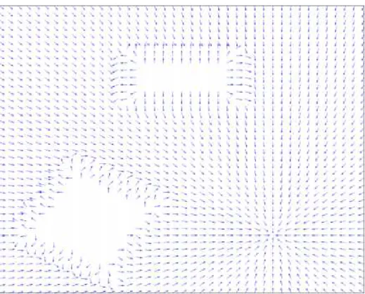
Figure 3.1 shows a discretized work space with the associated potential field. The major concern while working with potential functions is the selection of a differentiable real-valued functionU:Rn→R. The functionU is illustrated in Figure 3.1d. At any given
as the energy of the moving particle at that point. By measuring the negated gradient of the potential functionU, the force applied to the particle at any given point can be calculated and by assigning the value of the negated gradient −∂U
∂x and −
∂U
∂y to any point on the
workspace the vector field is generated. This generated vector field would direct any particle from any given start point towards the predefined goal point. An intuitive metaphor to understand this algorithm is to consider the 2-D rigid body of the robot as one single point in the configuration space where according to the position of this particle a specific force drives the point towards the goal.
Generally it is considered that the robot mass point is a positively charged particle and the goal configuration is considered to be negatively charged, and thus pulling the robot towards itself. While the obstacles are positively charged, pushing the robot away from the C-Space obstacle. The combination of attractive and repulsive potentials create this force field. As illustrated in Figure 3.2 on page 19 if we consider the robot as a point, it will follow a path downhill towards the goal point, regardless of where the starting configuration is located.
One of the points that make potential fields very interesting is that, this method can be used as a feedback motion planner for any mass point robot. At any given point there is a vector directing the robot towards the goal, so the controller should only have to control the heading of the robot and make sure it follows the right direction. The reference to the controller is the heading, and it could be easily controlled using a PI controller. By con-structing a feedback control plan over this continuous space we could generate a trajectory and use trajectory tracking methods and to track it. This would make potential functions a closed loop feedback motion planning algorithm. As shown in Figure 3.2 on page 19 for all points in the work space there is a vector defined that could direct the robot towards the goal.
As intuitive and as simple as this method is, it has its own draw backs. Consider the case where the potential function introduces a local minima to the potential field, due to the geometry of the obstacles or simply due to the position of the obstacle relative to the goal. In this case if the starting configuration is close enough to this minima, or the path passes close
(a) A Work Space with two rectangular obstacles
(b) Attractive potential field (c) Repulsive potential field
(d) Total potential field
Figure 3.2: Negated gradient vector field
by this local minima, the robot might get trapped in the local minima and will never rich the goal. There are different potential functions other than the attractive/repulsive potential, but almost all of them suffer from the same problem, which is the existence of local minima. That’s why potential functions are not considered as a complete motion planner.
3.2
Potential field for
C
=
R
2The function defined below was introduced by Khatib [18] and it is probably the most famous potential function for mass point robots inR2and evenR3. Let’s first construct the
artificial forces applied to a point in R2. The potential should be a differentiable function, U :C → R. The artificial forces can be easily found by finding the negated gradient vector:
~
F(q) =−~∇U(q) (3.1)
since we are working with just a point the configurationqdoes not consider the orientation of the robot, θ. The total potential function is constructed as the sum of the attractive and repulsive potential functions:
U(q) =Uatt(q) +Urep(q) (3.2)
3.3
Attractive potential
The role of the attractive potential is to drive the robot to the goal configuration. Maybe the simplest function that could play the role of the attractive potential is the euclidean distance.
U(q) =Kattd(q,qgoal) (3.3)
the value of the function is always positive and somehow represents an error, the distance between current configuration and the desired configuration. This function only has one global minimum at the goal configuration where the potential is zero. The gainKatt is used
to change the effect of the attractive potential function. If the gain is higher the attractive potential will be higher. The gradient of Equation (3.3) is
∂U(q) ∂x = Katt(x−xgoal) d(q,qgoal) ∂U(q) ∂y = Katt(y−ygoal) d(q,qgoal) (3.4)
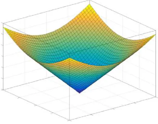
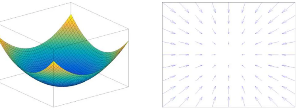
Selecting this gradient function results in a linear change in the force exerted on the robot and when implemented it will result in a non-smooth motion. Also as illustrated in Figure 3.3 on the next page the gradient is not defined ifq=qgoal and the function becomes non-differentiable. We can simply use a quadratic potential function instead of the conic potential function to have a smooth differentiable function.
Uatt(q) =
1 2Kattd
2(q,q
Figure 3.3: Conic potential field
and the gradient would be
∂Uatt(q)
∂x =Katt(x−xgoal) ∂Uatt(q)
∂y =Katt(y−ygoal)
(3.6)
The quadratic potential function also provides a smooth vector field as the robot ap-proaches the goal. When the robot is far away from the goal, the gradient has a higher value and as the robot approaches the goal the gradient decreases. The 12 fraction is added to simplify the gradient function. As it can be seen in Figure 3.4 on the following page the quadratic potential function is smooth and differentiable.
Figure 3.4: Smooth & differentiable attractive potential field
3.4
Repulsive potential
The repulsive potential helps the robot stay away from the obstacles or the work space boundaries. Also it is desirable that the the robot does not get under the influence of the obstacles when it is far from them. It is also assumed the obstacles are convex, if they are not some decomposition algorithm must be used to make all obstacles convex. Equation (3.7) encapsulates this concept. For each obstacleCOithe distance functionDi(q)is the distance
between the current location of the robot to the closest point on the obstacle.
Urep,i(q) = 1 2Krep( 1 Di(q)− 1 D∗), ifDi(q)≤D∗i 0, ifDi(q)>D∗i (3.7)
D∗i is the threshold distance and represents the range of influence of obstacle COi{}. It is interesting to note that this threshold distance is not necessarily similar for all obstacles and it can have different values according to the type of the obstacle. Just like theKatt, the effect of the repulsive function could be tuned using a gainKrep. As the distance between
the robot and obstacleCOi is decreased the value of the potential function is increased and tends to infinity.
The total repulsive potential field is obtained by adding the effect of all obstacles. Givennobstacles the total potential field is
∇Utotal=∇Uatt+ n
∑
i=1 ∇Urep,i Ftotal =−∇Uatt− n∑
i=1 ∇Urep,i (3.12)Once the vector field is constructed there are different approaches on how to use this vector field and drive the robot towards the goal [22].
• Consider the vector field as a vector of generalized forces that make the robot move in a certain way according to the current configuration of the robot and the dynamic model of the robot
τ=Ftotal(q) (3.13)
• Consider the vector field as a velocity field which describes the velocity of the robot in the configuration space
˙
q=Ftotal(q) (3.14)
In this thesis we only deal with the kinematic model of a robot, so the second ap-proach is more attractive. Once the desired velocity of the robot in the configuration space is known, the robot could be controlled using the kinematic model and Equation (3.14) pro-vides the reference velocity to the controller. The motion planner does not have to provide a trajectory, i.e. a profile of the velocity or acceleration along the path, so it is logical to assume a constant velocity along the path. So, to make things easier it’s usually assumed that the final vector field is normalized.
3.5.1
Continuous motion planning
As it was mentioned before, it is assumed the system is a point in the working space and thus there are no constraints on the system. So, the representation of the system is ˙x=
1. A worldW, obstaclesO, robotA, and configuration spaceC
2. An input spaceU
3. A state transition equation ˙q=−u
4. An initial configurationqinit∈ Cf reeand a goal setqgoal⊂ Cf ree
the motion planner should return a set of waypoints from the initial configuration to the goal configuration. The input spaceU, is actually the total vector field over the workspace. Notice that the the goal configuration must be a set of valid configurations. Usually it is reasonable enough to accept a path which makes the system get close enough to the goal. To find the way points the most common choice is the simple numeric integration of state transition equation using the Euler method
qi+1=qi−αU(qi) (3.15)
Equation (3.15) could also be considered as the gradient descent algorithm. Once the initial configuration is known, the robot would move step by step in the direction guided by the force field, which is the negated gradient of the potential field. The only tricky part of this algorithm is selecting how fast the robot should move towards the goal. If the steps that the robot is taking are too big, the robot might pass the goal and/or oscillate around the goal configuration. On the other hand if the steps are too small, it might take a long time for the robot to reach the goal [5].
Algorithm 1Gradient Descent
q(0)=qstart i=0 while∇Utotal(q(i))6=0do q(i+1) =q(i)−α∇Utotal(q(i)) i=i+1 end while
The input of the algorithm is the start configuration, a function to calculate the force field related to the current stateq(i)and some scalar coefficientα, which decided how far at each step the robot should proceed. The larger this coefficient, the larger the step. It is worth mentioning thatα is not necessarily a constant, and it could be dynamically changed. A good approach for changingα is to select a larger value at the beginning and as the robot gets closer to the goal decrease the coefficient [5]. Also, it is almost impossible for the condition ∇Utotal(q(i))6=0 to ever become true. So a more relaxed condition is usually
used k∇Utotal(q(i))k<ε, where ε is selected based on the condition of the task at hand,
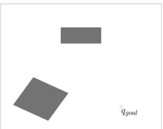
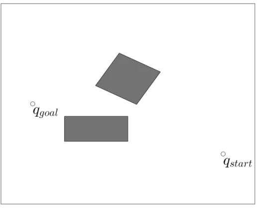
the smaller theε the closer the robot will be to the goal. That is why the goal configuration is a set rather than a single point. Consider the working space illustrated in Figure 3.6. The goal is to plan a path fromqstart toqgoal.
Figure 3.6: A work space with rectangular obstacles
Figure 3.7 shows the planned path using simple gradient descent with a constant step size α =0.2. But as it can be seen there are a lot of oscillations in the generated path. Unfortunately these oscillations are one of the negative points about potential functions.
U(q+∆q) =U(q) +b(q)T∆q+1
2∆q
TA(q)∆q (3.18)
whereb(q)is the gradient of the potential function andA(q)is the Hessian matrix calculated at q. Equation (3.18) will be minimized by the solution to A(q)q=b. As proved here [33] the value of theα which minimizes equation Equation (3.18) can be calculated using equation Equation (3.19)
α = r
Tr
rTAr (3.19)
where the residualr=b−Aqshows the error between the correct value ofband its’ esti-mated value. Onceα is calculated the following algorithm is used to update the state of the system
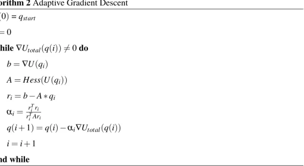
Algorithm 2Adaptive Gradient Descent
q(0)=qstart i=0 while∇Utotal(q(i))6=0do b=∇U(qi) A=Hess(U(qi)) ri=b−A∗qi αi= r T iri rT iAri q(i+1) =q(i)−αi∇Utotal(q(i)) i=i+1 end while
Figure 3.8 shows the same work space as the one in Figure 3.6 but the path is gener-ated using Algorithm 2. Although the genergener-ated path is much smoother and there are not that many oscillations, but we have to realize what we are giving to gain this smoother path. In the simple gradient descent algorithm we only had to calculate the gradient and we had full control of the step size α, but here not only we have to calculate the hessian matrix at any given point but we also have to deal with the conservative nature of this algorithm
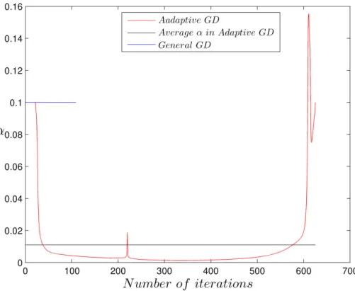
which chooses much smaller time steps. Figure 3.9 shows a comparison of the value of the step size in the two different methods. As it can be seen the normal implementation of Euler method, general gradient descent, has much less number of iterations, around 150. But The adaptive gradient descent algorithm has gone through around 650 iterations to converge to the goal point. It is an obvious observation when you consider how small the step sizeα is for a large section of the adaptive algorithm. The average value ofα in adaptive algorithm is 0.011 while the constant step size foe the general gradient descent algorithm is 0.1 which is almost 10 times larger. For cases where the normal gradient descent algorithm has a hard time converging to the goal or there are a lot of oscillations it might be better to use the adaptive gradient descent algorithm.
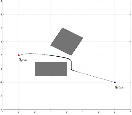
Figure 3.8: Planned path by updatingα at each iteration
But this won’t stop us from using adaptive gradient descent. Actually the main reason for using gradient descent is cases where the normal gradient descent algorithm does/can not converge to the goal. Consider the same work space illustrated in Figure 3.10 which
Figure 3.9: Dynamics ofα as a function of number of iterations
is the same as Figure 3.6 but with different locations for the start and goal configurations. Running the general gradient descent algorithm on this problem would not generate a path. As shown in Figure 3.10 there are a lot of oscillations close to the obstacle and the algorithm did not converge even after 4000 iterations. But on the same work space and start/goal con-figurations the adaptive gradient descent algorithm converges and a smooth path is planned. The path is found after almost 1650 iterations.
There are also other algorithms such as conjugate gradient descent, newton’s method and also the momentum gradient descent which can solve this problem. In nature they are very similar to the previously discussed algorithms but they have different running times, number of iterations, and behavior depending on the problem.
So far we have solved one of the big problems of potential functions which is numer-ous oscillations close to the obstacles or between them in a corridor. But there is another challenging problem regarding the potential functions. Consider the work space in figure 3.12, it seems even simpler than the previous work space as there is only one obstacle
Figure 3.11: Planned path by updatingα at each iteration
minima problem. The algorithm is described in Subsection 3.5.3, discrete motion planning.
• Rimon and Koditschek [32] developed an analytic method to find a special family of potential functions calledNavigation Functionswhich just like potential functions would result in a velocity field but there are no spurious local minima and there is only a single minimum located at the goal. Maybe the most distinctive property of such potential functions is that they must be a Morse1 [28] function to satisfy the single global minimum criteria. A Morse function is a function where all critical points the Hessian are nondegenerate. Just like the potential functions this method assumes a repulsive force from the obstacles and an attractive force from the goal. This method is also described in Subsection 3.5.2
• Connolly et. al. [8] proposed a special family of navigation functions which are numerical solutions to Laplace’s heat equation and they are usually calledHarmonic
(a) Even a simple work space can have the local minima problem
(b) The potential function contour over the workspace exposing local minima
Figure 3.12: Local minima in a workspace when the direction of movement is perpendicular to one of the obstacles in the workspace
Potential Functions. Harmonic potential functions hold all conditions for a navigation function except being aMorsefunction due to the possibility of isolated degenerate saddle points.
A functionφ is called a harmonic function if it satisfies the differential equation
∇2φ = n
∑
i=1 ∂2φ ∂x2i =0 (3.20)Usually finite element methods are used to solve for the solution of Equation (3.20). In order to solve the equation one must define some conditions on the boundary of the domain over which the functionφ is defined. Usually eitherDirichlet boundary conditionor Neumann boundary condition or a superposition of the two conditions is used depending on the work space. Here lies one of the problem with Harmonic potential functions, they require an explicit boundary of the free spaceCf ree and it’s
usually avoided in path planning algorithms. Also the numerical solution might be feasible in low dimensions but in higher dimensions it is expensive [22].
Figure 3.13: There is no deterministic gradient descent algorithm to solve the local minima problem
they use cell decomposition and make convex polygons in the free space Cf ree and
build a vector field and define a control policy on each single cell and a switching strategy to smoothly switch between control policies of each cell. Choset et al have used theHarmonic potential functionto create this vector field but Lavalle has pro-posed a very interesting approach where they creates the vector field directly without having to define a potential function based on the distance of edges and vertices to the current location of the robot.
3.5.2
Navigation functions
The major concern with potential functions is the existence of local minima. One of the methods that tries to construct a feedback motion planner over the continuous free space is called Navigation Functions which have been proposed by Rimon and Koditschek [32].
(a) A vector field is constructed directly with-out a potential function
(b) Trajectories from different initial condi-tions to the goal
Figure 3.14: Lavalle et. al. [25] proposed an algorithm to use cell decomposition and create convex cells and then construct the vector field directly on each cell
Figure 3.15: Choset et. al. [6] used the weak harmonic potential functions on decomposed cells
They have showed that it is not possible to construct a scalar field free from critical points. But they proposed a set of functions which construct a globally asymptotic scalar potential filed in which the critical points are unstable (i.e. the Hessian is non-singular and the critical point is non-degenerate). Thus, in implementation it is practically impossible for the point-mass robot to get trapped in such unstable critical points.
In the proposed method the motion planning algorithm is abstracted from the geomet-ric space to a topological space, usually this topological space is called a ”model space”. The obstacle avoidance problem is then equivalent to staying in the same connected section of the free space Cf ree, in which the point-mass robot has started. The model space could
be considered any generalized sphere world.
For cases where the obstacle and the work space are not a sphere, a diffeomorphism is used and the geometric complicated obstacles are mapped into simple sphere in the model space. Then a navigation function is constructed on the model space, the motion planner generates a path and then the inverse of the diffeomorphism is used to transform the path from the model space to the real work space. In Subsection 3.5.2.1 the simpler sphere world is considered where there is no need to have a diffeomorphism because every thing is already a simple Euclidean sphere. Then in Subsection 3.5.2.2 a more general and com-plicated geometry of the work space is considered and it is described how to define the diffeomorphism and its inverse.
3.5.2.1 Navigation functions in a sphere world
A sphere world is defined as a compact, close and bounded, subset of n-dimensional eu-clidean space En whose boundary is a single (n−1)−dimensional sphere. In this thesis
however only the 2-dimensional euclidean space is considered. The space bounded by this 1-sphere called theworkspaceW and is defined as
W={q∈E2| kqk26ρ02} (3.21)
bounding sphere is considered to be at the origin. If there are a total of M obstacles in the working space the number of all spheres would beM+1, where the extra 1 is the outer sphere. The remainingMother spheres which bound the obstacles present in the workspace are defined as
Oj={q∈E2| kq−qjk2<ρ2j}, j={1,2, ...,M} (3.22)
whereqjis the center of each spherical obstacle and its radius isρj>0. Thus the configu-ration space obstacleis defined as
Cobs= M
[
j=1
Oj (3.23)
the free space remains after removing all obstacles from the workspace
Cf ree=W \ Cobs (3.24)
Notice that according to the definition ofconfiguration space obstaclethe boundary of all obstacles are in the free space thus it would be a valid path if the point-mass robot goes on this boundary, which in reality represents scratching the surface of an obstacle. One could assume the workspace as a standard disk and the obstacles as spherical punctures in this disk. This idea is represented in Figure 3.16.
The formal definition [5] of a navigation function is as follows :
Definition 3.5.1.
IfCf ree is a compact analytical manifold with boundary then the mapϕ:Cf ree→[0,1] is called a navigation function if it:
1. is analytical onCf ree(Infinitely differentiable, smooth, or at least Ck for k>2) 2. is polar onCf ree(A unique minimum exists at qg∈ Cf ree)
3. is Morse onCf ree(All critical points are non-degenerate)
Figure 3.16: Different sets on a sphere world with respective dimensions
The potential function proposed by Koditschek-Rimon has all of the above mentioned properties1.
The potential that acts as the attractive portion of the navigation function is the simple euclidean distance to the goalγ :Cf ree→[0,∞)
1They have also proved that all critical points appear close to the boundary of the free spaceC
f ree. They
have shown these critical points would vanish from the free space if an annulus with a widthεis added around all obstacles. It is also proved that there is a formulation to find the minimum value forεwhich satisfies this condition
γ(q) =γgk(q), k∈N\ {0,1}; γg(q) =kq−qgk2 (3.25)
whereγ is zero at the goal configuration and increases as q moves away from the goal. The repulsive portion is the product of obstacle functions present in the workspaceβ :Cf ree→
[0,∞) β(q) = M
∏
j=0 βj(q) (3.26)whereβjs are defined as
β0(q) =ρ02− kqk2; βj(q) =kq−qjk −ρ2j, j=1,2, ...,M (3.27)
the definition of obstacle functions is direct result of the way the configuration space ob-stacle is defined. The outer sphere which constructs euclidean disk is considered a s the zeroth Obstacle. According to Equation (3.27) the obstacles hold a negative value inside the obstacle, zero on its boundary and positive in the free spaceCf ree. Also notice the same
thing holds true for β(q) as it is the product of the obstacles and not the summation of the obstacles, in contrast with the way repulsive potential was defined in Khatib’s potential function.
Using the repulsive and attractive potentials the function ˆϕ(q) = βγ((qq)) is defined. Asq
approaches the boundary of any obstacleβgoes to zero and ˆϕgoes to infinity thus repelling the robot. Also it is only zero at the goal configuration, whereγ is zero. As [ref to Robot Navigation Functions on Manifolds with Boundary theorem 4] Koditschek-Rimon have proved there exists a positive integerNsuch that for everyk>N, ˆϕhas a unique minimum at the goal configuration. It is very easy to see that in ˆϕ, as k increases the numerator changes more significantly compared to the denominator and thus ˆϕpoints toward the goal. It is also worth mentioning that the critical points also move closer to the boundary of the obstacles as k increases because the effect of repulsive function from the obstacles is reduced in further distances [19].
Asq approaches the boundaries ˆϕ can have arbitrarily large values. So the diffeo-morphismσ :[0,∞)→[0,1]is introduced to bound ˆϕ
σ = x
1+x (3.28)
this diffeomorphism maps the range of ˆϕ to the unit interval. Using this diffeomorphism the values at the boundary of any obstacle is 1 and the goal has a value of zero. But with someks it might have a degenerate critical point at the goal. So a distortion is introduced to eliminate the degeneracyσd: [0,1]→[0,1]
σd(x) =x
1
k; k∈N (3.29)
the final function which poses all the conditions of a Navigation Function will be
ϕ= (σd◦σ◦ϕˆ)(q) =
γg(q)
(γ(q) +β(q))1k
(3.30) which is guaranteed to have a single unique minimum atqgifkis sufficiently large.
Consider the workspace depicted in Figure 3.17 on the following page. We would like to construct a scalar potential filed on the free space of this workspace. Then use the gradient descent algorithm to find a path starting from any point in the free space toward the goal qgoal. As discussed earlier such a potential field can be constructed using
Equa-tion (3.30). Figure 3.18 shows how this scalar field develops as the parameterkis increased. Notice that the existence of local minima is apparent wherekholds a smaller value but ask
increases the scalar field changes and after a large enoughkthere is no local minima in the free work space.
Figure 3.19: Change in the scalar field over free space asKincreases
Figure 3.20 shows different paths with different with different initial positions. For this configuration the gainK is set to 7. As it can be seen all the paths are collision free. evolves starting from different positions towards the goal.
3.5.2.2 Navigation functions in a star world
In the previous section it was assumed that we are in a perfectly defined Euclidean Sphere World. This section tries to solve the path planning problem in a more general world, aStar World. Let’s first mathematically define a Star shaped world. In set theory a star shaped setSis a set where there exists at least one point in the set that is within line of sight ofall
other points of the same set: The construction of analytic diffeomorphisms for exact robot navigation on star worlds [5]:
∃xsuch that∀y∈S, tx+ (1−t)y∈S ∀t∈[0,1] (3.31)
In the same spirit an obstacleOj is considered Star Shaped if there is a pointqj∈ Oj such
that for allq∈ Ojthe inward gradient∇βj(q)satisfies
∇βj(q).(q−qj>0 (3.32)
if all obstacles in the free space,Sf ree, are star shaped then,Sf reeis called aStar World.
In the previous section it was shown how to find a navigation function for Sphere Worlds. With a Star World we should first map the Star World to a Sphere World, solve for the navigation function and then use a diffeomorphism to map the navigation function back to the Star World.
Thinking about the definition of aStar World you might realize how close they are to aSphere World. ASphere Worldcould be thought of as a homeomorphism of aStar World
and ice versa [5]. The construction of analytic diffeomorphism for exact robot navigation on star worlds Elon Rimon, Daniel E. Koditschek have shown that given a navigation function in the free configuration spaceP of a Sphere Worldϕ:Pf ree→[0,1]there always exists a
mapping which is a diffeomorphism 2from a Star World to the Sphere World h:Pf ree→ Sf ree.
Rimon and Koditschek have shown that the construction of analytic diffeomorphisms for 2A diffeomorphism is a map between two smooth manifolds. It is an invertible, and thus bijective, map-ping. Both the diffeomorphism and its inverse are smooth
exact robot navigation on star worlds could be achieved in two steps. In the first step the the start world is mapped to a homeomorphic sphere world, then the navigation functions are constructed under the sphere World and then they could be pulled backinto a Star World using this diffeomorphism.
So if ϕ :Pf ree →[0,1]is a navigation function on P and h: Pf ree → Sf ree is the
analytical diffeomorphism then
φ :ϕ◦h. (3.33)
is a navigation function on theStar WorldS. The bijective property of the diffeomorphism guarantees that there is a one-to-one relation between the critical points and obstacles.
3.5.3
Discrete motion planning
As discussed in the previous sections, although the potential function idea is very elegant and simple but it has one major draw back which is the existence of local minima, let alone the oscillations which generally could be solved using the right selection ofαi. There is no
simple deterministic algorithm to solve the local minima problem other than the Navigation functions. They provide very beautiful and elegant solution for this problem but at the same time they add a lot of complexity to the the problem. Even a simple work space needs a lot of work to implement the navigation function. But there is a special type of Navigation Functions on spaces which are represented as grids called WaveFront Planner. These family of navigation functions are probably the simplest solution to the local minima problem and are used in a lot of different motion planners and also a lot of video games as the algorithm is very easy to implement and work with. The input to the WaveFront planner is an occupancy grid3. Occupancy grids were first popularized by Hans Moravec and Alberto Elfes at CMU. As our initial assumption about the workspace he occupancy grid used in this thesis is a binary map, 0 or 1. Because we have assumed we have perfect mapping information about 3An occupancy grid is a discrete probabilistic method to represent a work space. Each cell holds a proba-bility value that shows the certainty if that cell is occupied or not. 1 shows a 100% certainty of an obstacle on that cell and 0 shows a 100% certainty that it is a cell free of obstacles
the workspace. Figure 3.20 shows a Work Space and its corresponding occupancy grid.
(a) A simple work space (b) Occupancy grid
Figure 3.20: (a) Shows a simple work space with 2 rectangular obstacles and (b) Shows the occupancy grid representation of the same work space. Cells that lie on an obstacle have a value of 1 and the free cells have a value of zero
The goal cell has a value of 2. The wave Front planner starts from the goal, then finds all zero valued cells around the goal and change their value to 3. In the next step all zero valued cells adjacent to cells with a value of 3 are update to have a value of 4. This process continues until the whole gird is covered. The value of a cell holds could be interpreted as a cost function, the cost it takes to move from the goal cell to the current cell. The wave front algorithm is described below
Algorithm 3Wave Front Algorithm
Label the goal cell in the occupancy grid with a 2 i = 2
Find all zero valued cells neighboring the cell with value i Update the label for all the zero valued cells to i+1
i = i+1 Go to step 3
The only question that remains unanswered is how the neighboring cells are found. Consider Figure 3.21 where two types of possible neighborhoods are shown. If the dynam-ics of the robot allows movements in diagonal direction usually the 8-neighborhood method is chosen and the cellMhas 8 children in the graph induced by Moore connectivity. If the movement of the robot is limited the 4-neighborhood method is chosen and the cellM has 4 children in the graph induced by the Von Neumann connectivity.
(a) Von Neumann connectivity inducing 4-neighborhood for the central cell
(b) Moore connectivity inducing 8-neighborhood for the central cell
Figure 3.21: Comparing a 4-neighborhood and an 8-neighborhood connectivity
Figure 3.22 on the following page shows how the wave front planner grows on the work space shown in Figure 3.20 if the 8-neighborhood connectivity is chosen.
As it might not be clear how the wave is propagating through the workspace Figure 3.23 shows the same wave propagation where the cells having similar colors also have the same cell value.
Once the wave front has expanded all the cells in the grid, a simple gradient descent algorithm can be implemented to find a path from any given start point towards the goal. That is a very positive point about Wave-Front algorithm. For a given work space and static obstacles the algorithm runs only once but it will work for any start configuration in the free work space. That’s why a lot of researchers categorize this algorithm as a Feed Back motion planning algorithm because a new control input is provided based on the last position of the system. The accuracy of this algorithm depends on how small each cell is. On the other hand the smaller the size of a cell, the longer it would take for the algorithm
Figure 3.22: Wave front planner growing inside a workspace
to go through the whole grid. Figure 3.24 shows the final path generated using the gradient descent algorithm starting from an arbitrary configuration.
Figure 3.23: Wave front planner growing inside a workspace different colors represent different cost of a cell
(a) A path found using gradient descent on the wave front grid
(b) The same path on the work space created by connecting gray cells on the grid
Figure 3.24: A path found using gradient descent is shown on the grid, and the same path is shown on the work space
Chapter 4
Heuristic-Based Path Planning
In this chapter the basic terminology and mathematical background necessary to understand graphs is covered. This first part will give enough intuition to introduce search algorithms and then discuss and compare their differences.
4.1
Graph basics
In heuristic-based Path Planning the problem is usually represented as a graph and then a graph-searching algorithms is used to solve the path planning problem. Such search algo-rithms have been used extensively to solve different engineering problems such as routing of telephone traffic, navigation through mazes, layout of printed circuit boards, etc. In gen-eral there are 2 main different approaches to solve a graph-search problem, mathematical approach and heuristic approach. The mathematical approach usually considers the ab-stract properties of a graph rather than the computational feasibility of the solution while
heuristic approachesusually use a special knowledge about the domain of the problem to improve the efficiency of the solution.
A graph, in the most common sense, is an ordered pairG= (V,E)such thatV is a set of vertices{vi}, or nodes, andE is a set of edges{ei j}, or arcs. In such a graph each edge is related with two distinct vertices. If emn is an element form the set of edges then there
{(0
![Figure 2.1: Geometry of a generic differentially driven robot [22]](https://thumb-us.123doks.com/thumbv2/123dok_us/607649.2572784/19.918.395.582.108.347/figure-geometry-generic-differentially-driven-robot.webp)
![Figure 2.2: A visualization of Configuration Space for a double pendulum [5]](https://thumb-us.123doks.com/thumbv2/123dok_us/607649.2572784/23.918.305.671.355.470/figure-visualization-configuration-space-double-pendulum.webp)