Effective techniques for handling incomplete data using decision trees

(1)

Open Research Online

The Open University’s repository of research publications

and other research outputs

Effective techniques for handling incomplete data using

decision trees

Thesis

How to cite:

Twala, Bhekisipho E.T.H. (2005). Effective techniques for handling incomplete data using decision trees. PhD thesis The Open University.

For guidance on citations see FAQs.

c

2005 The Author Version: Version of Record

Copyright and Moral Rights for the articles on this site are retained by the individual authors and/or other copyright owners. For more information on Open Research Online’s data policy on reuse of materials please consult the policies page.

(2)

31 0287909 5

11111111 II

EFFECTIVE TECHNIQUES FOR HANDLING

INCOMPLETE DATA USING DECISION TREES

A DISSERTATION

SUBMITTED TO THE DEPARTMENT OF STATISTICS AT THE OPEN UNIVERSITY, MILTON KEYNES

IN FULFILLMENT OF THE REQUIREMENTS FOR THE DEGREE OF

DOCTOR OF PHILOSOPHY

By

Bhekisipho ETH Twala

January 2005

(3)

©

by

(4)

This thesis is dedicated to the memories of my dad and three sisters -Bhekithemba (1929-2002) Zanele (1966-1997), Hlengiwe (1971-1997) and

(5)

Abstract

Decision Trees (DTs) have been recognized as one of the most successful formalisms for knowledge representation and reasoning and are currently applied to a variety of data mining or knowledge discovery applications, particularly for classification problems. There are several efficient methods to learn a DT from data. However, these methods are often limited to the assumption that data are complete.

In this thesis, some contributions to the field of machine learning and statistics that solve the problem of extracting DTs for learning and classification tasks from incomplete databases are presented. The methodology underlying the thesis blends together well-established statistical theories with the most advanced techniques for machine learning and automated reasoning with uncertainty.

The first contribution is the extensive simulations which study the impact of missing data on predictive accuracy of existing DTs which can cope with missing values, when missing values are in both the training and test sets or when they are in either of the two sets. All simulations are performed under missing completely at random, missing at random and informatively missing mechanisms and for different missing data patterns and proportions.

The proposal of a simple, novel, yet effective proposed procedure for training and testing using decision trees in the presence of missing data is the next contribution. Original and simple splitting criteria for attribute selection in tree building are put forward. The proposed technique is evaluated and validated in empirical tests over many real world application domains. In this work, the proposed algorithm maintains (sometimes exceeds) the outstanding accuracy of multiple imputation, especially on datasets containing mixed attributes and purely nominal attributes. Also, the proposed algorithm greatly improves in accuracy for 1M data. Another major advantage of this method over multiple imputation is the important saving in computational resources due to it simplicity.

(6)

The next contribution is the proposal of three versions of simple probabilistic techniques that could be used for classifying incomplete vectors using decision trees based on complete data. The proposed procedure is superficially similar to that of fractional cases but more effective. The experimental results demonstrate that these approaches can achieve comparative quality to sophisticated algorithms like multiple imputation and therefore are applicable to all kinds of datasets.

Finally, novel uses of two proposed ensemble procedures for handling incomplete training and test data are proposed and discussed. The algorithms combine the two best approaches either with resampling (REMIMIA) or without resampling (EMIMIA) of the training data before growing the decision trees. Experiments are used to evaluate and validate the success of the proposed ensemble methods with respect to individual missing data techniques in the form of empirical tests. EMIMIA attains the highest overall level of prediction accuracy.

(7)

Acknowledgements

Thanks Lord for making all things possible and for all the blessings you have bestowed on me and my family. With every word on this thesis I give thee praise.

I always considered it trite and over-fulsome of thesis authors to list a full set of people who were 'invaluable'; always, that is, until I wrote a thesis and realised just how deeply I am in debt to the people listed below.

First and foremost, credits and very special thanks to my supervisor, Chris Jones, for willing to take a chance with me and making this venture a reality, and without whom this thesis would not have been possible. Writing this thesis was a blast. Our concept from the beginning was to prepare a thesis that was different and fun writing it. I feel like we succeeded on both counts. You are a master, as in academia ... so in life!!! To thank you in perpetuity for all that you have done for me, I proudly name the principal construction of this thesis - the CMJ series - after you.

To David Hand, sincerest thanks for your great talents, instinct, constant patience, ideas, suggestions and great mind - it is indeed a pleasure to know you. Additional special thanks and great appreciation to Allan White for your tremendous help, thoughtful commentary, practical advice and for forcing me to think on my feet - it has been both enlightening and entertaining!!! I am also thankful to Wray Buntine for giving me a solid start, especially for encouraging me to learn about implementation properly; and as I do theory, whip up a quick implementation to back up things ... hence, in part, bringing that magic to research.

I would like to express my thanks to the Open University for giving me an opportunity to do such a research I can be proud of and for contributing to a research environment that has proven immensely rewarding. To all the members and staff of the Statistics Department at the Open University - it never ceases to amaze me how much the unique and incredible talents of each individual contribute to a thesis. That helped bring this endeavour to life, thank you. I also thank all the members of the 'Thunder Birds Team' (TBT). There will probably never be a time where the

(8)

technology involved when writing a thesis will be snag free. I am so grateful that it is you guys that deal with it instead of me!!!

Much love and respect to my officemates and "sisters", Mona Kanaan and Jane Warwick (at least you can now think in S-PLUS!!!) for putting up with me for almost three years, and for enriching my life immeasurably simply by being such interesting and diverse people.

It gives me great pleasure to thank Martin Shepperd and Michelle Cartwright for your endless patience and goodwill and in letting me finish this project.

Several teachers of statistics have influenced me profoundly at pivotal moments in my early education. I wish to thank Antoni Szubarga for teaching me that the essence of statistics is ideas - not notation!!! I still refer to the copy of M.H. Degroot's book on "Probability and Statistics" which you gave me. I also wish to express warm thanks to M.A. Ali for showing me statistics the way it was meant to be done, and whetted my appetite for more. Like my current supervisor, you also gave me extraordinary freedom to pursue my own interests as a graduate student. It is no exaggeration to say that almost all of the results of this thesis are in some respect fruits of the seeds planted during my time at the University of Swaziland, and for this, I owe you a debt of gratitude. Additional thanks to Elkana (Ali) Ngwenya for teaching me by his own shining example that the most important step by far in any statistical problem-solving is finding the right point of view - the point of view that makes things simple!! In retrospect, you introduced me to the "work smarter, not harder" philosophy of statistics on which I have come to depend.

While at Salesian High School, I was fortunate to learn statistics from Eamon Molloy. I thank you for encouraging me to pursue independent research even at this early age, and for fostering my love of statistics for its own sake. Thank you, Eamon, for launching me on the journey of a lifetime. It was a privilege to be in your class and to have access to a statistician with a masters. I would also like to thank the late Fr. Luke Boyle for his generous nature and for nurturing my development as a high school student, and for enriching my life immeasurably.

(9)

Now that I have recounted the entire history of my statistical upbringing, I have the pleasure of acknowledging those who have provided me with the personal foundation which has been so indispensable to my professional life.

First and foremost, grateful thanks to my mom (Siphiwe) and late dad (Bhekithemba) whose love, understanding and bedrock of support has made my academic career possible - without you none of this would have been possible. You have always been the wind beneath my wings. Your patience and understanding with the relentless demands of graduate study will surely earn you a place among the Saints ofthe Ages!!!

Major domos to "my female team" at home; my wife and constant companion Ntonto, and two lovely daughters, Okuhle (00) and Nobhekisipho (NoB) for putting up with me, and for dealing on a daily basis with a crazy husband and dad. However, there certainly is never a dull moment in our house. For the millionth time, thanks for your patient kindness and love, and for never raising an eyebrow when I claimed my thesis would be finished in the "'next two weeks" for nearly two years. You are all my reasons for living. I will always cherish you.

Much love and happiness back to you, each of my sisters and all our relations; and to all my nephews and nieces, wherever you are, "1 love you!!"

Finally, I also remain truly grateful for the wealth of support and talent I shared with so many researchers, friends, and colleagues. Thanks for bringing gourmet dishes to the research table. You are as solid as they come, not only in your craft, but as people.

Is that everyone??

I alone remain responsible for the content of the following, including any errors or omissions which may unwittingly remain.

"Sometimes a scream is better than a thesis."

(10)

2.1.1 Linear Discriminant Analysis 2.1.2 Logistic Discriminant Analysis 2.1.3 The Multinomial Logit Model 2.2 Density Estimation Methods 2.3 Nearest Neighbour Methods 2.4 Support Vector Machines 2.5 Artificial Neural Networks 2.6 A 'NaIve' Bayes Classifier 2.7 Rule Induction 2.8 Decision Trees 1 3 5 8 8 9 10 10 11 11 14 16 17 19 21 22 24 25 27 29 31 33

(11)

2.8.1 Splitting Rules

2.8.1.1 Information Gain Measure 2.8.1.2 Gain Ratio Measure

2.8.1.3 The GINI Index of Impurity 2.8.1.4 Chi-Square Statistic

2.8.1.5 Normalised Information Gain 2.8.1.6 Other Splitting Measures 2.8.2 Stopping Rules 2.8.3 Pruning Rules 2.8.3.1 2.8.3.2 2.8.3.3 2.8.3.4 2.8.3.5 2.8.3.6

Minimum Cost Complexity Pruning Pessimistic Pruning

Minimum Error Pruning Reduced Error Pruning Error-Based Pruning Other Pruning Procedures 2.8.4 Classification and Error Rates 2.8.5 Decision Tree Algorithms

2.8.5.1 2.8.5.2 2.8.5.3 2.8.5.4 2.8.5.5 2.8.5.6 2.8.5.7 ID3 C4.5 See5/C5.0 CART Other Systems Further Systems

Strengths and Weaknesses of Decision Tree Methods

40 42 43 44 46 46 48 49 49 50 52 51 53 52 53 55 57 59

60

62 63 64 67 70

(12)

CHAPTER 3 MISSING VALUES

3.1 Overview and Problems Caused by Incomplete Data 3.2 Type of Missing Data Mechanisms

3.3 General Approaches to Dealing with Missing Data 3.3.1 Ignoring and Discarding Data

3.3.1.1 Listwise Deletion 3.3.1.2 Pairwise Deletion 3.3.1.3 Re-weighting 3.3.2 Imputation Techniques

3.3.2.1 Single Imputation Techniques 3.3.2.1.1 Mean or mode imputation 3.3.2.1.2 Hot deck imputation

3.3.2.1.3 Regression-based imputation 3.3.2.1.4 Expectation maximization

3.3.2.1.5 Full information maximum likelihood 3.3.2.1.6 Other single imputation techniques 3.3.2.2 Multiple Imputation

3.4 Decision Trees and Missing Data 3.4.1 Imputation Techniques

3.4.1.1 Single Imputation Techniques 3.4.1.1.1 Mean or mode imputation

3.4.1.1.2 Conditioning on class imputation 3.4.1.1.3 ''New'' category level

3.4.1.1.4 Attribute value matching imputation 3.4.1.1.5 All possible values imputation

73 73 75 81 81 81 82 83 84 85 85 86 87 88 91 93 94 97 98 98 98 98 98 100 100

(13)

3.4.1.1.6 Unordered decision tree imputation 3.4.1.1.7 Ordered decision tree imputation 3.4.1.1.8 Bayesian imputation

3.4.1.2 Multiple Imputation 3.4.2 Machine Learning Techniques

3.4.2.1 Surrogate Variable Splitting 3.4.2.2 Fractioning of Cases

3.4.2.3 Dynamic Path Generation 3.4.3 Other Methods 110

CHAPTER 4 EXPERIMENTS WITH CURRENT METHODS

4.1 Introduction 4.2 Related Work

4.3 General Experimental Set-Up 4.3.1 Datasets

4.4 Experimental Results

4.4.1 Overall Results - Incomplete Training and Test Data

4.4.1.1 Results for Individual Data Sets - Incomplete Training and Test Data 101 102 102 104 105 105 108 109 112 112 112 118 128 134 135 140 4.4.1.1.1 Results on a dataset with purely numerical attributes 140 4.4.1.1.2 Results on a dataset with purely nominal attributes 141 4.4.1.1.3 Results on a dataset with mixed attributes 144 4.4.2 Overall Results - Incomplete Training Only

4.4.3 Overall Results - Incomplete Test Data Only 4.4.3.1 Supplementary Experiment and Results 4.5 Discussion

144 148 150 151

(14)

CHAPTER 5 MORE ON THE PROBLEM OF BUILDING DECISION

TREES USING INCOMPLETE VECTORS AND

CLASS~GINCOMPLETE

TREES

5.1 Introduction

VECTORS USING

5.2 Building Decision Trees Using Incomplete Vectors and Classifying Incomplete

Vectors Using Trees - Proposed Procedure 5.2.1 Learning Phase 5.2.2 Classification Phase 5.2.3 Illustration 5.3 Experimental Set-Up 5.4 Experimental Results 157 157 159 159 161 162 165 165

5.4.1 Overall Results - Current Vs. New Methods 166

5.4.2 Results for Individual Datasets - Current Vs. New Methods 168 5.4.2.1 Results on a Dataset with Purely Numerical Attributes 169 5.4.2.2 Results on a Dataset with Purely Nominal Attributes 170 5.4.2.3 Results on a Dataset with Mixed Attributes 171 5.4.3 Current and New Methods: Processing Time

5.5 Discussion

CHAPTER 6 MORE ON THE PROBLEM OF CLASSIFYING

INCOMPLETE VECTORS USING TREES

6.1 Introduction

6.2 Classifying Incomplete Vectors - Proposed Procedure

173 175

178 178 180 6.2.1 The Full Estimation of Probabilities from Training Set 184 6.2.2 Approximation of Probabilities by Related Probabilities Estimated

(15)

6.2.3 The Full Estimation of Probabilities from Training Set Using Binary and Multinomial Logit Models

6.3 Experimental Set-Up 6.4 Experimental Results

188 192 193 6.4.1 Overall Results - Current Vs. New Testing Methods 193 6.4.2 Results for Individual Datasets - Current Vs. New Testing

Methods 196

6.4.2.1 Results on a Dataset with Purely Nominal Attributes 196 6.4.2.2 Results on a Dataset with Mixed Attributes 198 6.4.3 Current and New Testing Methods: Processing Time 199

6.5 Discussion 202

CHAPTER 7 ENSEMBLE METHODS AND DECISION TREES 207

7.1 Introduction

7.2 Combining Missing Data Techniques within the Mechanism of Growing and Testing Decision Trees

7.2.1 EMIMIA Technique 7.2.2 REMIMIA Technique 7.3 Experimental Set-Up 7.4 Experimental Results

7.4.1 Overall Results - Ensembles Vs. Current and Proposed Missing

207 208 208 209 211 211 Data Methods 211

7.4.2 Current, Proposed and Ensembles of Missing Data techniques: Processing Time

7.5 Discussion

CHAPTER 8 CONCLUDING REMARKS

8.1 Research Findings 8.1.1 Current Methods 213 216 218 218 218

(16)

8.1.2 Current Vs. New Methods 221 8.1.3 A Further Idea for Classifying Incomplete Vectors Using Trees 222

8.1.4 Ensemble Methods 223

8.2 Summary of Contributions 224

REFERENCES 226

(17)

List of Figures

1.1 A machine learning diagram 4

1.2 A decision tree framework 4

1.3

An induction learning framework

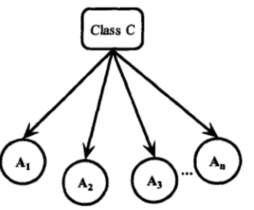
7

2.1 A "naIve" Bayes' classifier 30

2.2 (a) Example of a binary decision tree for a four~dimensional feature

space 37

2.2 (b) Hierarchical partitioning of the two-dimensional space induced by

the decision tree offigure 2.6(a) 37

2.3 The decision tree induction algorithm 39

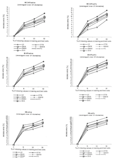
4.1 Effects of missing values in training and test data on the error for

methods over 21 domains 136

4.2 Comparison for training and testing methods: confidence intervals of

mean error rates 137

4.3 Overall means for number of attributes with missing values 137

4.4 Overall means for missing data proportions 137

4.5 Overall means for missing data mechanisms 138

4.6 Interaction between methods and number of attributes with missing

values 139

4.7 Interaction between methods and proportion of missing values 139 4.8 Interaction between methods and missing data mechanisms 139 4.9 Interaction between number of attributes with missing values and

proportion of missing values 139

4.10 Comparative results of methods for the letter dataset 141 4.11 Comparative results of methods for kr-vs-kp dataset 142 4.12 Comparative results of methods for german dataset 143

(18)

4.13 Effects of missing values in training data on the error for methods

over 21 domains 145

4.14 Comparison for training methods: confidence intervals of mean error

rates 146

4.15 Overall means for number of attributes with missing values in training

set 146

4.16 Overall means for missing data proportions (training methods) 146 4.17 Overall means for missing data mechanisms (training methods) 147 4.18 Interaction between number of attributes with missing values and

proportions of missing values in training set 147

4.19 Effects of missing values in test data on the excess error for methods

over 21domains 148

4.20 Comparison for testing methods: confidence intervals of mean error

rates 150

5.1 Standard algorithm for feature selection 161

5.2 A proposed algorithm for feature selection with unknown attribute

values 161

5.3 An artificial example of a simple binary decision tree which allows

'missing' to be a possible choice on the tree 164

5.4 Effects of missing values in training and test data on error of current

and new testing methods 166

5.5 Comparison for current and new methods: confidence intervals of mean

error rates based on pooled standard deviation 167

5.6 Interaction between the number of attributes with missing values and

missing data mechanisms 168

5.7 Comparative results of current and proposed methods for the letter

dataset 169

5.8 Comparative results of current and proposed methods for the kr-vs-kp

dataset 171

5.9 Comparative results of current and proposed methods for the german

(19)

6.1 Example of a binary decision tree from a set of 40 training instances that are represented by three attributes and accompanied by two

classes 183

6.2 Effects of missing values in test data on excess error current and new

testing methods over 21 domains 194

6.3 Comparison for current and new testing methods: confidence intervals

of mean error rates 195

6.4 Comparative results of current and new testing methods for the

kr-vs-kp dataset 197

6.5 Comparative results of current and proposed testing methods for the

zoo dataset 198

7.1 The EMIMIA algorithm 209

7.2 The REMIMIA algorithm 210

7.3 Effects of missing values in training and test data on the excess error

for ensemble and missing data methods over 21 domains 212 7.4 Overall means for current, proposed and ensemble methods 213

(20)

List of Tables

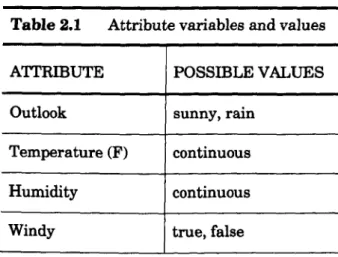
2.1 Attribute variables and values 35

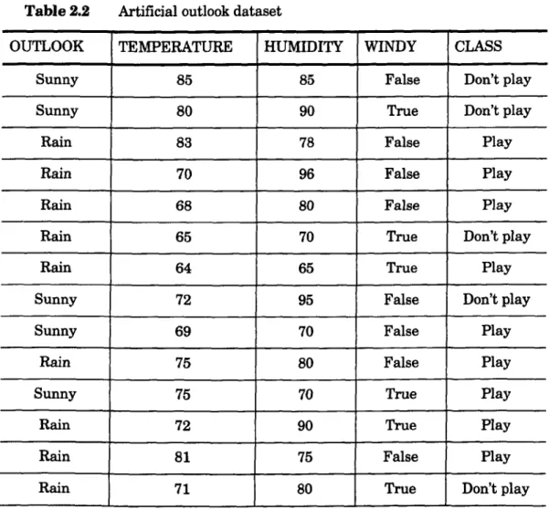
2.2 Artificial outlook dataset 36

3.1 Missing data hierarchy 78

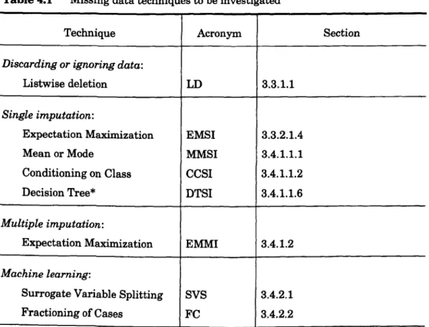
4.1 Missing data techniques to be investigated 119

4.2 Partitioning of dataset to training and test sets 121

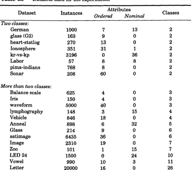
4.3 Datasets used for the experiments 129

5.1 Artificial dataset with missing values on attributes AI and A3 162

5.4 Processing time (in seconds) for current and proposed methods for

selected datasets 174

6.1 Artificial dataset 183

6.2 Processing time (in seconds) for current and proposed testing methods

for selected datasets 201

7.1 An example pattern table 209

7.2 Processing time (in seconds) for current, proposed and ensemble

(21)

Chapter 1

Introduction and Background

Machine Learning (ML), which has been making great progress in many directions, is the hallmark of machine intelligence just as human learning is the hallmark of human intelligence. The ability to learn from observations and experience seems to be crucial for any intelligent being. Likewise, ML plays a central role in Artificial Intelligence research (Holland, 1975; Winston, 1992; Patterson 1996) and has reached a certain level of maturity. It has been heralded as the next revolution in learning systems by some experts in the area--but dubbed an OXYmoron by others. ML is inspired by work in several disciplines. These include computer science, mathematics, psychology, (neuro) biology/genetics, philosophy and among other areas.

Common goals and similar evaluation methods drive ML research. The main aim is to improve performance on some task, and the general approach is finding and exploiting some regularities in training or learning data. The goals driving ML research can be psychological (understanding human learning); empirical (to discover principles relating algorithm characteristics); mathematical (to analyse what concepts are learnable at all); and applications (to use the learning system and results of learning in a real-world situation).

Recently, ML research (Hart, 1984; Michalski, 1986; Forsyth and Rada, 1986; Winston, 1992; Michie et al., 1994; Langley, 1996; Mitchell, 1997; Barry and Linoff, 1997) has begun to payoff in many ways. ML methods are being successfully integrated with powerful performance systems and more established techniques have already made their presence felt. Recent successes in ML and statistics include neural network learning, Bayesian network learning, instance-based or case-based learning, genetic algorithm learning, analytic learning and rule induction, and so on. To date the above could be identified as the six basic ML paradigms under active investigation. These paradigms emerged from different scientific roots; differ in their

(22)

assumptions about the representation, performance and assessment methods, and algorithms used in a learning system. They employ different computational methods, and often rely on subtly different ways of evaluating success, although all share the common goal of building machines that can learn in significant ways for a wide variety of task domains.

ML paradigm techniques are also being applied to new kinds of problems including knowledge discovery in databases, language processing, robot control, and combinatorial optimisation as well as more traditional problems such as speech recognition, face recognition, handwriting recognition, medical data analysis, game playing, discrimination, classification, and so on. Some ML paradigms, like rule induction, which employ decision trees (DTs), are specifically designed to deal with uncertainty and are currently applied in a variety of data mininglknowledge discovery/statistical modelling applications, particularly for classification problems. These are the type of problems that are covered in this thesis.

Classification rules (or classifiers) are used to predict the corresponding class of an example, where the class is some discrete variable of practical importance.

An

application of classification using decision trees is when a bank makes a credit decision or considers giving loans to its customers. This is done by a set of rules that classify each loan applicant as low, medium or high risk, using data collected about previous customers together with if the loans were good, bad or worse. Such rules are called classification rules and the data on old customers is called the training sample of classified cases (training set) from which the classification rules are discovered. These classification rules can then be used to discover the group a new customer belongs to. The main question is whether the objects fall into groups or clusters, as against more haphazardly scattered over the domain of variation.

Despite the success of ML research, there are some problems that currently exist within the ML community. These include bias, overfitting, noise, incomplete data, uncertainty, learning as search, and so on. Some of these problems are discussed briefly in Section 1.3.

(23)

1.1 The Meaning of Learning

To learn means to add something to a body of knowledge, a body that in the extreme might be empty. Learning can be thought of as an interaction between two logically distinct entities, the learner, L, and the supervisor or teacher, T. Learning situations differ in the degree to which the responsibilities of these two entries are functionally separate. The responsibilities of T can be thought of as providing examples or occasions for L, providing a feedback concerning the correctness of L's response to an example and providing a sequence or ordering in which the examples are to be presented to L. The responsibilities of L can be thought of as providing a response or answer to each example presented or modifying its knowledge appropriately based on feedback from T concerning the correctness of its answer. Without learning, everything is new. Hence, it could be argued that a system that cannot learn is inefficient because it re-derives each solution and repeatedly makes the same mistakes.

A learning system uses sample data to generate an updated basis for improved performance on subsequent data from the same source, and expresses the new basis in intelligible symbolic form (Michie et al., 1994). Early attempts to devise learning systems during the cybernetic days of AI proved disappointing, so the whole idea was dropped. Only recently has it been revived. Most, however, would still agree that ML has not lived up to the hype and expectations that began a few years ago even though there have been some advances in this field.

When a computer system improves its performance, without re-programming, it can be said to have learned something. Two of the most central goals of any learning algorithm are to provide more accurate solutions and to cover a wide range of problems that seem to require intelligence, respectively. Other minor goals could be to obtain answers economically and to simplify codified knowledge (Forsyth et al.,

1994).

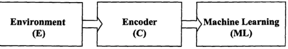
All systems designed to modify and improve their performance share important features. A typical machine learning system does not interact directly with its

(24)

environment. It uses "coded" observations of this environment to learn about it. Fig. 1.1 depicts a framework for a typical machine learning system. The environment E

represents the real world, the environment that is learned about. E represents a finite number of observations, or objects, that are encoded in some machine learning readable format by the encoder C. The set of encoded observations is the training set for the learning algorithm ML.

Environment

Encoder

(E)

(C)

Fig. 1.1. machine learning diagram

Machine Learning

(ML)

Most ML algorithms use a training set of examples as the basis for learning. During the learning phase, the system does not interact directly with its environment (also called a model or a classifier for classification problems), but uses coded observations, often stored in a set of labelled examples - called the training set. The notion of a training set is important in understanding how a machine learning system is tested. Typically there is a database of examples for which the solutions are known. The system works through these instances and derives a rule or set of rules for associating input descriptions with output decisions (Forsyth and Rada, 1986).

The general framework for a tree classifier, Figure 1.2 is a variation of the machine learning framework.

Data Set

(Data Table)

Search Algorithm

(Hill-climbing)

Fig. 1.2. A decision tree framework

Predictive Model

(Decision Rule)

The first step is to select the types of data that will be used by the mining algorithm (decision tree). The search procedure is part of the system that carries out the task.

(25)

It explores the search space defined by a set of possible representations. Associated with each search strategy is the evaluation component or function that can be used to estimate the distance from the current state to the goal state. If these estimates are computed at each choice point, then they can be used as a basis for choice. It is worth mentioning that such a type of framework could apply within different research communities. For an example, statisticians would allow models to be used for estimation purposes (as a search procedure), like, utilising the maximum likelihood (ML) for estimating missing values. Recently, Hand et al. (2001) have

shown how such a framework could apply for data mining.

Two learning techniques are of special interest. In supervised learning, the system searches for descriptions for the user-defined classes (training examples with the correct classification for each example are given). In unsupervised learning the system constructs the summary of the training set as a set of newly discovered classes, together with their descriptions (training examples without classifications are given).

1.2 The Philosophy of Induction

Before discussing further how systems are made to learn it is important that the philosophers' and psychologists' thoughts about the subject be looked at.

Most learning systems are based on the general principle of induction, i.e. the reasoning technique to infer information that is generalised from the information in the database.

Both philosophers and psychologists have formulated laws by examination of several pathological situations caused by multiple comparison procedures (induction). They have looked at the part played by inductive reasoning in knowledge discovery and have attempted to find rational grounds to validate them.

A typical act of induction is one about treatments used in the medical community, whereby scientific evidence comes from clinical trials, but then an induction step is needed to argue that the drug can help people who are not in the trial.

(26)

Another act of induction is the psychic watch repair. A self-proclaimed psychic, Uri Geller, claimed to start previously-broken watches running using his psychic powers. A wonderful story has been heard (though not been able to verify) about how he asked the listening audience of a radio show to place watches on the radio and he would reach out with his psychic powers and start them running. Many listeners then called the station to say that their watches had started to run. However, the number who tried and failed is not known nor the number who could have placed their watch on the radio at another time and had it start running.

Another old favourite is the sunrise "problem"; the sun always rises from the East and set in the West. Never in living memory has anyone seen it do anything else. Throughout recorded history it has always risen in the East and set in the West. Thus, it will do so tomorrow as well.

Hidden prophecies in text is another act of induction. Recent controversy over the book "The Bible Code" has shown that searching over many possible "skip codes" can find apparent hidden messages in any text, not just the bible. Examples are the Microsoft License Agreement and Tolstoy's War and Peace.

Lateral thinking could also be an act of induction, especially to human-problem solving. A good example is of a merchant who owes money to a money lender and agrees to settle the debt based upon the choice of two stones (one black, one white) from a money bag. If his daughter chooses the white stone, the debt is cancelled; if she picks the black stone, the moneylender gets the merchant's daughter. However, the moneylender "fixes" the outcome by putting two black stones in the bag. The daughter sees this and when she picks a stone out of the bag, immediately drops it onto the path full of other stones. She then points out that the stone she picked must have been the opposite colour of the one remaining in the bag. Unwilling to be unveiled as dishonest, the moneylender must agree and cancel the debt. The daughter has solved an intractable problem through the use of lateral thinking.

Even though both acts of induction are of common sense, that does not mean they are necessarily valid - not because the sun would be expected to rise from the West and set in the East or not expect watches to run because of someone's psychic

(27)

powers. Crucial assumptions are needed to justify them. This is one important reason why many philosophers are devoting a lot of attention to the problems of induction these days.

" ... it is the peculiar and perpetual error of human intellect to be more excited by affirmatives than by negatives; whereas it ought properly to hold itself indifferently disposed towards both alike. Indeed in the establishment of any true axiom, the

negative instance is the more forcible of the two" (See Hart, 1984)

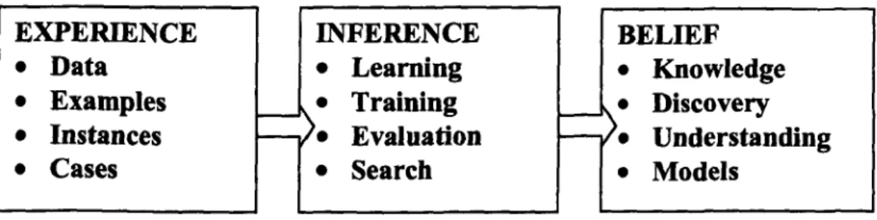
The problem addressed by an inductive-learning system (as shown in Figure 1.2) is to take a collection of labelled "training" data and form rules that make accurate predictions on future data. Inductive learning is particularly suitable in the context of an automated design system because training data can be generated in an automated fashion. For example, one can choose a set of training goals (a training goal is a design goal used for training purposes) and perform an optimisation for all combinations of training goals and library prototypes.

EXPERIENCE

INFERENCE

BELIEF

•

Data

•

Learning

•

Knowledge

•

Examples

_~

•

Training

_{f - -}

•

Discovery

•

Instances

f - - •

Evaluation

I - - •

Understanding

•

Cases

•

Search

•

Models

Fig. 1.3. An induction learning framework

One can then construct a table that records which prototype was best for each training goal. This table can be used by the inductive-learning algorithm to generate rules mapping the space of all possible goals into the set of prototypes in the library. If learning is successful, this mapping interpolates or extrapolates from the training data and can be used successfully in future design sessions to map each new goal into an appropriate initial prototype in the design library.

(28)

1.3 Problems in Machine Learning

There have been a variety of problems that have been the focus of research in the ML community. The most commonly referred to problems shall now be reviewed, even though much work has been spent during the last years to handle them. Also, some of these problems are strongly related to each other, and these relationships have led to considerable attention being devoted to them.

1.3.1 Noise and Overfitting

One problem is that large amounts of data are needed for inductive learning. In many real problems there is a degree of uncertainty or error (imperfection) present in the data. These could lead to errors in the classification process. One source of uncertainty is that of random errors or "noise" which is inevitable. There are many kinds of "noise" that could occur in the examples. These include errors, spurious correlations (Le. correlations that are due mostly to the influences of one or more "other" variables), attributes that are not recorded, two examples having the same attribute/value pairs but different classifications, some values of attributes being incorrect because of errors in the data acquisition process or the processing phase, values of attributes being missing, and the classification or class label being wrong (for example, 1 instead of 2) because of some error. Monago and Kodratofi (1987) present a more detailed analysis of the sources of noise in data.

The next problem is also related to unnecessary attributes (which can be caused by noise) which, besides making no contribution to the predictive performance of the learning system, will simultaneously impose an extra computational burden. This situation is generally referred to as overfitting (Schaffer, 1993; Forsyth et al., 1994;

Cohen and Jensen, 1997), i.e. overfitting the training example data. For example, if the hypothesis space has many dimensions because of a large number of attributes, meaningless regularity maybe be found in the data that is irrelevant to the true, important, distinguishing features. Overfitting is harmful for several reasons. First, overfitted models are incorrect; they indicate that some variables are related when they are not. Second, overfitted models are difficult to understand due to the

(29)

unnecessary component that complicates attempts to integrate induced models with existing knowledge derived from other sources, and overfitting avoidance has sometimes been justified solely on the grounds of producing comprehensible models. Finally, overfitted models can have lower accuracy on new data than models that are not overfitted as demonstrated with a variety of domains and systems by Quinlan (1987).

In the area of decision tree learning, overfitting is avoided or fixed, to a certain extent, by: 1) Termination of tree growth when further splitting the data does not yield a statistically significant improvement or by 2) Growing a full tree, then pruning the tree by eliminating nodes. In practice the latter approach has been more successful.

1.3.2 Missing Values

Another problem that is related to noise is that of incomplete data or missing values. The presence of missing values is commonplace in large real-world databases. This has become one of the most important problems in academic research since most learning systems and statistical analysis were in the early stages not designed to handle missing data (incomplete vectors). There are several reasons why there are missing values in data.

An

item could be missing because it was unavailable or arises by "default" in data recording activities. Missing values could also occur because of confusing questions in the data gathering or because of sensor malfunction. In some situations the missingness could be caused by the relationships between the attribute variables themselves. That is, the information that is missing on a given attribute variable could be as a result of its relation to values of other attribute variables in the data set. An extreme case is that the missing value could be as result of its relation to an unobserved (missing value) in the data set.

Both large and small amounts of missing and/or faulty details in data might mislead the learning process and have an influence in various statistical measures, yet not a lot of work has been done in the research field.

(30)

1.3.3 Bias

The importance of bias has received a lot of attention over the last few years.

By definition, the bias of an estimator is the difference between its mean and the true value. Suppose that there is a function f(x)

=

Y to learn given some sample (X, Y) pairs. There are several hypotheses that could be made about this function. A preference for one hypothesis over the others reveals the bias of the learning system. For example to prefer piece-wise functions or prefer smooth functions or prefer simple functions and treat outliers as noise.

Utgoff (1996) introduced several notions of biases. These are: good bias (which is appropriate to learn the actual concept), strong bias (restricts the search space considerably but is independent of appropriateness), declarative bias (defined declaratively as opposed to procedurally) and preference bias (bias that is implemented as soft preference rather definite restrictions to the search space). Extensions to the problem of bias can be found in Haussler (1988) and Ripley (1996).

In medical statistics bias could define a systematic disposition of certain trial designs to produce results consistently better or worse than other trial designs. Hence, wherever bias is found it results in a large over-estimation of the effect of treatments. For example, a poor trial design makes treatments look better than they really are. It can even make them look as if they work when actually they do not work. This is why good guides to systematic review suggest strategies for bias minimisation by avoiding including trials with known sources of bias.

1.3.4

Learning and Search

This is one other important problem that has to be taken into account when developing learning search systems. Search is a fundamental problem solving technique employed by human beings and also by computers. As a search problem, a search through all possible functions or rules is carried out to see which best accounts for the example data. Whenever there are several possibilities to continue

(31)

from a certain point and there is no way to determine in advance what possibility will lead to the intended goal then a search is performed.

Search problems are common place in ML research. Usually the search approaches employed by computer systems are not the same problem solving approaches that people use and therefore it is not obvious how the learning process of people can be transferred to the search approaches. It is also unclear within the ML community as to what set of goals a learning system should be searching for. In fact, in general the 'search space' is very large and impractical. So, inductive learning is about clever ways of managing search for possible rules. This search problem arises in DT induction during the splitting and/or pruning stages.

1.3.5 Other Problems

There are some other common problems in ML research like residual variation (where extraneous factors that are not recorded affect the results leading to unexplained variability in terms of the available data). There is also the problem of how to integrate already existing background knowledge into the learning process. Another problem is, if a system learns only from what the system has already seen, there is no guarantee that what has been learned will be correct for all future unseen situations.

1.4 Aims and Outline of the Thesis

This thesis addresses the problem of dealing with missing data in the context of supervised learning for classification tasks using decision trees. The attractiveness of decision trees is due to the fact that, in contrast to other tools for classification and prediction, decision trees represent rules. Rules can readily be expressed so that humans can understand them or they can even directly be used to discover regularities and improved futUre decisions by using historical data (data mining, knowledge discovery from databases, machine learning or advanced data analysis). Hence, decision trees could be considered as one of the generation of data mining algorithms.

(32)

Unfortunately, when constructing tree classifiers one must deal with the problem of missing data (incomplete attribute vectors). New techniques for rule extraction with DTs for classification tasks from possibly incomplete databases are explored and developed and are shown to perform reasonably well compared to other approaches previously proposed. For tree classifiers, two cases can be distinguished: first, growing (training) trees from incomplete data; secondly, classifying (testing) a new incomplete vector.

In the introduction the issues and importance of ML research and the most prominent paradigms were reviewed. The most commonly referred to problems in the ML community were also looked at. The conclusions in Chapter 8 shall give the reader some answers to the open questions that had been raised during the thesis work.

Chapter 2 contains a basic introduction to relevant methods of supervised learning and how such methods have been used for classification tasks. The main focus is on tree classifiers. Current leading tree learning methods such as Classification and Regression Trees (CART) and C4.5 and other methods are reviewed.

The missing value problem and the important definitions of missingness in data are presented in Chapter 3. The second part of Chapter 3 reviews tree learning techniques that have been used for dealing with missing values for both the training and test cases. The thesis to this stage consists almost entirely of review material.

A number of experiments and ideas are reported in Chapter 4. Twenty one datasets are used for these experiments. The first part of Chapter 4 starts with an experiment comparing the performance of various current techniques used for handling incomplete data given various missing proportions on both training and test data, and using three missing data mechanisms. The effect that incomplete training data have on predictive accuracy is explored in the second part of Chapter 4. The results of the simulation when looking at the impact of missing values when they occur only in the test set are presented in the third part of Chapter 4. The chapter is closed with a discussion of results.

(33)

In Chapter 5 an idea of constructing tree classifiers using incomplete training vectors and classifying incomplete vectors using trees is proposed. The performance of the new idea is compared with two current approaches previously proposed to deal with the problem and which achieved higher accuracy rates in experiments carried out in Chapter 4.

Chapter 6 presents a new probabilistic technique for classifying incomplete vectors. This new technique is in a form of three probability estimation methods. Once again, a series of experiments are carried out to analyse the performance of the new methods with the two best techniques previously proposed approaches to deal with the problem of incomplete test data (based on the simulation study carried out in

Chapter 4).

Novel uses of two new ensemble procedures for handling incomplete training and test data are proposed and discussed in Chapter 7. Experiments are used to evaluate and validate the success of the new ensemble methods with respect to individual missing data techniques in the form of empirical tests.

(34)

Chapter 2

Classification and Decision Trees

Classification has two meanings in the statistical literature. It is concerned with assigning a sample to one of a set of previously recognised classes, on the one hand, and the construction and description of the classes themselves, on the other hand (Gordon, 1981; Gower, 1998). There are therefore two types of classification problems; supervised classification and unsupervised classification.

In supervised learning, for multivariate data, a classification function y = ft:x) from training examples of the form {(Xl' Yl)' ... ' (Xm' Ym)}' predicts one (or more) output attribute(s) or dependent variable(s) given the values of the input attributes of the form (x, ft:x». The Xi values are vectors of the form {xil, ... xiJJwhose components can

be numerically ordered, nominal, or ordinal. The y values are drawn from a discrete set of classes

n, ... ,

K} in the case of classification. Depending on the usage, the prediction can be "definite" or probabilistic over possible values. Given a set of training examples and any given prior probabilities and misclassification costs, a learning algorithm outputs a classifier. The classifier is an hypothesis about the true classification function that is learned from, or fitted to, training data. The classifier is then tested on test data.

In contrast, the aim of unsupervised learning (clustering) is to formulate a class structure, i.e., to decide how many classes there are as well as assigning instances to their appropriate classes. For unsupervised classification, there is no such model and the number of classes (clusters, categories, groups, species, types, and so on) and the specifications of the classes are not defined or given. This type of classification problem identifies occurring structures in nature and it is variously known as cluster analysis (Wishart, 1999), Bayesian clustering (Stutz and Cheeseman, 1995), mixture modelling (McLachlan and Basford, 1988; McLachlan and Peel, 2000), intrinsic classification (Wallace, 1998) numerical taxonomy (Cohen and Martin,

(35)

1997), vector quantization (Gammerman et al., 1995), unsupervised pattern recognition and unsupervised classification in different disciplines (Ripley, 1996).

This thesis focuses on supervised learning.

The most common types of predictor variables are now briefly defined.

A variable is continuous if its values are ordered, without a set of predefined values. Optionally a lower or upper bound can be specified for it. An example for such a variable is distance. which take values from a certain range. A discrete variable is characterized by predefined sets of numerical values. An example for a discrete variable is age. This variable takes values from the set {O, 1.2 •...• 130}; A variable is nominal if it takes values in a finite set not having any natural ordering such as hair colour. marital status. and so on. A list of students in alphabetical order. a list of favourite cartoon characters, or the names on an organizational chart would all be classified as ordinal data. Boolean variables are binary and only have one possible cutting point. Because of this fact. it does not matter whether they are treated as ordered or nominal variables; A variable is ordinal if it takes values in a finite set whose values possess a clear ordering from greatest to lowest but the absolute distances among them is unknown. For example. Likert scales, Thurstone technique. preference scale. severity of an injury. and so on.

A wide range of algorithms in both classical statistics and from various ML paradigms have been developed for this task of supervised classification. These methods include linear or logistic discriminant analysis (Fisher, 1936; Cox, 1966; Hand, 1981; Krzanowski. 1990; McLachlan. 1992). logistic regression (Hosmer and Lameshow. 1989; Agresti. 1990; McCullagh and NeIder. 1990; Collett. 1991). density estimation (Silverman. 1986; Wand and Jones. 1995). memory-based reasoning which consists of variations on the nearest neighbour techniques (Cover and Hart. 1967; Dasrathy. 1991; Hand. 1997). DTs (Breiman et al.. 1984; Quinlan. 1993), neural networks (Ripley. 1996; Patterson, 1996). genetic learning (Grefenstette. 1991; Koza. 1992). association rules (Pearl. 1988; 1994; Agrawal et al .• 1993). rule induction (Clark and Boswell. 1991; Cohen. 1995). support vector machines (Vapkin. 1995; Burges. 1998). nslve Bayes classifier (Kononenko. 1991; Langley and Sage.

(36)

1994; Zheng and Webb, 1997) and so on. These methods are described in the following sections.

2.1 Discriminant Functions

Discrimination is the assignment of samples or the process of deriving classification rules from samples of classified objects. This assignment of samples can either be probabilistic or non-probabilistic (Gower, 1998). Distances between pairs of observations, between pairs of populations or between an observation and a population form the basis of many methods of multivariate analysis. The Mahalanobis and Euclidean distances are the two most widely used, especially for continuous data. Discrimination functions, which have received lots of attention in recent years, are one type of rules that are based on the Mahalanobis distance.

Discriminant Analysis (Fisher, 1936; Mardia et al., 1979; Kendall, 1980; Hand, 1981; 1982; Dillon and Goldstein, 1984; Krzanowski, 1990; Everitt and Dunn, 1991; McLachlan, 1992) is a parametric method that is concerned with the problem of allocating an individual to one of the set of populations, on the basis of knowledge about those populations derived from the samples. Its main use is to predict membership in two or more mutually exclusive groups from a set of predictors, when there is no natural ordering on the groups.

Given a partition space (0), let P(CJX') denote the probability that a feature vector

x

belongs

to

class

i

denoted

C;.

Any

function that computes p(CilX') is denoted a discriminant function (Duda and Hart, 1973; Hand, 1981; 1997).

Bayes theorem is applied to compute p(CjlX').

I

~ p(X'IC)p(C) P(Cj x)

=

~

P(x) (2.1)

P(CJ are known as the prior (or a priori) probabilities and p(CjlX') the posterior (or

(37)

Since we have the information on the observations to be classified, namely a vector

x ,

we can compare the probabilities of belonging to each class at

x

and classify according to whichever is the largest

(2.2)

where

x

E Ok means that the object will be classified as belonging to class C_{k •}This

rule is known as Bayes minimum rule (Hand, 1981).

p(x') can be ignored since it is the same for all the classes, and does not affect the relative values of their probabilities. A large number of assumptions are made in order to compute the conditional probabilities p(xICk ) . These conditional

probabilities are usually unknown but can be estimated from a set of classified samples.

Based on different assumptions made, discriminant functions can be defined in various degrees of polynomials such as linear and quadratic. DA has also been extended to quadratic discriminant analysis (QDA) and logistic discrimination. However, QDA is not covered in this thesis.

2.1.1

Linear Discriminant Analysis

The two most important assumptions in linear discriminant analysis (LDA) are that the data (for the variables) represent a sample from a multivariate normal distribution and the variance/covariance matrices of variables are homogeneous across groups (they are equal). With these assumptions, a linear discriminant function can be computed.

In order to understand how the posterior probabilities are computed for classification purposes, it is important to first consider the so-called Mahalanobis distance (a measure of distance between two points in the space defined by two or more correlated variables), Mahalanobis distance is used to do the classification, and thus, derive the probabilities.

(38)

Let N p (p, £) be the probability density function of t~e normal distribution,

02 _(x,

y) = (x - y)1::-1_(x

-y), for x, y E

9t

P is called the Mahalanobis distance between x and y in the p-dimensional space

9t

P

•

Suppose that P(C) is the prior probability of class Cj and that fj(x) is the normal probability density function of

x

associated with class i, using the normal density function Np (/-lj , l:j), i

=

1,2 with 1:1

=

1:2 and taking the Mahalanobis distance. The joint probability of observing class i and example x is P(CJ

*

fj(x) and is given as follows:

(2.3)

which reduces to

(2.4)

times a term constant over i; where Jis are mean vectors and

L's

are covariance matrices.

Suppose there are 2 classes. Once the LDF has been calculated an observation x can be allocated to one of 2 populations on the basis of its "discriminant score". The discriminant function is taken to find the a posteriori class probabilities P(Cj

I

x)

given by equation 2.4.

The parameters Ilj and 1: are both unknown but they can be estimated using the sample mean vector of the ith class and the pooled estimate of the covariance matrix, respectively. The end result is that an observation is classified as belonging

to class 1 ifit has the highest posterior probability and to class zero otherwise.

When there are more than two classes, multiple discriminant analysis (MDA) is performed by estimating more than one discriminant function like the one presented above, requiring both independent and joint interpretation. For example, when there

(39)

are three classes, one model could typically be a good fit, say, for a function discriminating between class 1 and classes 2 and 3 combined. The other function will be a good fit for discriminating between class 2 and class 3. Therefore, taken in combination with one another, both of the functions explain the three classes better than either one would if interpreted alone. The order in which classes are partitioned is determined by the respective functions. Canonical analysis (McFadden, 1976; Krzanowski, 1990; McLachlan, 1992) has also been performed when dealing with discriminant functions for multiple classes.

LDA has the strength of having a form of classifier that is simply interpretable. Also, LDA is a one-step procedure that does not make a recursive partitioning of input space. One other strength of linear discriminant classifier lies in its ability to generate decision surfaces with arbitrary slopes. However, the assumptions made impose restrictions to problems to which LDA is applied. But it is known that, despite these restrictions, the linear discriminant function still performs well on data which do not satisfy the multivariate normality assumption and where the classes have different covariances (Ripley, 1996). A major drawback of LDA is its dependence on a relatively equal distribution of class membership. For example, if one class within the population is substantially larger than the other class, as it is often the case in real life, LDA might classify all instances in only one class. Also, LDA has the limitation of not being designed to handle categorical independent variables. Instead it codes the categorical variables into dummy variables. Its inability to treat missing values naturally has also been criticized (Breiman et al.,

1984). There is some evidence that the use of discriminant function estimation may tend to generate substantial bias in some applications (McLachlan, 1992).

2.1.2

Logistic Discriminant Analysis

Logistic discrimination analysis (LgDA), due to Cox (1966) and Day and Kerridge (1967), is related to logistic regression. The dependent variable can only take values of 0 and 1, say, given two classes. This technique is partially parametric, as the probability density functions for the classes are not modelled but rather the ratios between them.

(40)

Let Y E

to,

I} be the dependent or response variable and let x = Xii' xj2 , ... , xip be the

predictor variables vector. A linear predictor 11i is given by ~o

+

~'x where ~o is the constant and P'is the vector of regression coefficients (~w .. , ~p ) to be estimated from

the data. They are directly interpretable as log-odds ratios or in terms of exp(~'), as odds ratios.

The a posteriori class probabilities are computed by the logistic distribution:

(2.7)

~' are estimated by maximising the likelihood function

n

L(~o'···, ~p)

=

II

xt

(1-X;)I-Yi (2.8)

i=l

Computational details can be found in (Menard, 1995).

The estimated predicted value ~j and the estimated probability Jf_j for a new observation xjl ' ••• , Xjp are given by

~j

=

Po

+

P'X

and '" _,.,.{ A) _ exp{~j}

x· - ,,,,x,.., -

.

J

1

+

exp{~)

(2.9)

These terms are often referred to as "predictions" for given characteristic vector x. Therefore, a new element is classified as 0 if Xo ~ c and as 1 if Xo > c, where c is

the cut-off point score. Typically, the cut off point used could be 0.5 (Rumelhart et

al., 1986). In fact, the slope of the cumulative logistic probability function is steepest

in the region where Xi = 0.5 (Pinder, 1996).

One advantage of using the LgOA (rather than LDA) is that it is relatively robust, i.e., many types of underlying assumptions lead to the same logistic formulation. By contrast the LDA approach is strictly applicable only when the underlying variables are jointly normal with equal covariance matrices. As with both LOA and QDA, one

(41)

difficulty of LgDA is its failure to deal well with categorical predictors, as these are transformed into dummy vectors. Thus, a disproportionately large number of degrees of freedom may be wasted. In terms of computational time LDA has been found to have a definite advantage over LgDA as it does not require the use of an iterative algorithm.

Logistic Regression (at least in the "logistic discriminant analysis" form) is another kind of supervised classification method. It is also a part of a category of statistical models called generalised linear models (Cox and Wermuth, 1966; McLachlan and Besford, 1988; McCullagh and NeIder, 1990; Menard, 1995).

2.1.3

The Multinomial Logit Model

The generalisation of the logistic discrimination approach to the case of three or more classes is known as the multinomial logit model (MLM) and the derivation is similar to that of the logistic discrimination model. To give a flavour of how this model can be used for classification, the procedure for a three-class case is sketched out. In this case, the probabilities of an observation belonging to each of the three classes, given a particular characteristic vector, are given by the following expressions: p(x

I

x) =

exp{~I}

I 1

+

exp{~I}

+

exp{~2} p(x

I

x)

=

exp{~2}

2 1 + exp{~I} + exp{~2}

1

p( X3

I

x)

=

"

1

+

exp{rh}

+

exp{Th}

Given estimates of the values for the population parameters for the model, the first expression can be used to calculate the probability of a new observation with characteristic vector x belonging to class 1, the second expression can be used to calculate the probability of a new observation with characteristic vector x belonging to class 2, and the third expression can be used to calculate the probability of a new observation belonging to class 3. Given the fact that there are only three classes, these probabilities must sum to unity. Then the classification rule is stated as

(42)

follows: If faced with the problem of classifying a new observation with characteristic vector x, then classify it as belonging to the class with the highest calculated probability. Extensions to the four-class case and beyond are straightforward.

An important property of MLM is the assumption of independence from irrelevant alternatives (IIA), which could be a mEYor drawback for some practical applications. The property of IIA could be stated as follows: the ratio of the choice of probabilities of any two alternatives is unaffected by the systematic utilities of any other alternatives. In other words, the odds of outcome 1 (say, Path 1) versus outcome 2 (say, Path 2) do not depend on what other outcomes (say, a and b) are available.

2.2 Density Estimation Methods

This is a non-parametric technique that has been studied in statistics by several authors (Silverman, 1986; Wand and Jones, 1995; Hand, 1982; 1997). The main aim of kernel density methods in the discriminant analysis context is to estimate the conditional probability of a class given a set of predictor variables without making parametric assumptions. Its main focus is on estimating the separate distributions of classes.

The univariate kernel estimator can be defined as follows:

rex)

= _1

tK(X -Xi)

nh i=1 h

(2.10)

where h is the bandwidth of the estimator or the smoothing parameter that controls the degree of smoothing; Xi (i

=

1, ... , n) comprise a random sample from an unknown density

f

and the kernel K is taken to be a radially symmetric, unimodal non-negative function that is centred at zero and integrates to one, for instance the multivariate normal density.

For classification tasks the following multivariate product kernel estimator can be used as the basis:

(43)

(2.11)

where

X'

=

_{(X W .• '}x_{d )}and hj represents the bandwidth of the j-th predictor variable. Here, the same univariate kernel is used in each dimension, but with a different smoothing parameter. The data Xii are collected in an n x d matrix.

Classification is carried out with the kernel density estimates as follows:

Suppose there are k classes, Cpo .. , C_{k ,} together with a d-dimensional attribute vector

x.

For each class C_{j ,}take only the training data that belongs to classj and estimate the density for the data from that class using

f/x)

=

aX'

I

Cj ) . Bayes

theorem provides a method for classification:

(2.12)

where p(C;) is the prior probability of class C_j and these are estimated from the data.

One primary advantage of kernel methods is that no training is required to build the model; the training data is the model. Also, the procedure is conceptually quite simple and easily explained. However, Kernels suffer from disadvantages that have kept them from becoming highly used in practice, especially in data mining applications. Since there is no model, they provide no easily understood model summary. As a result, they cannot be easily interpreted. Kernel methods produce a "black box" prediction machine, i.e. in order to make each prediction, the kernel method needs to examine the entire dataset, which could be time consuming for large datasets and requires that the entire dataset be stored in random access memory. Also, kernel classification methods have the weakness of using all the input dimensions as compared to other supervised learning methods (like DTs), which construct a model using only those dimensions that are necessary to discriminate between classes. Other difficulties with kernel density estimation

(44)

methods are how to choose the bandwidths hi "'" hd for a finite sample size and how to choose the form of kernel. These methods also require very complex computations especially for large datasets. Most seriously, they give very little usable information regarding the structure of the data.

2.3 Nearest Neighbour Methods

One of the most venerable algorithms in machine learning is the nearest neighbour (NN). NN methods are sometimes referred to as memory-based reasoning or instance-based learning (lBL) or case-based learning (CBL) techniques and have been used for classification tasks. They essentially work by assigning to an unclassified sample point the classification of the nearest of a set of previously classified points.

The entire training set is stored in the memory. To classify a new instance, the Euclidean distance (possibly weighted) is computed between the instance and each stored training instance and the new instance is assigned the class of the nearest neighbouring instance. More generally, these k-nearest neighbours (k-NNs) are computed, and the new instance is assigned the class that is most frequent among