Availableonlineatwww.sciencedirect.com
ScienceDirect
jo u rn al h o m e p a g e :w w w . e l s e v i e r . c o m / p i s c
Real
options
valuation
with
changing
volatility
夽
Miroslav ˇ
Culík
VSB—TechnicalUniversityOstrava,FacultyofEconomics,FinanceDepartment,Sokolskatrida33, 70121Ostrava,CzechRepublic
Received25September2015;accepted11November2015 Availableonline 10December2015
JEL CLASSIFICATION G11; G12; G13; G31 KEYWORDS Realoptions; Valuation; Risk-neutral; Transition probabilities; Binomiallattice; Recombining; Non-recombining; Volatility
Summary Thispaperaimsatthevaluationofrealoptionswithchangingvolatility.Volatility changeisatypicalfeatureofrealinvestmentprojects,wheretheriskinessofcashflow gener-atedbytheprojectcanchangesignificantlyduringtheprojectlifespan.Inthispaper,thereis explainedhowtheproblemofchangingvolatilitycanbeconsideredifbinomiallatticeand repli-cationstrategyisusedforrealoptionvaluation.Therearerecombiningandnon-recombining latticeusedandconstantandincreasingvolatilityareanalysedandresultscompared.In situ-ationwhenvolatilityischanging,twoapproachesovercomingthisproblemareemployedand compared.
©2015PublishedbyElsevierGmbH.ThisisanopenaccessarticleundertheCCBY-NC-NDlicense (http://creativecommons.org/licenses/by-nc-nd/4.0/).
Introduction
Realoptionsmethodologyisarelatively newapproachfor solutionofawiderangeof valuationanddecision-making issues.Here,traditionalmethodsandmodelsusedfor finan-cial option valuation are used for real assets valuation.
夽 Thisarticleispartofaspecialissueentitled‘‘Proceedingsof
the1stCzech-ChinaScientificConference2015’’. E-mailaddress:[email protected]
Compared tothe traditionalpassive valuationapproaches (NPV, IRR, etc.), real option approach takes into consid-eration two important aspects: (a) riskiness of cashflow generated by the assets and (b) flexibility, i.e.capability of management to change past decision or tomake new ones in already undertaken projects. These future possi-bledecisions(dependsonthefuturestateoftheworld)are modelledasaformalcallandputoptions,whichhavetheir valueandcanbeexercisedbycompany’smanagement.Real assetvalueprovidedbytherealoptionmethodology appli-cationisgivenasasumoftwocomponents:presentvalueof http://dx.doi.org/10.1016/j.pisc.2015.11.004
2213-0209/© 2015 Published by Elsevier GmbH. This is an open access article under the CC BY-NC-ND license (http://creativecommons.org/licenses/by-nc-nd/4.0/).
directlymeasurable cashflowsandflexibilityvalue,which capturesmanagerialpossibilities(realoptions).
Asmentioned,assetsvalueandfuturemanagerial oppor-tunitiescapturedinrealoptionsarequantifiedbyfinancial optionvaluationmodels.Thesemodelsarebasedonsome assumptions,whicharesometimesdifficulttokeepdueto the specific feature of real investments and real options capturedinthem(constantvolatility,riskfreerate,etc.). Thatiswhyit isnecessary toadjustthesemodelsto spe-cificconditionsofagivenprojectotherwisethesearenot applicable.
Thegoalofthispaperistheapplicationoffinancialoption valuationmodelsontherealassetunderspecificcondition typicalformostrealinvestments—changingrisk(cashflow volatility)duringtheexpectedlifespan.
The paper is structured as follows. First, real option methodology is described and classification of financial option valuation models and application possibilities is stated. Inthe subsequent part,mathematical background forlatticevaluationmodelsisprovidedincludingthe situa-tionofvariableparameters.Intheend,illustrativeexample isstated.
Real
options
methodology
and
flexibility
valuation
Real options methodology represents an approach where financialoptionspricingtheoryandmodelsareappliedon realassetsvaluation.
Therearemanyapplicationsincorporatefinancewhere thefinancialoptionvaluationmodelsareappliedonthereal assetsvaluation(realoptionsapproach).BlackandScholes (1973) were the first authors to state that it is possible totake the equity in a levered companyas a calloption on the company value. Since then, new pioneering work appeareddeveloping realoption analysis;seefor example Merton (1973),Cox et al.,1979 or Brennan and Schwartz (1985).Duringthelasttwodecades,significantincreasein publishingactivitiesonthistopicisobvious. Thisareahas beenstudiedanddevelopedbymanyauthors,andnew pos-sibleapplications appearfor solutionsfor a widearrayof financial-decisionand valuationproblems. Thekey papers andbooksthatfocusontherealoptionsmethodology appli-cation are those of Dixit and Pindyck (1994), Smith and Nau(1995),Trigeorgis(1999),BrennanandTrigeorgis(2000), Copeland and Antikarov (2003), Grenadier (2000), Brach (2002),TrigeorgisandSchwartz(2001),TrigeorgisandSmith (2004)orDamodaran(2006).
Realoptionsmethodologyapplicationonrealprojectsis justifiableonlyif:
I. Thereisrisk.
II. Riskdrivesprojectvalue.
III. Managementhasflexibility.
IV. Flexibility strategies (real options) are creditable and executable.
V. Managementisrationalinexecutingrealoptions. Futuremanagerialinvestmentopportunitiescapturedin real options and quantified by financial option valuation modelsrepresenttheflexibilitycomponent(activepart)of the project value. The total project’s NPV then consists oftwocomponents: thetraditionalstatic(passive)NPVof directlymeasurable expectedcashflows,andthe flexibil-ityvalue capturingthe value ofreal optionsunderactive management,i.e.,
ExpandedNPV=standard (static,passive)NPVofdirectlymeasurablecashflows
+flexibilityvalue (valueofrealoptionsfromactivemanagement).
Valuation procedure by applying real options method-ology when discrete valuation model is applied can be describedbythefollowingsteps:
1. Estimationofthetypeandparametersoftheunderlying assetrandomevolution(returnmean,standarddeviation ofreturns);
2. Simulationofthefuturerandomunderlyingasset evolu-tionforeachdiscretenodeofthetree;
3. Theoption’sintrinsicvaluecalculation(forgiventypeof realoptionorportfolioofoptions)foreachdiscretenode ofthetree;
4. Flexibilityandasset’svaluequantification;and 5. Recommendationoftheoptimaldecision.
Forflexibilityquantification,traditionalmodelsfor finan-cial options pricing are employed. These models can be classifiedasfollows:(a)analytical(Black—Scholesmodel), discrete(binomial,trinomial,multinomial),andsimulation (MonteCarlo).
BecausetherealoptionsaremostlytheAmericanoptions (decisionscan be made at any timeuntil the investment opportunitydisappears),morepossible decisionscanexist atagivenpointoftime,sothediscretevaluationmodelon thebasisofreplicationstrategyisfrequentlyapplied.
Replicationstrategyforoptionvaluation
This approachrelies on the factthat it is possible toset upaportfoliooftheunderlyingassetandriskfree borrow-ing,whosevaluereplicatesthepayoffoftheoptionforany stateoftheunderlyingassetvalue.Becausetherearetwo assets(portfolio,option)providingidenticalpayoffs,inthe absenceofarbitrageopportunities,theircurrentpricemust bethesame.Thismakesitpossibletoworkoutthecostof settinguptheportfolioand,thus,theoption’sprice.
The following symbols are used for the option’s price derivation:histhequantity(numberofunits)ofthe under-lyingasset,Stisthepriceoftheunderlyingassetatt,Btis
themonetaryamountoftheriskfreeborrowings,Ctisthe
option’spriceat t,tisthevalueofthereplication
port-folio,Rf istheriskfreerate,andu(d)istheproportional
Thecostofsettingupthereplicationportfolioconsisting ofhunitsoftheunderlyingassetandriskfreeborrowingsat timetis:
t=h·St+Bt, (2.1)
andin theabsenceofarbitrage opportunitiesitmusthold thatthevalueofthereplicationportfolioandtheoption’s pricemustbeidentical:
Ct=
t=h·St+Bt. (2.2)
If the underlying asset moves up at the time t+dt, it holdsfortheportfoliovalue:
Cu t+dt= u t+dt=h·S u t+dt+Bt·(1+Rf)dt, (2.3)
andifitmovesdown:
Cd t+dt= d t+dt=h·S d t+dt+Bt·(1+Rf)dt. (2.4)
Under theassumption thatthe payoff ofthe European call option at maturity T is equal to its intrinsic value, thatisCu T=IV u T =max(S u T−X;0)andC d T =IV d T =max(S d T−
X; 0);then, bysolvingthesetofEqs.(2.3)and(2.4)for
handBandsubstitutingthisnumberinto(2.2),wegetfor theoption’sprice:
Ct·(1+Rf)dt=Cut+dt· St·(1+Rf) dt −Sd t+dt Su t+dt−S d t+dt +Cd t+dt· Su t+dt−St·(1+Rf)dt Su t+dt−S d t+dt , (2.5)
where (.) on the right-side of (2.5) represents the risk-neutralprobabilitiesofupanddownmovements.
Formula(2.5)canbereducedto
Ct=[Ctu+dt·p u+Cd t+dt·(1−p u)]·(1+R f)− dt . (2.6)
Itisapparentfrom(2.6)thattheEuropeanoption’sprice attisequaltoitsexpectedpayoffatthesubsequentperiod
t+dtdiscountedattherisk-freerate.
TheprocedurefortheAmericanoptionsissimilartothat oftheEuropeanoptions,i.e.,weworkbackthroughthetree fromtheendtothebeginning,and,moreover,wearetesting at each node whether the early exercise is optimal. The valueoftheAmericancalloptionatmaturity(endnodesof thetree)isthesameasfortheEuropeanoptions;atearlier nodes,theoption’spriceisgreaterthanitsexpectedpayoff atthesubsequentperiodt+dt,discountedattherisk-free rateorthepayoff(intrinsicvalue)IVtfromearlyexercise,
i.e., Ct=max Cu t+dt St·(1+Rf)dt−Sdt+dt Su t+dt−S d t+dt +Cd t+dt Su t+dt−St·(1+Rf)dt Su t+dt−S d t+dt (1+Rf)−dt; IVt ,
andaftersimplification,
Ct=max[(Ctu+dt·p u+Cd t+dt·(1−p u))·(1+R f)− dt ; IVt]. (2.7) t t + dt t t + dt t t + dt n
Figure1 Discretestochasticlattices(left-binomial, middle-trinomial,right-multinomial).
Real
option
valuation
under
changing
volatility
Therearealotmethodsandapproachesinfinancetheory, whichareapplicableforoptionpricing.Thesemethodsand approachesrangefromanalyticalequations(Black—Scholes model),latticemodels(binomial,trinomial,multinomial), simulation(MonteCarlo)tousingpartial-differential equa-tions(finitedifferencemethod).
Generally,realoptionscanbequantifiedbyapplyingany oftheseapproaches.Duetospecificfeaturesofrealoptions discretelatticesaremostlyemployed.Thereasonisas fol-lows:
— easycalculation,interpretation,
— easilyaccommodatemosttypesofrealoptionsproblems, — valuation of both plain vanilla (call, put) and exotic
(Bermudian,Asian,etc.)options,
— managerial strategic decisionsare made rather at dis-cretetimemomentthancontinuously,
— valuationofmultinomialrealoptions(morepossible deci-sionsareavailableatgiventimemoment),
— valuationofrealoptionswithmultiplesourcesofrisk, — valuation of real options with variable parameters
(changingvolatility,exerciseprice,riskfreerate,etc.).
Simulationviadiscretelattice1
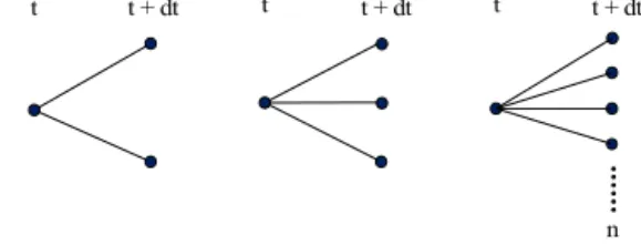
Discretelatticeisastochasticprocess,wherethe stochas-ticvariablecanchangeonlyafterpassingcertaintime-step (steppingtime)andcantake ongivennumberofnew val-ues.Agiventimeperiod(T−t),duringwhichthestochastic processis simulated,isdividedintofinitenumberoftime stepswheredtisthelengthofonediscretetimestep(time interval).Foranydiscretemomentattimethasthe stochas-ticprocessatt+dt(i.e.afterpassingsteppingtime)finite possiblenumberofvalueswhichcantakeon.Accordingto thenumberofvaluesattheendofsteppingtimewework with thefollowing processes:binomial (at t+dt takes on twovalues), trinomial (at t+dt takeson threevalues)or
multinomial(att+dttakesonnvalues),seeFig.1.
Simulation via binomiallattice is thesimplest discrete process.Here,thevalueofunderlying(random)assettakes onattimetthevalueSt;attheendofdiscreteinterval(i.e.
afterpassingsteppingtime)itcaneitherjumpuptoSu
t+dtor
downtoSd
t+dtwithsometransition(risk-neutral)probability.
Iftheprocesscantake ononly positivevalues(typicalfor mostfinancialvariables),weworkwithgeometricversion, whereitholdsforupwardjump,
Su
t+dt=u·St (3.1)
anddownwardjump,
Std+dt=d·St (3.2)
andwhereu(d)areupanddownfactors.Forthesetwo fac-torsit holdsfollowing: u≥1;0<d≤1andd<erfdt<u.The upwardanddownwardfactorsuanddandtransition (risk-neutral)probabilitiesaresetuniquelyinordertodetermine the evolution of underlying asset. Due to the fact that expectedreturnofanyassetisassumedtoberisk-free,the expectedvalueattheendofdiscretestepequalsSt·erf·dt.
Itfollowsthat theexpectedvalue oftheunderlying asset canbewrittenas,
E(St+dt)=St·erf·dt=pu·u·St+(1−pu)·d·St (3.3)
andaftersomerearrangements,
erf·dt=pu·u+(1−pu)·d (3.4) From(3.4)therisk-neutralprobabilityofupwardjumppuis
givenas,
pu= e
rf·dt−d
u−d (3.5)
andfordownwardjumpmustfollows,
pd=(1−pu). (3.6)
The varianceoftheunderlying assetbetweentwo sub-sequent discrete nodes at time t and t+dt is 2dt. And becausethevarianceofrandomvariableisgenerallygiven as2(S)=E(S2)−[E(S)]2,itispossibletowrite
2dt=pu·u2+(1−pu)·d2−[pu·u+(1−pu)·d]2
. (3.7) Substituting for pu from (3.5)—(3.7)and after some
rear-rangementsweget,
2dt=erf·dt·(u+d)−u·d−2·erf·dt. (3.8)
Solving(3.4)and(3.8)andunderthecondition,
u= 1
d, (3.9)
wegetforupwardanddownwardfactorsuanddfollowing formulas,
u=e·√dt, (3.10)
d=e−·√dt. (3.11)
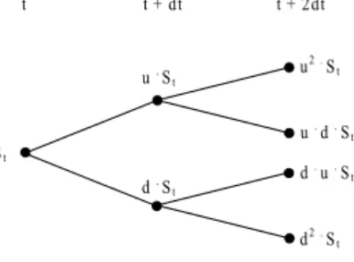
Fig.2showsoneperiodbinomiallatticewithgeometric process. t + dt t u . St d . St St pu pd= 1 -pu
Figure2 Oneperiodbinomiallattice(geometricprocess). t + dt t St + u St -d pu pd= 1 -pu
Figure3 Oneperiodbinomiallattice(arithmeticprocess).
St t + dt t u . St t + 2dt d . St d . u . St d2. S t u2. S t
Figure4 Two-periodrecombiningbinomiallattice(geometric process).
Insituation,thatthesimulatedprocesscantakeonboth positiveandnegativevalues,weworkwitharithmetic ver-sion,whereSu
t+dt=St+uandStd+dt=St−d,seeFig.3.2
Simulationviabinomiallatticewithvolatility
change
Ifweassumetheconstantvolatilityovertheperiod(T−t), theupanddownwardfactorsgivenaccordingto(3.10)and (3.11)areconstantthroughoutthewholelatticemodeland dueto(3.9)itholdsu·d=d·u=1,whichfollowsintheresult thelatticerecombines.This means that thenodes recon-nect,i.e.St+2dt=u·d·StorSt+2dt=d·u·St.Furthermore,the
valueof theunderlying assetin anynode of thebinomial latticecanbeexpressedas,
St+i·dt=uj·di−j·St (3.12)
If(3.10)and(3.11)areunchangedandunderthe assump-tionof constantrisk-freerate,thetransition probabilities betweenanytwosubsequentnodesaccordingto(3.5)and (3.6) are constant, as well. Fig. 4 illustrates two-period recombiningbinomiallatticecanbedepictedasitisshown inFig.4.
When an up move followed by a down move does not reconnectinthesamenodeasadownmovefollowedbyan
2More detailsonderivationcanbefoundinTich´y(2008), Hull (2014),etc.
St t + dt t u . St t + 2dt d . S t d . u . St d2. St u2. S t u . d . S t
Figure5 Two-periodnon-recombiningbinomiallattice (geo-metricprocess).
upmove,i.e.St+2dt =/ u·d·StorSt+2dt =/ d·u·St,thelattice
iscallednon-recombining.Non-recombininglatticeisused foranalysiswhentherearemultiplesourcesofuncertainty orwhenvolatilitychangesover time.Themain difference betweenrecombiningandnon-recombininglatticeis,that thelatticewithnperiodstherecombininghave(n+1)final uniquevalues,whereas non-recombining2n values,which
arenot unique.Fig. 5 shows two-period non-recombining binomiallattice.
Iftheassumptionofconstantvolatilityisrelaxed,it fol-lowsthatupwardanddownwardfactorsaccordingto(3.10) and(3.11)arenotconstantthroughoutthelatticeanymore. The same is true about the transition risk-neutral proba-bilities. In such situations, there are a few ways how to overcomethisissue:(a)foreach periodandvolatility cal-culate corresponding upward and downward factors; the sameis true about thetransition probabilities(b) setthe transitionprobabilitiespu=pd=0.5throughoutthebinomial
latticeandcalculateforeachperiodupwardanddownward factorsaccordingtogivenvolatility,
u=e(rf−2/2)·dt+ √ dt (3.13) d=e(rf−2/2)·dt− √ dt (3.14)
or (c)thesize of upand downmovements and their cor-respondingtransitionprobabilitiesareconstantthroughout the lattice, but the time periods are of unequal length. Whenvolatilityishigh,thetimeperiodsareshort,sothat thestate variablechangesfrequentlybythe standardized amount.Whenvolatilityislower,theperiodsarelongerso thatthe changes inthe state variableare less frequent.3
ThisbinomiallatticeispresentedinFig.6.
Application
—
valuation
American
real
option
valuation
with
changing
volatility
Thispartofthepaperisfocusedontheapplicationof dis-cretebinomiallatticeontherealoptionvaluation(optionto expandaproject).The optionisanAmerican-typeoption, i.e. the project can be expanded at any timeduring the expectedlifespan.Itisassumedthattheunderlyingasset isthecashflowgeneratedbytheproject;theinitialvalue
FCF0=100c.u.,andevolvesaccordingtotheGBM.Company has the option to expand the project at any time during the life span with the costs on expansion IE=80c.u. The
3For more details and mathematical background see Guthrie (2011)orHaahtela(2010).
dt1 dt2 dt3
Figure 6 Three-period recombining binomial lattice with unequallengthoftimesteps.
risk-freerateisrf=8%p.a.andtheannualvolatility=25%.
Theillustrationexampleisstructuredasfollows: I. first,itisassumedthatthevolatilityisconstant, II. next, volatility of cash flow increases as the project
expectedend-lifeisapproaching,
III. intheend,volatilityofcashflowincreasesisassumed again,forproblemsolution,anapproachsuggestedby Guthrie(2011)isemployed.
ProblemsolutionI
Problemsolutionisdecomposedintothefollowingsteps: (a) Calculationofupwardanddownwardfactor.
Substitut-inginto(3.10)and(3.11)wegetu=1.284andd=0.7788. (b) Calculationtherisk-neutralprobabilities.Applying(3.5) and(3.6)wegetfollowing:pu=60.27%andpd=39.73%.
(c) Simulationoftheunderlyingassetviatherecombining andnon-recombininglattice.
(d) Theintrinsicvaluecalculation.Foroptiontoexpandit isdefinedasIVt=max(Vt−IE;0).4
(e) Optionvaluecalculationaccordingto(3.7)byapplying backward-induction approachwith risk-neutral proba-bilities.
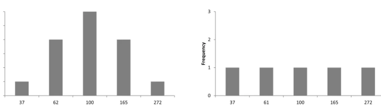
Following Fig.7 shows numerical results; Fig.8 shows thehistogramofendnodevaluesforrecombiningand non-recombining lattice.The results obtainedareidenticalno matterwhichapproachisused(optionvalueequals45c.u.).
ProblemsolutionII
Realoptionvaluationwithchanging volatilityincludes fol-lowingsteps:
(a) Calculationof upwardanddownwardfactors foreach period and volatility according to (3.10) and (3.11). Recall, that the volatility 1 appliesfor thefirst two
4Formoredetailsseeforexample Trigeorgis(1999),Trigeorgis
272 192 192 212 132 138 165 85 85 165 85 97 165 85 85 128 48 55 100 20 20 128 48 66 165 85 85 128 48 55 100 20 20 100 20 34 100 20 20 78 0 11 61 0 0 100 20 45 165 85 85 128 48 55 100 20 20 100 20 34 100 20 20 78 0 11 61 0 0 78 0 21 100 20 20 78 0 11 61 0 0 61 0 6 61 0 0 47 0 0 37 0 0 272 192 192 212 132 138 165 165 85 85 97 85 128 128 48 48 66 55 100 100 100 20 20 20 45 34 20 78 78 0 0 21 11 61 61 0 0 6 0 47 0 0 37 0 0
Non-recombining underlying asset lacce Non-recombining intrinsic value lace Non-recombining valuaon lace
Recombining valuaon lace Recombining intrinsic value lace
Recombining underlying asset latce
Figure7 Realoptionvaluationlattice(recombiningandnon-recombininglattice,constantvolatility).
0 1 2 3 4 5 6 37 62 100 165 272 Fre qu ency
end node values
0 1 2 3 37 61 100 165 272 Fre qu ency
end node values
Figure8 Endnodevaluesofunderlyingassetvaluefornon-recombininglattice(left)andrecombininglattice(right).
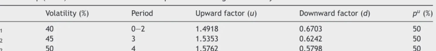
Table1 Up(down)wardfactorsandtransitionprobabilitiesforgivenvolatilitylevel.
Volatility(%) Period Upwardfactor(u) Downwardfactor(d) pu(%)
1 40 0—1and1—2 1.4918 0.6703 50.3
2 45 3 1.5683 0.6376 47.9
575 495 495 349 269 275 212 132 132 223 143 154 234 154 154 142 62 68 86 6 6 149 69 91 259 179 179 157 77 83 95 15 15 100 20 42 105 25 25 64 0 11 39 0 0 100 20 52 259 179 179 157 77 83 95 15 15 100 20 42 105 25 25 64 0 11 39 0 0 67 0 22 116 36 36 70 0 15 43 0 0 45 0 7 47 0 0 29 0 0 17 0 0 575 495 495 349 269 299 223 259 143 179 177 179 149 157 69 77 104 94 100 100 116 20 20 36 60 49 36 67 70 0 0 26 15 45 47 0 0 7 0 29 0 0 17 0 0
Recombining underlying asset lace Recombining intrinsic value lace Recombining valuaon lace Non-recombining underlying asset lace Non-recombining intrinsic value lace Non-recombining valuaon lace
Figure9 Realoptionvaluationlattice(recombiningandnon-recombininglattice,increasingvolatility).
Table2 Up(down)wardfactorsandtransitionprobabilitiesforgivenvolatilitylevel.
Volatility(%) Period Upwardfactor(u) Downwardfactor(d) pu(%)
1 40 0—2 1.4918 0.6703 50
2 45 3 1.5353 0.6242 50
2 50 4 1.5762 0.5798 50
periods, 2 for period three and 3 for period four. ResultsaresummarizedinthefollowingTable1. (b) Simulationoftheunderlyingassetviatherecombining
andnon-recombininglattice. (c) Theintrinsicvaluescalculation.
(d) Optionvaluecalculationaccordingto(3.7)byapplying backward-induction approachwithrisk-neutral proba-bilities.
Fig. 9 shows resulting lattices; Fig. 10 shows the histogram of end node values for recombining and non-recombining lattice. The results obtained are no more identical;thedifferenceis caused primarily bythe larger differencesintheendnodesvalues(andtheirfrequencies)
of the recombining and non-recombining underlying asset lattice.
ProblemsolutionIII
Realoptionvaluationwithchanging volatilityincludes fol-lowingsteps:
(a) Calculation of the upward and downward factors for eachperiodandvolatilityaccordingto(3.13)and(3.14); the transition probability is set to equals 50% for all periods,seeTable2.
0 1 2 3 17 39 43 47 86 95 105 116 212 234 259 575 Fre qu ency
End node values
0 1 2 3 37 61 100 165 272 Fre qu ency
end node values
Figure10 Endnodevaluesfornon-recombininglattice(left)andrecombininglattice(right).
539 459 459 342 262 266 198 118 118 223 143 153 219 139 139 139 59 64 81 1 1 149 69 89 242 162 162 154 74 79 89 9 9 100 20 40 98 18 18 62 0 8 36 0 0 100 20 51 242 162 162 154 74 79 89 9 9 100 20 40 98 18 18 62 0 8 36 0 0 67 0 21 109 29 29 69 0 13 40 0 0 45 0 6 44 0 0 28 0 0 16 0 0
Non-recombining underlying asset lace Non-recombining intrinsic value lace Non-recombining valuaon lace
Figure11 Realoptionvaluationlattice(non-recombininglattice,increasingvolatility).
(b) Simulation of the underlying asset via the non-recombininglattice.Duetothefactthattheu·d =/ 1, itisnotpossibletoconstructtherecombininglattice. (c) Theintrinsicvaluecalculation.
(d) Option valuation according to (3.7) by backward-inductionapproachandapplyingrisk-neutral probabili-ties.
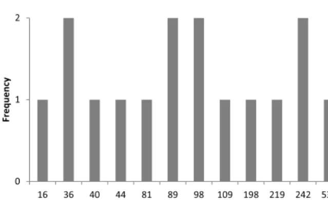
ResultsareagaindepictedinthefollowingFig.11;Fig.12 showsfrequency ofunderlyingassetendnode values.Itis apparentthatthisapproachprovidesthesameresultsasthe oneappliedinProblemsolutionII.5
5Smalldifferenceintheresultsiscausedbythenumberofthe
stepsinvaluationlattice.Forfiveandmorestepstheresultsworld beidentical. 0 1 2 16 36 40 44 81 89 98 109 198 219 242 539 Fr e qu ency
End node values
Figure 12 End node values of underlying asset for non-recombininglattice.
Conclusion
Thispaperfocusesattherealoptionvaluationunder chang-ingvolatility.Changeinthevolatilitystructure(i.e.change
inprojectcashflowsriskiness)isatypicalfeatureformost ofthelong-termproject,wherethepredictionofthecash flowsinthe farfutureis difficult andassociatedwiththe higherrisk.
DuetothefactthatmostrealoptionsareAmerican-style options,therearediscretebinomialmodelsapplied. More-over,otheroptionvaluationmodels(likeB—Smodel)relyon some assumptions(valuation European-style options, con-stantvolatility,riskfreerate)andtheirapplicationmaybe limitedforrealoptionsissuessolutions.
It has been shown that, under changing volatility application of non-recombining lattice with risk-neutral probabilitiesis auseful tool helpingthe analysts to over-come the option-valuation problems associated with the variableparameters.
Therewere twoapproachesemployedtoevaluate real optionwiththevolatilitychange.Theformeroneisbasedon theassumptionthattheentirelatticeisdividedintostages withconstantvolatility;attheendoftheconstantvolatility period,eachresultingpointbecomesstartingpointofanew lattice.Foreachperiod,correspondingupanddownfactors andtransitionprobabilitiesmustbecalculated.Thelatter approachsetsthetransitionprobabilitiesto50%throughout theentirelatticeandadjuststheupanddownwardfactors withrespect tothe volatilityduring given period.Due to thefactthatthecentralityisbroken,onlynon-recombining latticecanbeused.Anyway,forsufficientnumberofsteps bothapproachesprovidethesameresults.
Conflict
of
interest
Theauthordeclaresthatthereisnoconflictofinterest.
Acknowledgements
This paper was supported within Operational Pro-gramme Education for Competitiveness — Project No. CZ.1.07/2.3.00/20.0296andtheProjectNo.GP14-15175P.
References
Black,F.,Scholes,M.,1973.Thepricingofoptionsandcorporate liabilities.J.Polit.Econ.81(3),637—654.
Brach,M.A.,2002.RealOptionsinPractice.Wiley,NewJersey.
Brennan,M.J., Schwartz,E.S.,1985. Evaluatingnaturalresource investments.J.Bus.58(2),135—157.
Brennan, M.J., Trigeorgis, L., 2000. Project Flexibility Agency andCompetition:NewDevelopmentsintheTheoryand Appli-cation of Real Options, first ed. Oxford University Press, London.
Copeland,T.E.,Antikarov,V.,2003.RealOptionsRevisedEdition:A Practitioner’sGuide,seconded.Texere,NewYork.
Cox,J.C.,Ross,S.A.,Rubinstein,M.,1979.Optionpricing:a sim-plifiedapproach.J.Financ.Econ.7(3),229—263.
Damodaran,A.,2006.Damodaran onValuation:SecurityAnalysis forInvestmentandCorporate Finance,seconded.Wiley,New Jersey.
Dixit,A.K.,Pindyck,R.S.,1994.InvestmentunderUncertainty,first ed.PrincetonUniversityPress,NewYork.
Grenadier,S.,2000.GameChoices:TheIntersectionofRealOptions andGameTheory.Riskbooks,London.
Guthrie,G.,2011.Learningoptionsandbinomialtrees.WilmottJ. 3(1),1—23.
Haahtela, T., 2010. Recombining trinomial tree for real option valuation with changing volatility. In: Annual Real Option Conference.
Hoek,J.,Elliot,R.J.,2006.BinomialModelsinFinance.Springer, NewYork.
Hull,J.C.,2014.Options,Futures,andOtherDerivatives,ninthed. PrenticeHall.
Merton,R.,1973.Thetheoryofrationaloptionpricing.BellJ.Econ. Manag.Sci.4(1),141—183.
Mun,J.,2005.RealOptionAnalysis.ToolandTechniquesfor Valu-ingStrategicInvestmentsandDecisions,seconded.Wiley,New Jersey.
Mun, J.,2003. Real OptionsAnalysis Course: BusinessCasesand SoftwareApplications.Wiley,NewJersey.
Smith, J.E., Nau, R.F., 1995. Valuing risky projects: option pricing theory and decision analysis. Manag. Sci. 14, 795—816.
Tich´y,T.,2008.LatticeModels.PricingandHedgingat(In)omplete Markets.VˇSB-TUOstrava.
Trigeorgis,L.,1999. RealOptionsandBusinessStrategy: Applica-tionstoDecisionMaking.Riskbooks,London.
Trigeorgis,L.,Schwartz,E.S.,2001.RealOptionsandInvestments underUncertainty.MITPress,Cambridge.
Trigeorgis, L., Smith, H.T.J., 2004. Strategic Investment: Real OptionsandGames.PrincetonUniversityPress,NewYork.