Changes in the Structure of Wages in the Public and Private Sectors

NBER WORKING PAPERS SERIES

CHANGES

IN THE STRUCTURE OF WAGES

IN THE PUBLIC AND PRIVATE SECTORS

Lawrence F. Katz

Alan

B. Krueger

Working Paper No. 3667

NATIONAL BUREAU OF ECONOMIC RESEARCH

1050 Massachusetts Avenue

Cambridge, MA 02138 March 1991

We thank Kevin M. Murphy for providing us with data from the

March Current Population Surveys and for helpful discussions. We

are grateful to Ana Maria Lusardi and Kainan Tang for expert

research assistance, and to Phillip Schneider and Andrew Klugh

for providing us with data from the Central Personnel Data File

of the U.S. Office of Personnel Management. We have benefitted

from the coments of Claudia Goldin, Ron Johnson, and seminar

participants at Harvard, Princeton, UCLA, UCSD, MIT, and the

University of Chicago. Financial support from National Science

Foundation Grant SES9010759, the Princeton Industrial Relations

Section, and an NBER Olin Fellowship in Economics is gratefully

acknowledged. This paper is part of NBER's research program in

Labor Studies. Any opinions expressed are those of the authors

and not those of the National Bureau of Economic Research.

NBER Working Paper #3667

March 1991

CHANGES IN THE

STRUCTURE

OF WAGES IN THE

PUBLiC AND PRIVATE SECTORS

ABSTRACT

The wage structure in the U.S. public sector responded

sluggishly to substantial changes in private sector wages during

the 1970s and 1980s. Despite a large expansion in the

college/high school wage differential during the 1980s in the

private sector, the public sector college wage premium remained

fairly stable. Although wage differentials by skill, in the

public

sector

were fairly unresponsive to changes in the private

sector, overall pay levels for state and local government workers

were quite sensitive to local labor market conditions. But

federal government regional pay levels appear unaffected by local

economic conditions. Several possible explanations are

considered to account for the rigidity of the government internal

wage structure, including employer size, unionization, and

nonprofit status. None of these factors adequately explains the

pay rigidity we observe in the government.

Lawience F. Katz

Alan B. Krueger

Department of Economics

Industrial Relations

Littauer Center Section

Harvard University

Firestone Library

Cambridge, MA 02138

Princeton University

I. Introduction

Recent research has documented sharp changes in the structure of wages

and substantial increases in wage dispersion in the United States over the

last twenty years.1 The college wage premium, after narrowing in the 1970s,

increased markedly in the l9BOs. Wage differentials by experience expanded

from the early 1970s to the late l980s, and residual wage inequality

(earnings dispersion within detailed education-experience groups) increased

for both men and women in the l970s and l980s. Typically, however, this

literature has not determined whether these wide-ranging changes have been

confined to the private sector or whether they are shared by public and

private employees alike, We document in this paper that overall wage

structure changes in the l970s and 1980s have been driven by events in the

private sector. These private sector changes provide a natural benchmark for

examining how public sector wages respond to movements in labor market

conditions.

We examine three questions concerning public sector pay flexibility in

the federal government and in state and local governments. The first is the

extent to which public sector wage policies respond to market changes in

skill differentials. The second is the extent to which government pay levels

respond to differences in local labor market conditions. In particular, we

explore how wages in different branches of government are affected by changes

in private sector skill premia and by local private sector wage levels and

unemployment rates. Finally, we examine the implications of government pay

polices for the ability of government agencies to meet their personnel

1Srudies examining recent changes in the U.S. wage structure include Blackburn, Bloom, and Freeman (1990), Bluestone (1990), Bound and Johnson (1989), Davis and Haltiwanger (1991), Juhn, Murphy, and Pierce (1989), Karoly (1990), Katz and Murphy (1990), Katz and Revenga (1989), and Murphy and Welch

requirements.

Answers to these questions are necessary to understand and evaluate the public sector personnel management systems, which directly affect the nearly one-fifth of employees in the United States who are employed by some branch

of government.2 Furthermore, government pay practices can have a substantial

impact on the operation of private sector labor markets in which the government is a major employer, such as the markets for health service

workers, scientists, teachers, and engineers, Smith (1977) has argued that

there are many reasons to suspect that ordinary market forces will not lead the government to optimally alter its personnel and compensation practices.

Many observers have already voiced concern that the government (especially

the federal government) will be increasingly unable to recruit highly skilled

employees -- such as scientists, engineers, and judges --

unless

its wage

structure responds to changes in the private sector wages (e.g. Campbell and Dix, 1990; National Commission on the Public Service, 1989).

In section II, we analyze a variety of micro-data sets from the Current Population Survey (CPS) and other sources to examine whether the government wage structure has, in fact, been rigid in the face of changes in the private

sector wage structure. We compare and contrast changes in wages by

education, experience, and gender in the public and private sectors during

the l970s and l980s. Despite the large expansion in private sector wage

differentials by skill level in the 1980s, we find that skill differentials

remained fairly stable in the public sector in the l9SOs. In particular, the

pay of workers at the upper part of the federal pay scale has fallen

2See Ehrenberg and Schwarz (1986) for a discussion of U.S. public sector labor market institutions and a critical survey of research on public sector labor markets.

3

substantially relative to "comparable" private sector workers, and the wages of less-educated employees of state and local governments have increased

greatly relative less-educated private sector workers. The sharp increase

during the 1980s in the college/high school wage differential of the l980s is almost entirely a private sector phenomenon.

In section III, we examine variation in pay across states in the private

and public sectors. Ceographic variation in pay at a moment in time is quite

similar for workers employed in the private sector and for those employed by

state and local governments. Changes in local labor market conditions (as

proxied by state unemployment rates) seem to have a similar effect on private

and on state and local government wage levels. We find that state and local

governments alter overall wage levels in response to economic conditions that

are likely to affect government budgets and the tax base. Their response is

similar to how private sector employers, operating in industries with

localized product markets, respond to changes in local economies. In

contrast to the responsiveness of their overall wage levels, state and local governments sluggishly adjust relative wages by skill category to shifts in

the private sector wage structure. Regional pay variation appears quite

different in the federal government. Here pay does not closely mimic local

wage structures and does not seem to respond to changes in local labor market

conditions. We present some evideoce that this rigidity owes to a single

national wage schedule for most federal government employees. In section IV, we explore several possible explanations for the

stability of public sector skill differentials in the l980s. We first

examine the roles played by employer size, nonprofit status, and

4

for wage structure rigidity in the government. Educational wage

differentials expanded sharply in the 1980s in large, private-sector firas

and in private sector industries dosinated by nonprofit firms. Furtheraore,

we find that public sector skill differentials increased auch less than those in the private sector even in the ten states with the lowest public sector

unionization rates. Finally, we briefly discuss other institutional

explanations for the relative rigidity of government pay structure. In section V, we empirically examine how increases in wage compression in the public sector relative to the private sector in the l980s has affected

public sector personnel outcomes. We analyze how wage rigidity in the

federal government has affected its ability to recruit and retain employees

of different skill levels. Job queues have indeed expanded for blue-collar

jobs and contracted for white-collar jobs in the federal government in the

l9g05. Furthermore, the federal government also seems to be having

difficulty in retaining college graduates whose skills are valued highly in the private sector.

II. Changes in Public and Private Wsge Structures Over Time

We use several individual-level data sets to compare wage structure changes in the U.S. public and private sectors over the last twenty years. Before turning to this micro analysis, we first examine longer-term trends in

the relative pay of public sector workers using aggregate data from the National Income and Product Accounts (NIPA) for the entire postwar period.

Figure 1 presents NIPA data on the ratio of total compensation, and of

0 ri

4-, (t, >..

a

a) 4-, (U

>

C-

a

U

'-4

.0

a

I I I I I I — 1 ——

48

50

55

60

65

70

75

80

85

89

Year

Figure

1:

Public/Private

Pay

Patios,

1948—89,

NIPA

Data

5TT3

o

Wages,

Federal

Civilian

•

Total

Cornp,

Fed

Civilian

+

Wages,

State

6

Local

c

Total

Camp,

State

&

Local

1.45

-

1.4

-

1.35

-

1.3

-

1.25

-

1.2

-

1.15

-

1.1

—

1.05

-

.95

-

.9

-

workers for 1948 to l989. Average pay has remained much higher in the

federal government than in the private sector or in state and local

governments, and trends in relative public sector pay by branch of government

were fairly similar over much of the period. From the mid l950s to the early

l970s, public sector pay rose relative to the private sector. The period

corresponds to a growth spurt in employment demand in the public sector as public sector employment steadily expanded from 13.1 percent of civilian employment (measured in full-time equivalents) in 1955 to 17.9 percent in

1975. Relative public sector pay declined in the late l970s as public sector

employment growth stagnated and the share of employment in the public sector

started a steady decline that lasted through the 1980s. Despite declining

relative employment, the relative pay of employees in state and local

governments increased in the l98Ds. The picture is less clear for the pay of

federal civilian employees relative to private sector workers. If one

examines wages and salaries alone, federal relative pay sharply declined in

the l980s. If, instead, one includes nonwage compensation, federal relative

total compensation increased because nonwage compensation (particularly

pension contributions) rose sharply relative to the private sector. As we

show below, the aggregate trends in the 1980s hide substantial differences in movements in relative public sector pay by education and skill group.

3The figure plots public/private sector ratios of pay per full-time

equivalent employee. Total compensation includes wages and salaries,

employer contributions to social insurance, and employer contributions to

private pension and welfare funds. The Federal Civilian sector includes

civilian employees of the Federal government and of government enterprises. The data used in Figure 1 are fros the U.S. Departsenr of Cossnerce, Bureau of Economic Analysis, National Income and Froducts Accounts.

6

A. gasic Relative Wage Changes. 1967-87

Our comparative analysis of wage structure changes begins with an

examination of movements in the college/high school wage differential by

sector. Many occupations in the government have few close private sector

analogues, if any. Thus movements in education differentials by sector

provide the most meaningful measure of movements in skill differentials in

the public and private sectors.

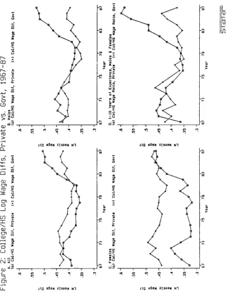
Panel A of Figure 2 presents a plot of the log weekly earnings

differential between college and high school educated workers in the

government and private sectors from 1967 to 1987. The earnings differentials

have been adjusted for changes in the age and gender composition of the

government and private sector labor forces. The plot is based on data from

the March CI'S Annual Demographic Files from 1968 to 1988. Relative earnings

of college graduates declined in both the public and private sectors in the

1970s. In contrast, a sharp increase in the average earnings of college

educated workers relative to high school educated workers occurred in the

'We define high school graduates as individuals with exactly 12 years of

schooling and college graduates as those with 16 or more years of schooling.

To generate Figure 1, we sorted the individual-level data on high school and

college graduates from the March CI'S Surveys into 64 cells based on sex, two

education categories (12 and 16 or more years of schooling), eight potential experience brackets (five-year intervals), and two sectors (private and government). The mean log weekly wages for full-time workers in each of these cells was computed. College/high school log wage differentials for each of our 32 sex-experience-sector categories are then given by the difference in these cell means for the college and high school workers in the category. The numbers plotted in Figure 1 are fixed-weighted averages of the college/high school log wage differentials for the relevant categories in each graph. The fixed-weights are the average share of the sex-experience group in total employment in all sectors over the entire 1967-87 period. The

March CI'S samples provide information on the earnings and weeks worked in the

calendar year preceding the March survey. The sample selection rules used in

the creation of the March CI'S extract are described in detail in Juhn, Murphy, and Pierce (1989) and Katz and Murphy (1990).

Figure

2:

Coilege/HS

Log

wage

Diffs,

Private

vs.

Govt,

1967—87

A. 0)) 8. Holes to) Cot/OS Wage Dl), PrIvate (0) Cot/HG 008e DII. Govt lot Cot/HG Wage CII, PrIvate to) Col/HS Wage DII. Govt .6 _.55 .6 _.55 5 ₄₅ .4 .3 .6 _.55

0

0. .45 .4 .35 .3 67 1•t 7•g 83 87 Year c. Females to) Cot/OS Wage Ott, Prlvatl (0) Cot/OS Wage CU, Govt .3 67 71 75 79 83 81 Year 0. 1—50 Years 01 EapertenCe, 4481ev 8 Feeales Cal Cal/OS Waga RatIo, Private tat Cal/OS Wage ROUO, Govt .6 _.55 .5 _.45 .4 _.35 67 71 75

7

03 07 Yea, .3 67 71 75 79 83 07

5TaTa"

private sector in the 1980s, with the college/high school wage differential

for males and females combined rising from by 15 log points from 0.36 in 1979

to 0.51 in 1987. But the gap in earnings between college educated and high

school educated workers in the government sector increased by only 3 log

points from 0.39 in 1979 to 0.42 in 1987. This rather moderate increase

reflected a combination of a constant differential in the federal government

and an increase of about 4 log points in the state and local government

sector. Panels B and C of the figure illustrate that from 1979 to 1987 the

college wage premium expanded by much less in the public sector than in the

private sector for both men and women. Finally, Panel 0 shows that this

divergence in relative wage patterns in the private and public sectors in the

l980s was most extreme for young workers.

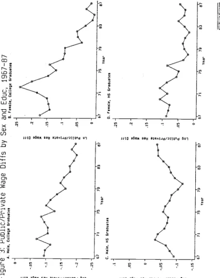
The divergence in educational differentials between the public and

private sectors in the l980s could have occurred because of a relative

decline in public sector pay for highly educated workers, a relative increase

in the public sector earnings of high school graduates, or a combination of

the two. Figure 3 plots trends in public/private wage differentials by level

of education. More precisely, the figure presents the difference between the

actual average public sector wage and the predicted average wage of public

sector workers if they were employed in the private sector (based on a

private sector wage regression) for each group of public sector workers. We

estimated a log weekly wage regression for private sector workers in each

year by gender and education group (high school and college) using the March

CPS samples for calendar years 1967-87. The regressions were of the form:

.25 0 Year

STaTa,'

Figure

3:

Public/Private

Wage

Diffs

by

Sex

and

Educ,

1967—87

A. Male, College Graduale B. Feaale, College Gradoates .25 —.05 -.1 -.2 -.25 &7

7

7

7

8') &1 Year C. Male, tIE Or000atea .1

6'

7'l

7

7

&3 87 Year 0. Feacle, HO Eradoatea .2 .15 .1 .05 Year

8

where W is the weekly wage rate, X is a vector of explanatory variables

including a quartic in experience (and dummies for individual years of

schooling beyond 16 years for college graduates), is the vector of

private sector coefficients for group j in year t. The public/private wage

differential for group j in year t is given by the average value for public

sector workers in group j of lnJ

-X1fi.

During the period of increase in the overall public/private sector pay

ratio from the late 1960s to the early 1970s, Figure 3 indicates that

public/private differentials increased moderately for all groups.

Furthermore, all groups shared in the decline of public sector relative pay

of the late l970s. Previous work has documented the decline in the public

sector wage premium from the aid-l970s to the early 1980s (Freeman, 1987;

Moulton, 1990), but it has not adequately examined how different educational

groups shared in this decline. In the 1980s, the public/private wage

differential continued to drop for college graduates, while the relative

position of male high school graduates in the public sector improved

substantially. The decline of relative public sector wages for college

graduates generated a large negative differential for males and eliminated

the historically large positive differential for females. At the federal

level, the wage premium for male college graduates also withers away,

underscoring recent concerns that the federal government is increasingly

unable to attract skilled professionals,

8. Detailed Analysis of Changes in Relative Wages. 1973-88

years of the Full Year Outgoing Rotation Group (ORG) files of the CE'S and the

May CPS 1973-1975 to estimate a series of wage regressions.5 These data sets

indicate in which branch of government a worker is currently employed, and contain usual weekly earnings and usual weekly hours on the current job.6

We divided the sample into eight subsamples by sex, experience (0-19

and 20+ years), and education (12 and 16 or more years of schooling) for both

the private and public sectors. Wage equations of the form

lnW —a. +b X. +e.

lit it it tjt ijt

were

estimated for each of the subsamples, where W is the hourly wage rate, X

is a vector of personal characteristics (education, two race dummies, an

5Each May CE'S from 1973 to 1978 contains about one-third as many

observations as the Full Year Outgoing Rotation Group Files, available since 1979. We pooled the May 1973 and 1975 CPS's together to provide a larger sample of data. The May 1974 tape that we were able to access lacked

information on level of government and wss not used.

6Wages each year were converted to 1988 dollars using the personal

consumption expenditures implicit price deflator (PCE). Workers who failed

to report usual weekly earnings (those with allocated wages) were dropped from the sample. One limitation of the CE'S is that edited usual weekly

earnings variable is topcoded at $999 in current dollars. The unedited usual weekly earnings variable, however, is top coded at $1,999, but this field is only available for the ORG sample after 1985. The following crude procedure was used to overcome the censuring problem. First, we calculated the mean log hourly wage rate of those in 1988 who had top-coded edited usual weekly earnings using the 1988 unedited weekly earnings variable. This figure was

then assigned to each individual in the 1988 CE'S whose edited weekly wage was

top coded. If few people are censored by the $1,999 earnings limit on the unedited field, this procedure will lead the expected value of the error in the regressions to be approximately zero. We used a similar procedure to deal with top coding in the 1979 and 1983 ORG samples. We converted the top coded amount in 1979 (1983) into 1988 dollars and used the distribution of the unedited weekly earnings variable from 1988 to calculate the mean log hourly wage rate in 1988 dollars of those ropcoded in 1979 (1983) and

assigned this figure to earh individual topcoded in 1979 (1983) .

Since

less

than 0.2 percent of workers are topcoded prior to the late l97Os, we ignored

10

experience spline, SMSA, and part-time status), i is a subscript for

individuals, j indicates the individual's sector of eaployment (public or

private), and t

is

the year.7 The results are also given separately for

federal government workers and for state and local government workers.

The predicted wage rate each year for the four sectors (private,

public, federal, state and local) was calculated by the

gender-experience-education groups for a hypothetical worker with constant characteristics

--white,

full-time, selected experience levels, and residence in a metropolitan

area. That is, we formed the predicted wage

K [ln W, X° ] —

+

bX°.

where X° is the characteristics of the hypothetical worker. This approach

standardizes the wages comparisons for differences in these characteristics

between sectors at a point in time, and for compositional changes within

sectors over time.

Table 1 reports these "regression-adjusted" means for men and women at

two levels of experience in the 1970s and 1980s. Because changes in the wage

structure are likely to occur more rapidly and most sharply for newly hired

workers on the "active labor market" (e.g., Freeman, 1977), our discussion

focuses primarily on the group of workers with little experience. As Smith

(1977), Krueger (1988a), and others have noted, federal workers earn more

than private sector workers, while state and local government workers (who

7The experience variable is defined as age minus education minus six.

Furthermore, we specified the experience effect as a apline function with two terms for each of our subsamples, with a break point in the spline function occurring at 10 years for the 0-20 year experience group and 30 years for the

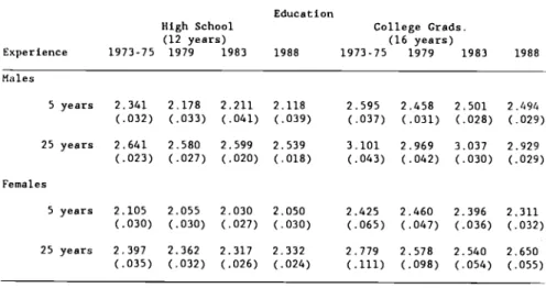
Table 1: Estimated Mean Log Real Hourly Wage Rates

by Education, Experience, Gender and Sector

Class of Worker: Private Sector

Education

High School College Grads.

(12 years) (16 years) Experience 1973-75 1979 1983 1988 1973-75 1979 1983 1988 Males 5 years 2.197 2.182 2.017 1.967 2.505 2.472 2.414 (.006) (.006) (.005) (.005) (.011) (.010) (.008) 2.443 (.008) 25 years 2.565 2.573 2.518 2.467 2.975 2.940 2.919 (.008) (.008) (.007) (.007) (.021) (.020) (.016) 2.908 (.013) Females 5 years 1.915 1.905 1.839 1.800 2.178 2.212 2.233 (.006) (.005) (.005) (.005) (.020) (.013) (.009) 2.290 (.008) 25 years 2.067 2.080 2.053 2.053 2.288 2.270 2.265 (.009) (.008) (.006) (.006) (.041) (.032) (.024) 2.378 (.019)

Class of Worker: All Government

Education

High School College Grads.

(12 years) (16 years) Experience 1973-75 1979 1983 1988 1973-75 1979 1983 1988 Males 5 years 2.212 2.081 2.027 2.029 2.463 2.349 2.306 (.021) (.019) (.018) (.018) (.016) (.016) (.014) 2.310 (.015) 25 years 2.563 2.523 2.490 2.490 2.902 2.828 2.810 (.017) (.017) (.014) (.013) (.027) (.024) (.020) 2.795 (.017) Females 5 years 1.988 1.958 1.935 1.943 2.323 2.242 2.221 (.017) (.015) (.014) (.016) (.014) (.014) (.012) 2.258 (.011) 25 years 2.135 2.113 2.093 2.157 2.518 2.411 2.422 (.018) (.016) (.013) (.012) (.025) (.025) (.019) 2.468 (.016)

Table 1: continued

Class of Worker: Federal Government

Experience High School (12 years) 1973-75 1979 1983 Education 1988 College Grads. (16 years) 1973-75 1979 1983 1988 Males 5 years 2.341 2.178 2.211 (.032) (.033) (.041) 2.118 (.039) 2.595 2.458 2.501 (.037) (.031) (.028) 2.494 (.029) 25 years 2.641 2.580 2.599 (.023) (.027) (.020) 2.539 (.018) 3.101 2.969 3.037 (.043) (.042) (.030) 2.929 (.029) Females 5 years 2.105 2.055 2.030 (.030) (.030) (.027) 2.050 (.030) 2.425 2.460 2.396 (.065) (.047) (.036) 2.311 (.032) 25 years 2.397 2.362 2.317 (.035) (.032) (.026) 2.332 (.024) 2.779 2.578 2.560 (.111) (.098) (.054) 2.650 (.055)

Class of Worker: State and Local Government

Experience High School (12 years) 1973-75 1979 1983 Education 1988 College Grads. (16 years) 1973-75 1979 1983 1988 Males 5 years 2.170 2.054 1.999 (.025) (.022) (.019) 2.006 (.021) 2.398 2.289 2.233 (.018) (.018) (.016) 2.245 (.017) 25 years 2.497 2.495 2.429 (.023) (.021) (.017) 2.455 (.017) 2.739 2.699 2.646 (.032) (.030) (.025) 2.714 (.022) Females 5 years 1.928 1.921 1.904 (.021) (.016) (.016) 1.897 (.018) 2.307 2.215 2.193 (.014) (.014) (.012) 2.248 (.012) 25 years 2.029 2.029 2.031 (.020) (.016) (.013) 2.102 (.013) 2.485 2.391 2.403 (.026) (.026) (.020) 2.449 (.017)

Table 1: continued

Note: Each eatimate is from a separate cross-section regression for an education-experience-gender-sector group of log real hourly earnings on a linear spline of years of experience with a break every ten years, 2 race dummy variables, and dummy variables for metropolitan area and part-time status. The education classes

used are exactly 12 and 16 or more years of schooling; the experience classes are

0-19 and 20 or more years of potential experience. The regressions for college graduates include dummy variables for individual years of schooling. The

estimates for each group are the predicted values of the log hourly earnings

regression for that group evaluated at the indicated schooling and experience

levels and for a full-time, white employee living in a metropolitan area.

Sources: The data used are from the May 1973 and 1975 CPSs and the Full-Year 1979,

1983, and 1988 CPSs (Outgoing Rotation Groups). The samples used include wage and

salary workers who do not have imputed (allocated) earnings. Earnings are deflated

by the personal consumption expenditures implicit price deflator for GNP and are

in 1988 dollars.

I

11

dominate

the all government

category) earn less than observationally

equivalent private sector workers. The federal pay differential is

especially large for women.

The table also reinforces the findings of Figures 1 and 3 by

indicating that government workers' earnings (even for workers with a fixed set of characteristics) decreased substantially relative to private sector

workers between the mid and late 1970s. For example, from 1973 to 1979 real

government wages fell by 12% for high school educated men with five years of

experience, but fell by only 1.5% for similar private sector men. Inflation

eroded government workers' pay far more than it eroded private sector

workers' pay in the 1970s. In fact, time series analysis using NIPA data

indicates a general tendency for public/private sector pay ratios to decline during periods of rapid price deflation (Freeman, 1987).

In contrast to the l970s, the figures for the 1980s show a huge decrease in the real wage rate of less-educated workers in the private sector, while less-educated workers in the government experienced a much smaller decline in

real wages. For young, male high school graduates the real average wage rate

fell by more than 20% in the private sector in the decade between 1979 and 1988, while the real wage of similar government workers fell by only 5% over the same time period.

Evidence on changes in nonwage compensation suggests that the relative

gain in total compensation made by less-educated government workers in the

1980s was even greater than indicated by the wage changes in Table 1. Data from the NIPA indicate that from 1979 to 1988 the nonwage share of total

compensation increased from 15.5 to 21.8 percent in the federal government

12

share actually fell slightly from 15.4 ro 15.1 percent over the same period

in rhe privare sector. The relative decline in nonwage benefits in the

private secror is likely to have been most important for less-educated

workers. For example, tabulations from the May 1979 and May 1988 CPS Pension

Supplements indicate that the share of workers with 12 years of schooling

covered by employer health insurance declined from 46 to 42 percent in the

private sector end increased from 56 to 61 percent in the public sector from

1979 to 1988.8 No similar relative private sector decline in health

insurance coverage for college-educated workers is apparent: the fraction of

employed college graduates covered by health insurance increased from 75 to

78 percent in the private sector and from 80 to 84 percent in the public

sector over this period. Thus the consideration of nonwage benefits is

likely to have expanded public sector compensation gains for less-educated

workers in the 1980s and may not have greatly affected public/private sector

relative compensation changes for more-educated workers.

The wage patterns shovn in Table 1 imply that the college/high school

log wage differential for males with 5 years of experience increased from

0.29 in 1979 to 0.48 in 1988 in the private sector. In the public sector

over the same period, the wage differential remained fairly stable increasing

by only 0.01, from 0.27 to 0.28. Similarly, experience differentials for

high-school workers increased by much more in the 1980s in the private sector

than in the government.

Women who were college graduates in the private sector experienced

substantial gains in earnings in the 1980s, while earnings remained

relatively constant for college educated women in the public sector. As a

8These tabulations were provided to the authors by Jonathan Gruber.

13

result of the latter trend, young college educated women, who earned 15% more b

in

rhe government than in the private sector in the early 1970s, now earn

slightly less in the government than in the private sector.

In general, the trends detailed in this section suggest that the government sector has been fairly unresponsive to the major swings in the

wage structure that occurred in the private sector in the 1980s. As a

consequence, the government wage structure has become even more compressed

relative to the private sector. The adjustment has been most sluggish for

recent labor market entrants with advanced degrees.

Another important trend worth noting is that in the early 1970s more than 65% of college educated female workers were employed by some branch of

government, but by 1987 only 42% of all college educated women (and less than

30% of those with 1 to 5 years of potential experience) were employed by the

government. Although the government remains an important source of

employment for well-educated women, it clearly has decreased in importance. Furthermore, female college and high school graduates gained approximately 8-14 percent on males with similar levels of education and experience in the

private sector in the l980s; the analogous groups gained just 4 to 8 percent

in the public sector. Thus, despite the comparable worth movement in the

public sector in the 1980s, private sector employment and earnings growth for

women have been largely responsible for the substantial narrowing of the gender gap in earnings since the late l970s.

C. Wame Differentials in the Federal Government. 1976-88

14

difficult to draw precise conclusions about changes in educational wage

I

differentials in the federal government, we use a large extract of micro-data

from the Central Personnel Data File (CPDF) of the U.S. Office of Personnel

Management (DPM) to analyze changes in the college wage premium in the

federal government from 1976 to 1988. This extract contains over 1.4 million

observations and includes information on workers' annual salary, tenure, age, occupation, and other characteristics for a 10 percent random sample of full-rime, permanent General Schedule-equivalent and blue-collar workers in the federal government for even-numbered years from 1976 to 1988.

We used the CPDF to estimate cross-section regressions by gender and

year for samples of workers with exactly 12 and exactly 16 years of

schooling. The dependent variable is the log annualized salary, and the

independent variables are a quartic in potential experience (age -

years

of

schooling -

6),

three race dummies, seven interaction terms between a college

graduate dummy variable and dummy variables for experience brackets (0-5,

6-10, 11-15, 16-20, 21-25, 26-30, and 31+ years), and an interaction term

between the black dummy and the college graduate dummy. The estimated

college/high school wage differentials by gender and experience from these

regressions for 1976, 1980, 1984, and 1988 are presented in Table 2.

Table 2 indicates that the college wage premium expanded only moderately

in the federal government in the l98Ds. In contrast to the greater than 20

log point increase in the college/high school differential for young workers

in the private sector, the college wage premium increased by only about S log

points for those with less than 5 years of experience in the federal

government. Increases for more experienced workers were also much more

moderate than those for the private sector.

Table 2: College/High School Log Wage Differentials for Full-Time Workers

in the U.S. Federal Covernmenr 1976-1988

Experience Group 1976 1980 1984 1988 Males 0-5 years 0.291 (0.008) 0.280 (0.010) 0.287 (0.010) 0.327 (0.009) 6-10 years 0.322 (0.005) 0.336 (0.006) 0.299 (0.006) 0.328 (0.007) 16-20 years 0.383 (0.006) 0.368 (0.006) 0.377 (0.005) 0.347 (0.005) 26-30 years 0.368 (0.006) 0.334 (0.007) 0.362 (0.006) 0.373 (0.006) Females 0-5 years 0.343 (0.006) 0.341 (0.007) 0.370 (0.008) 0.399 (0.008) 6-10 years 0.395 (0.008) 0.388 (0.007) 0.397 (0.009) 0.405 (0.007) 16-20 years 0.317 (0.014) 0.358 (0.012) 0.365 (0.009) 0.371 (0.007) 26-30 years 0.295 (0.013) 0.242 (0.013) 0.243 (0.012) 0.283 (0.011)

Note: The reported estimates are from cross-section regressions of log annualized

salary on a quartic in experience (age -

years

of schooling -

6),

3 race dummies,

7 interaction terms between a college graduate dummy variable and dummy variables for experience brackets (0-5, 6-10, 11-15, 16-20, 21-25, 26-30, and 31+ years), and an interaction term between the black dummy and the college graduate dummy.

Separate regressions were run for each of the indicated years by gender for samples containing Federal workers with exactly 12 or exactly 16 years of

schooling. Each reported estimate is the coefficient on the interaction term

between college graduate status and the indicated experience bracket dummy

variable. The numbers in parentheses are standard errors. Sample sizes for males

(females) are 62,091 (40,511) in 1976; 59,718 (44.171) in 1980; 65.189 (47,829) in 1984; and 64,936 (52,875) in 1988.

Source: The data are from the U.S. Office of Personnel Management's Central

Personnel Data File (CPDF) and cover full-time, permanent CS-and-equivalent and blue collar federal employment.

15

D. Changes in Public/Private Sector Wage Differentials by Percentile

Civen the compression in government pay relative to the private sector

nored above, there has been a great deal of concern that the government is

unable to recruit qualified workers at the high-end of the skill

distribution. This concern is especially strong in the federal government,

as demonstrated by the formation of the National Commission on the Public

Service to study this issue. Consequently, we next contrast trends in pay at

the upper and lower ends of the earnings distribution in the government and

the private sector.

Figure 4 plots the federal/private log hourly wage differential by

percentile for full-time college and high school graduates by sex for 1979

and 198g. These plots compare the log hourly earnings of federal and private

sector employees who hold the same relative position within their respective

earnings distributions. The plots use wage residuals to control for

differences in the wage distributions arising from differences in the age, location, and race coapcsitions of the workforces in each sector.

Specifically, we estimate regressions of log hourly earnings on a quartic in

years of potential experience, eight region dummy variables, two race dummy

variables, and a metropolitan area dummy variable. Separate regressions are

estimated for full-time, private-sector workers in four education-sex groups

in 1979 and in l98g. Wage residuals for each individual in the federal and

9The two education groups examined are college graduates and high school graduates. The earnings regressions for college graduates include two dummy variables for 17 and for 18 or more years of schooling. Since we are interested in looking at the entire wage distribution and since a substantial fraction of workers in some groups in 1988 have edited usual weekly earnings

that are top coded at $999 (e.g., over 20 percent of male college graduates ₄

are

top coded in 1988) , we use the unedited usual weekly earnings variable

—2 -.25 —3 lb 2b 3o ib sb 60 7b so gb ido Percent lie C. Males, 12 Years of Scnoolln 0 1 1979 (5)

l8B

lb 20 30 40 50 60

7

eo gb

,d

Percentile 0. Females, 12 Yea,! of 00080lin 1 1979 181 198

-C-

III

liii,,

10 20 30 40 50 60 70 00 90 100 Percentile

Figure

4:

Federal

Govt/Private

(Residual)

Wage

Diffs

by

Percentile

A. Males, 16 or more Years of Schooling B. Females, 16 or more Years of Schooling 1 1 1979 (5) 1988 1 I 1979 1,1 1909 .35 .3 .25 .2 .15 .05 0 -.05 -.15 .4 .35 .25 .15 .05 .35 .3 .25 .2 .15 .1 .05 0

ib

20 30 40 50 6b

ib

80 gb 100 Percentile

5TaTa''

16

private sectors are given by the difference between actual and predicted log

hourly earnings. Predicted earnings for an individual are calculated using

the individuals observed characteristics and the estimated coefficients from

the private sector earnines function for that individuals education-sex

group.

Figure 4 illustrates pay compression in the federal government relative

to the private sector. It is clear that the earnings advantage of federal

workers is much greater at the bottom part than at the top part of the

earnings distribution in each group. Panel A shows that for msles with

college degrees the substantial earnings premium of federal workers in the

bottom fifteen percent of the distribution remained steady from 1979 to 1988,

but the relative earnings of federal workers declined at an increasing rate

as one moves up the earnings distribution. From 1979 to 1988, the earnings

of college-educated males in the top quintile of the federal government

earnings distribution fell by approximately 10 percent relative to private

sector workers in comparable positions in the earnings distribution. In

fact, the log (residual) wage differential between the 90th percentile and

10th percentile workers increased by 0.07 in the private sector and declined

by 0.03 in the federal government for male college graduates from 1979 to

1988. Panel B shows a similar pattern for college-educated females.

Figure 5 uses the same approach as Figure 4 to display wage

differentials by percentile between state and local government and private

for 1988 in our analysis of wage changes by percentile. The wages of individuals with usual weekly earnings top coded at $999 in 1979 and at $1999

in 1988 are adjusted by multiplying the wages of such workers by 1.40.

Since changes at the very top end of the (residual) earnings distribution appear to be quite sensitive to the treatment of top coded wages, we truncate

the plots presented in Figures 4 and 5 at the 95th percentile.

—

—

.—

-.

e

—-—

-

———

———

-—

—-

---—-———-

p .3 .25 .2 10 28 3b 40 50 60 7b eb gb ado Percentile 0. resale,, 12 Years at ScYeYlin I 1979 (41 198 20 ab

o

so so 7b ob ab ado Percentile .25 .2 Is .1 .05 0 -.05 —.1

Figure

5:

State

C

Local/Private

(Residual)

Wage

Outs

by

Percentile

A. Hales, (8 or mere Veers 5! SchoolIng 8. resale,, 16 or sore Years of Schoa11e 1 a 1979 C.) 1986 I 1 1979 +1 1909 .3 S -.15 .3 .25 'Is .1 .05 -.05 —'I -'IS to 20 30 ib so so ob eb 9o ida Percentile C. Hales, 12 Years al Scoosling I I 1979 Ia) 1008 3 .15

'I

.05 —.05 —'I —.15 ab 20 3b 40 sb sb 7b Wo ab ido Percentile

sTaTa"

17

sector wotkers for 1979 and 1988.10 Panel A of Figure 5 shows some small

gains at the bottom end of the distribution and small losses at the top end

for male college graduates in state and local governments relative to the

private sector. Panel 8 of Figure 5 indicates a significant decline in wages

relative to the private sector for female college graduates in the top half

of the earnings distribution in the state and local sector.

In contrast, panels C and D of Figures 4 and 5 show a quite different

pattern for high school graduates. For high school educated workers the

premium for working in the federal government increased throughout most of

the earnings distribution for both male end females in the l980s, but

decreased at the upper end for males. The earnings of high school graduates

in state end local government increased relative to private sector workers

throughout the distribution.

Taken together, Figures 4 end S tell strikingly different stories for

low-paid end high-paid workers in the government relative to the private

sector. Over the lest decade, less-educated workers fared extremely well in

the government relative to the private sector, while highly-educated federal

workers lost ground. Upper-tail federal workers now earn substantielly less

then upper-teil private sector workers. In the state end locel government

sector, pay compression reflects improvements in wages for less educated

workers relerive to the privete sector, rather then sharp declines in the

wages of highly educated workers. These patterns suggest thet it should have

become more difficult to recruit end retein highly-skilled workers in the

10Appendix Teble Al further illustretes changes in eernings dispersion in the privete end public sectors by presenting summary measures of log hourly earnings inequality for college end high school greduetes by sex and

18

federal government, while there should be long queues of less-educated

workers seeking government employment.

III. Variation in Pay Across Soace in the Private and Public Sectors

A. Pay Variation Across States in the Public and Privste Sectors

In this section, we examine variation across states in pay levels in the

public and private sectors and analyze the responses of public and private

sector pay to changes in local labor market conditions. Private sector wages

vary considerably across states and cities in the United States. Because,

with few exceptions, the federal government pays the same wage to

white-collar workers who are in the same grade of an occupation nationwide, the

federal/private pay relationship is likely to vary greatly by location and

federal wages are unlikely to be very responsive to changes in local

economies.11 State and local government wages are typically set within

localized labor markets with some attempt to maintain local pay

comparability. Furthermore, state and local governments face hard budget

constraints and therefore are likely to respond to local economic shocks that

affect their tax revenues in a manner similar to private sector employers

responses to changes in market conditions and ability-to-pay. The wage

premia earned by state and local government workers may also vary across

regions because of regional differences in the relative political strength of

public sector unions.

We use data from the Full Year ORG files of the 1979 and 1988 CPSa to

analyze these issues. In each year, we estimate separate 1og hourly earnings

We note, however, that special area wage rates and the potential to use discretion in sorting workers among job classifications (grades) may

19

regressions for private, state and local, and federal workers. Each

regression includes a set of standard control variables and a full set of state duismy variables as independent variablesj2

The extent to which public sector pay varied across states with private

sector pay in 1988 is illustrated in panels A and B of Figure 6. The panels

plot the state dummy variable coefficients for state and local government and

federal workers respectively against the coefficients for private sector

workers.13 Panel A shows a tight correspondence across states between state

and local government pay levels and private sector pay levels. The standard

deviation of the state dummy variable coefficients is larger for state and

local workers than for private sector workers in 1988 (0.13 versus 0.l0).

Furthermore, the employment-weighted regression of the state and local

government coefficients on those of public sector workers yields a regression

coefficient of 1.26 with a standard error of 0.07 and an R2 of 0.87) This

implies that the state and local government pay premium relative to the

12Each regression includes a quartic in experience; yeats of schooling;

two race dummies; marital, metropolitan area and part-time status dummies; a female dummy and the interaction of the female dummy with the marital status dummy and the quartic in experience, and a set of one-digit occupation dummies. The private sector regressions also include a set of two-digit industry dummy variables. The sample sizes were 70,946 in 1979 and 112,256 in 1988 for the private sector, 3554 in 1979 and 5184 in 1988 fur the federal

government, and 13,790 in 1979 and 20,418 in 1988 for state and local governments.

13The coefficients are normalized so that California is the origin (the base group) in all the plots. Alaska is the outlier with the highest wages

in all plots of levels of state-level wage differentials.

14All reported standard deviations of regression coefficients have been adjusted for sampling error following the procedure described in Krueger and

Summers (1988) . The results are quite similar if we compute weighted

standard deviations using state employment as the weights. 15The weights ate 1987 state employment levels.

Figure

6:

Public

vs.

Private

Sector

Wage

Variation

Across

States

A. State and Local oi. PrIvate, State Log Wage DItto, 2908 0. Federal no. Private, State Log Wage DItto, 1988 .25

0

.25 .2 .2

o

.15

0

.2 .1

(to

.05 .05

0

0

op

0

0

00

-os

o0

-.15

o°cP°

°

-2 .

0

0

-.2 -.25 -.25 -.3

Ok

-

-.4 0 0 -.4 4 35 3 25 2 29

I

050 05 1 15 2 25 3 35 4 4 35 3 25

2

15 I

050

05 I 15

2

25 35 4 Prinate Sector Ditto. 2988 PrIvate Sector DItto, 1908 C. Changeo In Stat, Log Wage Dliii, 001, no. PrIvate, 1979—aO 0. CSev9eO In State Log Wage Ditto, PeA no. PrIvate, 2978—88 .25 .25 .15

,;

°d

0

800

.5

0

oo0

o

0

::

gg%OO

'o

0

Oooo

00

4 35 3 25

2

15 1 05 0 05 I 15 2 25 3 35 4 4 35 3 25 2 IS I 05 0 05 I 5 2 25 3 35 4 Change In Wage DIII. Private. 1979—60 Change In wage Ott I, PrIvate. 1979—60

5TaTa'

20

private sector is larger on average in states where private sector wages are

particularly high. Thus state and local government pay levels appear to be

even more responsive to local economic factors than private sector wages. One explanation for the greater regional pay variation for state and local government workers than for private sector workers is that tax revenues for state and local governments depend on local economic conditions while

many private employers operate in national product markets. When we use an

analogous approach to compare private sector workers in industries operating in localized product markets to other private sector workers, we find support

for this type of explanation.16 In 1988 the standard deviations of state

dummy variable coefficients are 0.11 and 0.08 for private sector workers in localized and national industries respectively.

Panel B of Figure 6 shows the story is quite different in the federal

government. If one ignores Alaska, there is little positive relationship

between federal pay and private pay across states. Furthermore, the standard

deviation of the state dummy variable coefficients for federal government workers in 1988 is 0.06 which is substantially below the overall private sector level and even below the variation found for private sector industries

with national product marketsj7 Because federal pay does not vary

16We assign private sector workers in construction, local transportation services, real estate, and other (nonfinancial) services to the sample of localized industries, and assign all other private sector workers to the sample of national industries.

17We have also examined regional pay variation in the federal government

in 1988 using our micro data from the CPDF. This much larger sample (178,000

observations) yields precisely estimated state differentials that tell a

story that is similar to the CPS results. The standard deviation of state

dummy variable coefficients is equal to 0.05 in 1988 for estimates using the

CPDF data. Furthermore, we find little difference in the average Ceneral

Schedule (CS) grades of workers with comparable education levels in the states with the highest and lowest private sector wages in the 1984-1988

21

substantially actoss regions, the federal/private pay differential is

strongly negatively related to the level of private sector pay. In fact, an

employment-weighted regression of the state dummy variable coefficients of

federal workers on those of all private sector workers yields a coefficient

of O.4lg with a standard error of 0.08 and an R2 of 0.32.

Panels C and 0 of Figure 6 show bow public sector pay levels responded

to changes in private sector pay levels across states from 1979 to 198g.

Wage levels moved in tandem across states for private sector and state and

local government employees, while changes in federal pay levels across areas are essentially orthogonal to changes in private sector wage levels.

g Wage Curves for the Public and Private Sectors

We next analyze the extent to which pay in the private and public

sectors respond to local labor marker conditions by examining the

relationship between pay levels and state unemployment rates. The stare

dummy variable coefficients (from the regressions described above in section

Ill-A) for each sector are plotted against state unemployment rates for 1979

and 1988 in Figures 7 and g• Upward sloping wage curves (in the terminology

of Blanchflower and Oswald (1990)) are apparent for all three sectors in

1979, while downward sloping wage curves are apparent for the private sector

and state and local government workers in 198g.

To eliminate the impact of permanent state effects end focus on how pay

changes across sectors in response to changes in labor market conditions, we

plot the changes in the stare wage coefficients by sector against the changes

period. It does nor appear that the CS schedule is manipulated to adjust

10 F-10

0)

F-

N-o0

C

00

o

0 ° 0

— gi 0 cr5 0

-0Th ₀ -' 000 0

-000

In

0 0_) 0

>

o0

0 _{(__)} ci.) W

cuE: __________

Dl

C-

ID

r

6L51 010 a6epi ijoo §01 0 0

0

_CO I 3_)

cc)>

Li

03

ccL

0

cm

10 o0 0 ₀₃

oo

0

00..

0o 0 0 0 0

Im

__________

0Tt

0(f)

rio

a

Figure

8:

State

Hrly

V1age

Diffs.

vs.

Unernp

Rates,

1988

(o)

Actual

Values

(+)

Predicted

Values

from

Emp.

Wtd.

Regression

A. Privet. Sector 8. State and Local Government 3 3. .25 .25 .2 .2 .15 .15 .05 0 .03

_____I

0:

Unemployment Rote. toad Une.ptoyeient Rote, 1086 C. F caere] Covernen .25 .2 o .15

:1

0 Unemployment Rate, 1008

Public

vs.

Private

Sector

Wage

Curves,

U.S.,

1988

5TaTa

22

in state unemployment rates in Figure 9. The figure indicates strong

negative responses of private sector and state and local government wages to

changes in state unemployment rates, but virtually no response of federal

wages to changes in state labor markets. The employment-weighted regressions

of changes of wage differentials on changes in state unemployment from 1979

to 1988 yield:18

Private sector: dw — - .038 -

.019*

_{du, R2—0.32;}

(.007) (.004)

State and Local: dw — - .036 -

.021*

_{du, R2—0.39;}

(.007) (.004)

Federal: dw — - .006 -

.003*

du, R2-0.Ol.

(.008) (.004)

where dw is the change in the estimated log wage differential and du is the

change in the unemployment rate measured in percentage points.

We conclude that private sector and state and local government pay

levels seem to respond similarly to changes in local economic conditions,

while federal pay levels seem almost completely unresponsive. One plausible

interpretation of the difference between flexibility to local conditions of

state and local government pay sod federal pay is that state and local

government fiscal conditions depend directly on local economic factors, while

the federal government pay levels are mainly affected by aggregate economic

conditions. While government pay levels may be sensitive to economic

conditions which affect tax revenues and budget size, our findings in section

II suggest that economic factors affecting relative skill prices do nor have

18Unweighted regressions yield quite similar estimates of these first-differeoced wage curves.

a

r

Figure

9:

Changes

in

State

Wage

Diffs.

vs.

Changes

in

Unerup

Rates

(0)

Actual

Values

(+)

Predicted

Values

from

Ernp.

Wtd.

Regression

9. Private Sector 8. State and Local Sonernmant .2 .2 .15 .15 — 0 0 — 0

ii

___

Change In Unemployeent Rate. 1979—1988 Cheng. In Unemployment Rate. 1979—1998 C. Feneral Government .15 0 0 0 0

°

S

T;l00000

Change In Unenplnyoent Rate. 1979—1888

Public

vs.

Private

Wage

Curves

in

Changes,

1.979—88

STaTa-,

23

much affect on the relative wage structure in the public sector.

IV. Explanations for Ware Structure Rigidity in the Public Sector

In this section, we examine several potential explanations for the

apparent stability of the internal wage structure in the public sector during

the l9gO5. We first examine whether stable educational wage differentials

were also apparent in large private sector firms and in private nonprofit

organizations. We then explore the roles of public sector unionization and

civil service systems.

A. Is Relative Pay Rigidity Also Apparent in Large Private Sector Firms?

One possible explanation for the rigid pay differentials within the

government is that this type of inflexibility is a characteristic common to

all large organizations with highly bureaucratized personnel systems. The

same political forces that make pay somewhat unresponsive to individual performance and market conditions in the public sector may restrict the

responsiveness of pay in large private sector firms. Ideally, we would like

to examine this hypothesis by examining whether skill differentials have

expanded in the l9SOs within large private sector firms that operate on a

national basis. This type of analysis would require data from the personnel

records of individual large private sector firms at different points of rime comparable to the CPOF data file.

Since we do not have access to data for individual private sector firms,

we are limited to ustng CPS data with information of firm size from the May

19?9 and May 1988 Pension Supplements to examine differences in changes in

skill differentials in the large firm sector (as a whole) and in the small

24

firm sector. We categorize workers as being in the large firm sector if they

I

work for a multi-establishment firm (firms with employees at more than one

location) that employs over one thousand workers. All other workers (those

in multi-establishment firms with less than 1000 workers and those in single establishment firms) are placed in the small firm sector.

Table 3 contrasts the "regression-adjusted" mean log hourly wages of college and high school graduates by gender and experience at large and small

firms in 1979 and 1988. The table highlights the well-know employer-size

wage differential, with large firms paying substantially higher wages (from

approximately 8 to 25 percent higher) for workers with similar education and

experience. Furthermore, education differentials have moved similarly in

small and large firms in the privare sector in the l980s. The college/high

school log wage differential for males with 5 years of experience expanded by

0.21 in large firms and 0.20 in small firms from 1979 to 1988. In fact, the

real wages of young, high-school graduates fell by more in the l980s in the large firm sector than in the small firm sector of the private economy.

The results from Table 3 indicate that the structure of relative pay by education, experience, and sex changed dramatically in the large firm sector

of the private economy. While the CPS data do not allow us to determine the

extent to which these changes have taken place within individual

organizations as opposed to changes in relative wages between organizations

with different labor force characteristics, evidence on the sharp increase in

the relative pay of executives of large private sector firms (Mishel and Frankel, 1990, p. 124) suggests that much of this has likely occurred within

individual firms. Croshen's (1990) recent analysis of data from an annual

Table 3: Estimated Mean Log Real Hourly Wage Rates for Private Sector

Workers by Education, Experience, Gender, and Firm Size

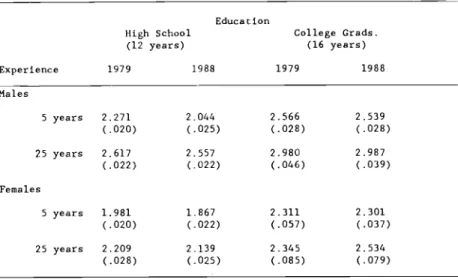
A. Workers in Large Firms (Multi-Establishment Firms with at least 1000

Employees)

Education

High School College Grads.

(12 years) (16 years) Experience 1979 1988 1979 1988 Males 5 years 2.271 2.044 2.566 2.539 (.020) (.025) (.028) (.028) 25 years 2.617 2.557 2.980 2.987 (.022) (.022) (.046) (.039) Females 5 years 1.981 1.867 2.311 2.301 (.020) (.022) (.057) (.037) 25 years 2.209 2.139 2.345 2.534 (.028) (.025) (.085) (.079)

8. Workers in Small Firms (Multi-Establishment Firms with less than

Employees or Single Establishment Firms)

1000

Education

High School College Grads.

(12 years) (16 yeats) Experience 1979 1988 1979 1988 Males 5 years 2.153 1.967 2.390 2.405 (.014) (.017) (.027) (.028) 25 years 2.486 2.409 2.789 2.845 (.023) (.026) (.048) (.053) Females 5 yearm 1.858 1.766 2.114 2.205 (.013) (.018) (.031) (.028) 25 years 2.014 2.003 2.144 2.410 (.018) (.021) (.079) (.058)

Table 3: continued

Note: Each estimate is from a separate cross-section regression for an educarion-experience-genderfirm size group of log real hourly earnings on a

linear spline of years of experience with a break every ten years, 2 race

dummy variables, and dummy variables for metropolitan area and part-time status. The education classes used are exactly 12 and 16 or more years of schooling; the experience classes are 0-19 and 20 or more years of potential experience. The regressions for college graduates include dummy variables for individual years of schooling. The estimates for each group are the predicted values of the log hourly earnings regression for that group evaluated at the indicated schooling and experience levels and for a full-time, white employee

living in a metropolitan area.

Sources: The data used are from the May 1979 and 1988 CPS Pension Supplement Surveys. The 1979 data include earnings for both the May 1979 and June 1979 Outgoing Rotation Groups. Earnings are deflated by the personal consumption

25

Cleveland provides further evidence of this phenomenon. Croshen finds that

occupational wage differentials within large private sector employers in

Cleveland, Cincinnati, and Pittsburgh did indeed expand substantially in the

1980s. This evidence indicates that the internal wage structures of large

private sector firms did change in the l980s and that government relative pay

rigidity is not something shared by all large bureaucratic organizations.

Finally the insensitivity of pay in the federal government to changes in

local labor market conditions documented in section III does not appear to be

a characteristic shared by large private sector employers in the United

States. Rebick (1990) finds for the 1979 to 1988 period that wages in small

firms (10 to 99 employees) , medium firms (100 to 999 employees) , and large

firms (1000 or more employees) in the private sector responded substantially

and similarly to changes in state unemployment rates.

B. Is Pay Rigidity A Characteristic of All Nonprofit Organizations?

A second potential explanation for the insensitivity of the government

internal wage structure to market changes in skill differentials is that such

behavior is characteristic of all "not-for-profit" organizations. This

hypothesis can be evaluated by examining whether wage differentials by skill

category behave similarly in the government and in private sector nonprofit

otganizations

19

We examine changes in wage differentials by education in the private

"for-profit", private nonprofit, and government sectors using data from the

19Furthermore, the "labor donations" model of Preston (1989) suggests that the supply of workers willing to accept a reduced wage to work for organizations that produce positive social externalities may be similar in

26

1979

and 1988 CPS outgoing rotation groups. Since the CPS does not identify

the whether workers are employed by nonprofit firms, a private sector worker is classified in the nonprofit sector if he or she works in a three-digit industry that has at least two-thirds of total employment in nonprofit firms. Following Preston (1989), we classified three-digit industries into the for-profit and nonfor-profit sectors on the basis of information reported in the 1977 census of service industries and tabulated by Rudney and Weitzman (1983). Private sector workers in all other industries are classified as part of the for-profit sector.

Table 4 presents estimates of the college/high school log wage premium

for males and females by sector in 1979 and 1988. The table shows that the

college wage premium increased substantially in the 1980s in both the private

for-profit and private nonptofit sectors. In contrast, the college/high

school

wage differential barely changed in the 1980s in the government

sector. Thus, relative pay rigidity in the 1980s is not apparent in the

private nonprofit sector and seems to be confined to public sector labor

markets.

C. The Role of Unionization

Freeman (1990) and others have argued that declining unionization may

have played an important role in rising skill differentials and wage

inequality in the United States in the 1980s. Since unions have largely

represented workers without college degrees in the private sector,

deunionization and losses of union wage premia are likely to reduce the wages

of less-educated workers relative to more-educated workers in the private

Table 4: College/High School Log Wage Differentials by Sector, 19791988a Group 1979 Males 1988 Change 1979-88 1979 Females 1988 Change 1979-88 Private Sector All 0.288 (0.006) 0.420 (0.006) 0.132 0.269 (0.007) 0.406 (0.006) 0.137 For-Profit sectorb 0.311 (0.024) 0.433 (0.030) 0.122 0.257 (0.022) 0.398 (0.023) 0.141 Nonprofit Sectorb 0.232 (0.036) 0.328 (0.037) 0.096 0.281 (0.014) 0.405 (0.014) 0.124 Government All 0.278 (0.011) 0.286 (0.011) 0.008 0.316 (0.009) 0.330 (0.010) 0.014

State and Local 0.270 0.277 0.007 0.354 0.366 0.012

Government (0.013) (0.013) (0.010) (0.011)

Federal 0.301 0.303 0.002 0.298 0.278 -0.020

Government (0.018) (0.019) (0.026) (0.025)

aEach estimate is from a separate cross-section regression for a

gender-sector group of log hourly earnings on dummy variables for individual years of schooling, a quartic in potential experience, two race dummy variables, a

dummy variable for metropolitan area status, and a dummy variable for

part-time status. The samples include workers with exactly 12 and with 16 or more years of schooling. Each reported estimate is the coefficient of the dummy variable for exactly 16 years of schooling with those with exactly 12 years of schooling as the base group. The numbers in parentheses are standard

errors.

bThe nonprofit sector includes private sector workers in the following

industries: hospitals; health services; elementary and secondary schools;

colleges and universities; libraries; educational services; museums, art galleries, and zoos; religious organizations; welfare services and welfare facilities; nonprofit membership organizations. Private sector workers in all other industries are classified as part of the for-profit sector. This

classification scheme is based on Appendix A of Preston (1989).

Source: The data are from the Full-Year 1979 and 1988 CPSs (Outgoing

27

unions compress wsges among organized workers in rhe privare secror. These

facrors suggesr rhar rhe high and relatively srable level of unionization in

the public sector since the mid-1970s may help explain much smaller increases in wage differentials by education in the public sector than in the private sector.

Our approach to assessing the role played by unionization in moderating

movements in skill differentials in the public sector relative to the private

sector is to compare changes in skill differentials in states with high and

low public sector unionization rates. Table 5 compares changes in the

college/high school log wage differential in the public and private sectors

from 1979 to 1988 for the ten states with the lowest and the ten states with

the highest public sector unionization rates in the early l98Os. We ranked

states according to their public sector union coverage rate in 1983 using tabulations from the CPS outgoing rotation groups reported by Curme, Hirsch,

and Macpherson (1990, Table 5, pp. 20-26). The public sector union coverage

rates in the high unionization states in 1983 ranged from 61.7 percent in

Maine to 73.5 percent in New York, while they ranged from 17.2 percent in

Georgia to 30.1 percent in Oklahoma in the low unionization states.

Table 5 indicates that the college wage premium increased substantially

more in the private sector than in the public sector in both groups of

states. Even in states with low public sector unionization rates, changes in

education differentials in the public sector were negative for men and quite

moderate for women in the 1980s. On the other hand, the table does indicate

that the college/high school wage differential is a bit lower in the public

sector in high unionization stares. Although unions may play a role in

Table 5: College/High School Log Wage Differentials for States

with High and Low Public Sector Union Coverage Ra