A Flow- and Packet-level Model of the Internet
Ramji Venkataramanan
Dept. of Electrical Engineering Yale University, USA
Email: [email protected]
Min-Wook Jeong,
Balaji Prabhakar
Dept. of Electrical Engineering Stanford University, USA Email:{minwook, balaji}@stanford.edu
Abstract—Several models of packet-switched networks have been proposed in the literature for analyzing network perfor-mance. There are two main types of models, called the packet-level and the flow-packet-level model, each making different assumptions about the operation of the network and providing different insights about its performance. While packet-level models are remarkably accurate, we find, from Internet packet traces and network simulations, that current flow-level models do not accurately model the Internet. This leads us to a new flow-level model that is more accurate and which, moreover, dovetails with a natural packet-level model to provide a complete description of the network. We validate our model via simulations and use it to provide a preliminary analysis of the Internet.
I. INTRODUCTION
It is important for network engineers to have good models to predict the performance of large networks like the Internet since the volume of traffic and the size of these networks make simulation impractical. Typical quantities of interest include flow transfer durations, throughput, queueing delay, queue-size distributions at the buffers etc.
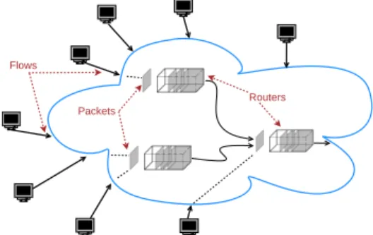
Figure 1 is a high-level depiction of a section of the Internet. Flows arrive at the edge of the network and send their packets into the core through access links. Each packet is routed through a series of routers (where it may be buffered and encounter queueing delays) until it reaches its destination. An end-to-end transport protocol governs the manner in which packets are injected into the core. TCP is the most commonly used transport protocol and regulates the sending rate of sources through a well-studied feedback congestion control mechanism. Each router in the core of the network sees an aggregate of packets sent by several flows, and is ignorant of the sending rate and other characteristics of individual flows. The models that have been proposed for the Internet can be classified broadly as either packet-level or flow-level models. Packet-level models such as those in [1]–[3], consider a fixed number of ‘long-lived’ flows, each with an infinite stream of packets. These packets are injected into the network according to a process that is governed by TCP’s congestion control mechanism. The packets are often approximated as fluid units to explicitly model the relationships between round-trip times, packet drop probabilities and rate-allocation among the flows. Consequently, they capture the role of buffers as well as queueing and propagation delays. Packet-level models are useful to estimate quantities such as queue sizes at buffers, and throughput. They have been heavily used to study the stability of congestion control algorithms (see [4], for example). Since only long-lived flows are considered, packet-level models are
Flows
Packets
Routers
Fig. 1: A high-level depiction of a network
static and do not capture flow-level dynamics such as flow durations or the number of active flows.
In flow-level models, such as those in [5], [6], flows are treated as finite-sized units of data, whose sizes are random and specified by a probability distribution. Flows arrive at the network according to an arrival process with a given distribution. The models aim to capture flow-level dynamics such as flow transfer durations and the number of active flows resulting from different flow bandwidth allocation procedures. It is assumed that there is an underlying mechanism that effects ‘statistical bandwidth sharing’, i.e., the rate of each flow is adjustedinstantaneouslybased on the available bandwidth on its path and the number of flows that it shares the bandwidth with at that instant. At each instant of time, a flow transmits data through the network according to the rate allotted to it. When a flow has been served completely, it departs. Flow-level models do not incorporate any packet-Flow-level details such as queuing delays at routers or propagation delays. Such details are abstracted away under the assumption of a ’time-scale separation’: the time-scale of the flow-level dynamics (flow duration) is assumed to be much larger than the time-scale of packet-level dynamics captured in models such as [1], [2].
Using a flow-level model, we would like to answer questions like: What are the number of active flows? What are the flow durations? What do the queues at the buffers look like? In this paper, we first investigate existing flow-level models, and compare their predictions with data from network simulations and internet traces. We find that they do not give accurate estimates of flow durations and the number of active flows, especially when link speeds are high. This is because in existing models, flows arrive and deliver data continuously for their whole duration, ignoring important effects created
by the congestion control protocol, queueing delays etc. We then propose a new flow-level model that is more accurate and which, moreover, dovetails with a natural packet-level model to provide a complete description of the network. The main contributions of this paper are as follows.
• In Section II, we examine the Bonald-Massoulie flow-level model from [5], and explain why it does not accurately capture certain key aspects of flow transfer in the Internet. We present network simulation and Internet trace analysis to illustrate these shortcomings.
• In Section III, we propose a flow- and packet-level model that is more accurate and captures the essential packet-level features of the network as well.
• We provide some preliminary analysis on the new model in Section IV and finally in Section V, validate our model by characterizing the aggregate packet traffic in the core of the Internet.
We note that the approach of packet-level models has been extended to estimate durations of short-lived TCP flows in [7], [8]. We also mention that a joint flow-level and packet-level stochastic network model, different from the one proposed here, was proposed recently in [9].
II. THEBONALD-MASSOULIEMODEL
The Bonald-Massoulie (B-M) flow-level model is one in which all the active flows on a link instantaneously share the link bandwidth according to a specified fairness criterion. For concreteness, we assume that the sharing takes place according to the max-min fairness criterion [10]. The specific details of the sharing mechanism are abstracted away. For illustration, first consider a single bottleneck link of capacity N µshared by flows arriving at rate N λ. Each flow has size S, drawn according to a distribution with mean E[S]. The queue is stable if the loadρ= N λN µ·E[S] is less than one.
The B-M model for this network corresponds to a processor sharing queue, where all the active flows share the link bandwidth equally. Hence, if the flows arrive according to a Poisson process, the number of active flows in the system is geometrically distributed with parameter ρ [11]. Thus the average number of active flows is 1−ρρ, and using Little’s law, one can show that the duration of a flow with size S
is N µ(1S−ρ). In other words, as the link speed and arrival rate increase proportional to N such that the load is fixed, the network just speeds up, and flow durations decrease as 1/N, while the average number of active flows remains the same.
Let us compare this with TCP flows with the same arrival characterstics sharing the bottleneck link. Due to the slow-start mechanism of TCP, the duration of a flow with S packets is at leastdlog2Seround-trip times. Since the propagation delay (which does not depend onN) is a lower bound on the round-trip time, this implies the duration of a TCP flow of size S
is an O(1)quantity, i.e., it does not go to zero, regardless of how large N is. In other words, the B-M flow-level model is too efficient- the flow durations for large N are not accurate since the model does not account for the inefficiency in the network created by the physical constraints of the protocol, viz., round-trip times.
Next consider the number of active flows in the network. As explained above, the average number of active flows in the B-M model is 1−ρρ, an O(1) quantity. In contrast, in a TCP network, flows arrive at rate N λ and stay in the system for
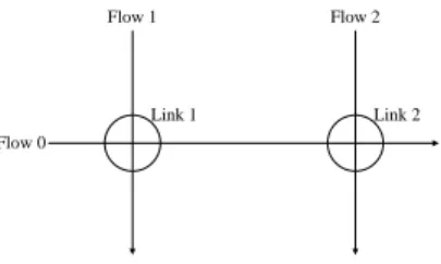
O(1) time, so there are Θ(N) active flows in the system at any given time. We now illustrate this by simulating a network with different routes and multiple bottlenecks.
Flow 0
Flow 2 Flow 1
Link 2 Link 1
Fig. 2: Two link network
Multiple Bottlenecks: Consider the network shown in Figure
2. There are three types of flows labeled 0,1, and 2, with arrival rates 0.05N, 0.04N and 0.04N flows/s, respectively. Type0flows pass through both link 1 and link2, while type
1 flows go through links1only, and type2 flows go through link 2 only. The size of each flow is drawn iid according to a heavy-tailed distribution with mean20packets. The service rate of each link is2N pkt/s, hence the load on each link is
90%. This example is used to model a network where the local and long distance traffic coexist.
In the B-M model, the instantaneous bandwidth allocated to each active flow is determined by the max-min fairness criterion. Thus the bandwidth allocation changes each time a flow arrives or departs the network. The first two rows of Table I show the average number of active flows of type 0 when the network of Figure 2 was simulated with instantaneous bandwidth sharing. We see that the number of active flows is roughly the same for bothN = 1andN = 1000.
The next two rows of Table I show the number of active flows of type0 for the same network configuration when the flows use TCP rather than instantaneous bandwidth sharing. (This was simulated using OMNET++ [12], with N = 1
corresponding to a link speed of 10Mbps.) The last two rows show the number of active flows in two internet traces - the LBL trace from 1994 (10 Mbps link) used in [13], and a recent trace from a 10Gbps link obtained from [14]. The ratio of the number of active flows in the 10Gbps link to the 10Mbps link is 155.1 for the simulation and 437.0 for the Internet traces. For the 10Mbps and 10Gbps Internet traces, the link utilizations are 3.51% and 26.04%, and the average packet sizes are 176.4B and 578.9B, respectively. Taking these two factors into account, the number of active flows is found to be proportional to the link speed. Thus the number of active flows in an Internet backbone link grows with the link speed, a feature not captured by the B-M model.
In a real network, there is also a limit on the maximum rate at which a flow can send its packets. This is reflected in the maximum receive window size imposed on any TCP connection. There are several reasons for this restriction. First, the constraints of the hardware, operating system and the
TABLE I: Average number of active flows
Setup Number of active flows
Bonald-Massoulie (N= 1) 18.7
Bonald-Massoulie (N= 1000) 17.5
TCP (OMNeT++, 10Mbps link speed) 72.3
TCP (OMNeT++, 10Gbps link speed) 11216.8
TCP (Internet trace, 10Mbps router, 1994) 327.7
TCP (Internet trace, 10Gbps router, 2009) 143192.4
application at the sender as well as the receiver impose an upper limit on the transmission rate of a flow. Secondly, if the TCP window grows very large, there are a large number of unacknowledged packets at any given time. This leads to a huge number of retransmissions when there is network congestion, resulting in throughput degradation. (In the OMNET++ simulation of Table I, the receive window was set to 64 packets.) Thus the access rate of a flow is limited in practice, even with plenty of link bandwidth available. To summarize, the B-M model has two main shortcomings:
• It ignores the closed control loop of the protocol, and assumes data can be sent continuously by a flow once it arrives at the network. This implies flow durations can get arbitrarily small as link speeds increase, contradicting the fact that a flow of sizeS packets is active for a minimum of log2S round-trip times.
• It does not account for the fact that access speed of a flow is limited by the maximum window size of TCP and cannot grow arbitrarily large. This imposes another lower bound on the flow duration of a large flow. Hence the B-M model does not capture the role of round-trip times and queueing in the network. It is also difficult to use the model to make predictions on large, unstructured network topologies. We now propose a flow- and packet-model that attempts to address these shortcomings.
III. THEFLOW-ANDPACKET-LEVELMODEL
Figure 3 shows the network of Figure 1 with flows arriving at backbone link i at the rate of N λi, i = 1,2,3. Link i is
represented by a single-server queue with service rate N µi
packets/s. N is the scaling parameter to capture the growth in arrival rates and link speeds. Each flow at the edge is assigned a separate server (representing the access link) which which serves it packet by packet. The served packets enter the queue corresponding to the backbone link. At the access link, different packets of a flow may receive different rates of service, depending on the congestion encountered at the downstream queue by the previous packets. The mechanism to effect this is described in the sequel.
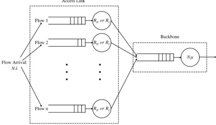
Let us first consider a simple network with a single back-bone link. Suppose flows arrive at the edge according to a Poisson process of rate N λ, and share the downstream link of capacity N µ. Each flow consists of a random number of packets S, drawn independently according to a known heavy-tailed distributionPS with meanE[S]. The sizes of the
individual packets are assumed to be iid according a known distribution. The system is depicted in Figure 4.
N µ1 N µ2 N µ3 N λ2 N λ1 N λ3
Fig. 3: Flow- and Packet-level model for network of Figure 1
We now specify the mechanism which controls the rate of service the packets of a flow receive at the access link. Recall that the instantaneous rate (or congestion window) of a TCP flow depends on the level of congestion encountered by the previous packets of the flow. This signalling mechanism is modeled as follows. The service rate of a flow at the edge can take one of two values - Rl or Rh, where 0 < Rl <
Rh. A flow starts being served at rate Rl. The service rate
is set to Rh if the flow encounters no drops for a certain
number of consecutive packets, sayC. This models the slow-start phase of TCP. When the buffer of the downstream queue hasqpackets, an incoming packet is dropped with probability
f(q), wheref(q)is a non-decreasing function ofq. If a packet is dropped and the current service rate of the flow isRh, the
rate is instantly reduced toRl. This captures the dynamics of
the TCP connection, while maintaining the parsimony of the model. As a first step, we ignore delays in the feedback loop and assume acknowledgements and drops are instantly known at the edge. The access rates Rl andRh are assumed to be
O(1)to reflect the fact that TCP imposes a limitation on the maximum window size of a connection.
Flow 1 Flow n Flow 2 Flow Arrival: N H L R or R N Access Link Backbone H L R or R H L R or R
Fig. 4: Flow- and Packet-level model for a single bottleneck link
We note that this network is stable as long asλE[S]< µ. As
N grows, we now show that this model qualitatively captures the important features of a TCP network. First, consider flow durations. In the model, a flow at the edge starts off being
served at the low rateRl. Hence the completion time of flow
with S packets is at least RC l +
S−C
Rh if S ≥ C, and
S
Rl,
otherwise. SinceRldoes not scale withN, the flow durations
do notgo to zero as link bandwidth grows withN, consistent
with the behavior of a TCP flow. (Recall from the previous section that a lower bound on the duration of a TCP flow with
S packets islog2S round-trip times.)
Next, consider the number of active flows in the model. Since flows arrive at rate N λ and flow durations are O(1), the number of active servers at the edge is Θ(N). This is consistent with the scaling behavior of a network with TCP flows, as illustrated in the previous section.
Finally, we consider the aggregate packet traffic entering the downstream queue. The arrival rate of packets to the queue is N E[S]λ. This grows linearly with N, while the packet processing time at the downstream queue decreases as
1
N µ. In other words, as N increases, the fluctuations in the
downstream queue become more rapid, but the average load remains the same.
The inter-arrival time at the downstream queue between two successive packets of the same flow is at least R1
h sec. Since the downstream queue fluctuates Θ(N) times per second, the number of fluctuations between the arrival times of two packets of any flow is at least Θ(N
Rh) = Θ(N). Since the
queue fluctuates a large number of times between the arrivals of the two packets, we expect the queue sizes encountered by different packets of the same flow to be independent. This intuition is verified by simulations in the next section.
IV. THEAGGREGATEPACKETPROCESS FORLARGEN A. The Packet Drop Process
Consider the following thinned version of the original flow arrival process. Pick any K > 0 and assume each arriving flow is ‘tagged’ with probability KN. Since the original arrival process is Poisson with rateN λ, the arrival process of tagged flows is a Poisson process of rate Kλ. We refer to packets belonging to tagged flows as tagged packets. LetPK(t)be the
counting process corresponding to arrivals of tagged packets at the downstream queue. LetMK(i)be an indicator function
which is equal to 1 if the ith tagged packet arriving at the downstream queue is dropped, and 0 otherwise. ThusMK(.)
is the binary packet drop process corresponding to packets from the tagged flows only.
The arrival rate of packets at the downstream queue is
N λE[S], while the arrival rate of the tagged packets is
λKE[S] Thus the number of untagged packets arriving be-tween any two successive tagged packets is Θ(N−K
K ). If we
keep K fixed and let N grow, the queue fluctuates a large number of times between the arrivals of two successive tagged packets, and we expect the queue sizes encountered by these packets to be independent. This intuition is summarized by the following conjecture.
Conjecture: For a fixed K, MK(.) converges to an iid
Bernoulli process as N → ∞.
We do not have a proof of the conjecture yet, but experi-mentally verify it below.
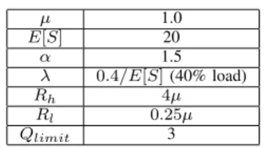
Simulation Set-up: Each flow is chosen according to a
heavy-tailed Pareto distribution with parameter α and mean
E[S]. The packet drop probability f(q)is1 if the queue-size
Q > Qlimitand zero otherwise. The value of all the quantities
used in the simulation are given in Table II. TABLE II: Simulation parameters
µ 1.0 E[S] 20 α 1.5 λ 0.4/E[S](40% load) Rh 4µ Rl 0.25µ Qlimit 3
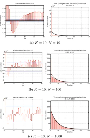
We fixK, and observe the correlation inMK(.)for different
values of N. We plot two quantities: 1) The autocorrelation function ofMK normalized by the variance and, 2) the pmf of
the spacing between successive ones (drops) in MK. For any
iid Bernoulli process, the normalized autocorrelation function is the Kronecker delta function, and the pmf of the time spacing is geometric.
Figure 5 shows these two plots for increasing values of
N with K = 10. When N = K = 10, every flow is tagged and MK(.) is the drop-process corresponding to all
arriving packets. In this case, we expect MK to have a
large auto-correlation for small delays since successive packets will encounter similar levels of congestion. As N increases, there is an increasing number of untagged packets arriving between two successive tagged packets. Hence the queue sizes encountered by successive tagged packets look more independent asN increases.
B. The Aggregate Packet Arrival Process
Based on the conjecture, we prove the following result about the aggregate packet process from tagged flows entering the downstream queue.
Theorem 1: Let PK(t) be the arrival process of tagged
packets at the downstream queue. Define
AK(t),PK(
t K).
Under the conjecture that the drop processMK(.)is iid,AK(t)
converges weakly to a Poisson process of rateE[S]λasK→ ∞.
The proof of the Theorem is given in the Appendix. Note that AK(t) is the arrival process of tagged packets on a
time-scale expanded by a factor of K. We demonstrated by simulation that when N K, MK(.) is well-approximated
by an iid Bernoulli process. We can satisfy the conditions of the theorem by letting N go to ∞ faster thanK (N =K2, for example).
We note that a result related to Theorem 1 is found in [15]. In [15], a fixed number N of infinitely long-lived flows send packets into a single-server queue according to a stationary point process with constant rate. It is shown that asN → ∞, the queue behaves as if it were fed by a Poisson input process. In our model, we have short-lived flows whose sending rates depend on the congestion encountered in the downstream
0 10 20 30 40 −0.03 −0.02 −0.01 0 0.01 0.02 0.03 lag autocorrelation Autocorrelation K=10, N=10 0 20 40 60 80 100 0 0.5 1 1.5 2 2.5 3 3.5 x 10⁴
Time spacing between successive packet drops K=10, N=10 Spacing # of occurrence (a)K= 10,N= 10 0 10 20 30 40 −8 −6 −4 −2 0 2 4 6 8 x 10⁻³ lag autocorrelation Autocorrelation K=10, N=100 0 20 40 60 80 100 0 1000 2000 3000 4000 5000 6000 7000
Time spacing between successive packet drops K=10, N=100 Spacing # of occurrence (b)K= 10,N= 100 0 10 20 30 40 −5 0 5 x 10⁻³ lag autocorrelation Autocorrelation K=10, N=1000 0 20 40 60 80 100 0 500 1000 1500 2000 2500
Time spacing between successive packet drops K=10, N=1000
Spacing
# of occurrence
(c)K= 10,N= 1000
Fig. 5: Analysis of the packet drop process MK()
queue. In both these results, statistical multiplexing of packets from the different flows is responsible for smoothing of the aggregate packet process seen by the downstream queue.
V. DISCUSSION
Figure 3 provides a parsimonious model of a large network in terms of the arrival rates of the flows and the link capacities. The parameters governing the access rate - RH, RL, andC
-can be adjusted to capture the essential features of TCP: the slow-start mechanism, the growth of the congestion window, and the maximum window size. For the simple case of a single bottleneck link, Theorem 1 says that if we observe the aggregate packet traffic of any subset of arriving flows, it resembles a Poisson process if the link speed is sufficiently large. In fact, simulations and analysis of Internet traces (described below) suggest that a stronger result may hold: the aggregate packet traffic into the downstream queue, when suitably scaled, converges to a Poisson process as N → ∞. If such a result were true:
• The network of routers becomes a Jackson network [16] as N → ∞, leading to a product-form decomposition of the queue-size distributions. The queue-size distributions at the buffers could then be easily estimated.
• From the queue size-distribution and the function f(q)
used for dropping, the packet drop probability can be computed. Using this, one can compute the fraction of
0 20 40 60 80 100 −15 −10 −5 0 Exponentiality test: lbl_pkt_4 ln ( P(X>x) ) x (milliseconds) (a) LBL trace (1994) 0 20 40 60 80 100 −15 −10 −5 0 Exponentiality test: 20090331_060100_0 ln ( P(X>x) ) x (microseconds) (b) OC192 trace (2009)
Fig. 6: Distribution of the packet interarrival time
0 50 100 150 200 250 300 350 400 0.02 0.04 0.06 0.08 0.1 0.12 0.14 Autocorrelation : lbl_pkt_4 Lag k (>=1)
Norm. auto−corr. at lag k
(a) LBL trace (1994) 0 50 100 150 200 250 300 350 400 −0.01 0 0.01 0.02 0.03 0.04 0.05 0.06 Autocorrelation : 20090331_060100_0 Lag k (>=1)
Norm. auto−corr. at lag k
(b) OC192 trace (2009)
Fig. 7: Autocorrelation of the packet interarrival times
packets of a given flow that are served at the higher rate
Rh. Using this, the flow durations can be estimated.
There have been extensive efforts to characterize the Internet packet traffic based on trace analysis. Early studies such as [13], [17] found that Internet traffic exhibits long-range dependent behavior, characterized by the sustained correlation of packet counts or packet interarrival times over a long period of time. In contrast, more recent studies such as [18], [19] find evidence that the Internet traffic exhibits Poisson-like behavior, especially on short time scales.
The model of Section III pinpoints the reason for this change in internet traffic characteristics. In the early 90s, both flow arrival rates and link speeds were quite low. In our model, this corresponds toN being small, and hence the aggregate packet traffic does not exhibit Poisson behavior. Both backbone link speeds and flow arrival rates have increased more than a thousand-fold since the90s, corresponding to a much largerN
in our model. Thus there is increased multiplexing of packets from different flows, leading to smoothing of the aggregate packet process.
For illustration, we analyze two traces: 1) an LBL trace from 1994 that was used in [13] to show long-range dependence of internet traffic, and 2) a trace from an OC192 (10 Gps) link in 2009, obtained from CAIDA [14]. Recall that for a Poisson process, inter-arrival times are independent and exponentially distributed. We test the packet inter-arrival times of the traces for both of these properties. Figure 6 plots lnP(X > x)
against x, where X is the inter-arrival time and P(X) its empirical distribution from the traces. For the 2009 OC192
trace, the plot is close to a straight line, indicating that the distribution of the packet inter-arrival time is exponential. The plot is not a straight line for the 1994 LBL trace. Figure 7 plots the autocorrelation of the packet inter-arrival times (normalized by the variance) for various values of lag k. For LBL trace, autocorrelation does not go to zero even for large values ofk, showing the long range dependence of the inter-arrival time process. For the OC192 trace, autocorrelation is very small for large k, and takes both positive and negative values. The two tests indicate that the distribution of packet inter-arrival times for the OC192 traces resemble an i.i.d exponential random variable much more than the distribution for the LBL trace. Finally, we note that [18] contains extensive trace analysis showing Poisson-like behavior of packet traffic for OC48 (2.5Gbps) backbone links.
An important factor we have ignored in this paper is the role of delay (round-trip time) in the feedback loop. It is important to study how lags affect the smoothing of the packet process caused by multiplexing of packets from different flows. The ultimate goal is to prove a convergence result for the aggregate packet process entering the downstream queue without the help of the conjecture. The challenge here is to explicitly take into account the instantaneous correlation in the access rates of the different flows.
REFERENCES
[1] V. Misra, W. Gong, and D. Towsley, “Fluid-based analysis of a network of AQM routers supporting TCP flows with an application to red,” in
In Proc. of ACM SIGCOMM, 2000.
[2] J. Mo and J. Walrand, “Fair end-to-end window-based congestion
control,” IEEE/ACM Trans. Networking, vol. 8, no. 5, pp. 556–567,
2000.
[3] F. P. Kelly, A. Maulloo, and D. Tan, “Rate control in communication
networks: shadow prices, proportional fairness and stability,”Journal of
the Operational Research Society, vol. 49, pp. 237–252, 1998.
[4] R. Srikant,The Mathematics of Internet Congestion Control. Birkhauser,
2004.
[5] T. Bonald and L. Massouli´e, “Impact of fairness on internet
perfor-mance,” inIn Proc. of ACM SIGMETRICS, pp. 82–91, 2000.
[6] S. B. Fredj, T. Bonald, A. Proutiere, G. R´egni´e, and J. Roberts, “Statistical bandwidth sharing: A study of congestion at flow level,” inIn Proc. of ACM SIGMETRICS, 2001.
[7] N. Cardwell, S. Savage, and T. Anderson, “Modeling TCP latency,” in
In Proc. of IEEE INFOCOM, 2000.
[8] U. Ayesta, K. Avrechenkov, E. Altman, C. Barakat, and P. Dube,
“Multilevel approach for modeling short TCP sessions,” inIn Proc. of
ITC-18, Berlin, 2003.
[9] C. Moallemi and D. Shah, “On the flow-level dynamics of a
packet-switched network,” inIn Proc. of ACM SIGMETRICS, 2010.
[10] D. Bertsekas and R. Gallager,Data Networks. Prentice Hall, 1987.
[11] L. Kleinrock,Queueing Systems, vol. 2. J. Wiley and Sons, 1975.
[12] “OMNeT++ network simulator.” http://www.omnetpp.org/.
[13] V. Paxson and S. Floyd, “Wide-area traffic: The failure of poisson
modeling,”IEEE/ACM Trans. Networking, pp. 226–244, June 1995.
[14] C. Walsworth, E. Aben, K. Claffy, and D.
Ander-sen, “The caida anonymized oc192 traces 2009.”
http://www.caida.org/data/passive/passive 2009 dataset.xml, 2009. [15] J. Cao and K. Ramanan, “A poisson limit for buffer overflow
probabil-ities,” inIn Proc. of IEEE INFOCOM, 2002.
[16] F. P. Kelly,Reversibility and Stochastic Networks. Wiley, 1979.
[17] W. E. Leland, M. S. Taqqu, W. Willinger, and D. V. Wilson, “On the
self-similar nature of ethernet traffic,”IEEE/ACM Trans. Networking,
pp. 1–15, February 1994.
[18] T. Karagiannis, M. Molle, M. Faloutsos, and A. Broido, “A nonstationary
poisson view of internet traffic,” inIn Proc. of INFOCOM, 2004.
[19] Z.-L. Zhang, V. J. Ribeiro, S. Moon, and C. Diot, “Small-time scaling
behaviors of internet backbone traffic: An empirical study,” inIn Proc.
of INFOCOM, 2003.
[20] D. Daley and D. Vere-Jones,An Introduction to the Theory of Point
Processes. Springer, 2003.
APPENDIX
PROOF OFTHEOREM1
We will first give the proof for fixed flow-sizeS, and then extend to arbitrary flow-size distributions.
Deterministic flow sizeS
The arrival process of tagged packets to the downstream queuePK(t)can be written as
PK(t) =PK1(t) +PK2(t) +. . .+PKS(t), t≥0 (1)
wherePKj(t)is the counting process corresponding to arrival of the jth packet of each tagged flow for j = 1, . . . , S. and hence AK(t) =PK1( t K) +P 2 K( t K). . .+P S K( t K), t≥0 (2)
Forj= 1, . . . , S, letRjbe the rate at which thejth packet
of a given flow is served at the access link;Rj can take value
either Rh or Rl. By assumption, there is a fixed probability
pof a tagged packet getting dropped which is independent of the current access rates of all the tagged flows. This induces a stationary joint distributionP(R1, R2, . . . , RS)which governs
the access rates of the S packets in each flow. This joint distribution is determined by p and the congestion control algorithm. Denoting the Poisson flow arrival process of tagged flows by TK(t), observe that PK1(t) is a process formed by
shifting to the right each arrival inFK independently, where
the shifts are i.i.d realizations of R1
1, with R1 ∼ P(R1). (P(R1)is the marginal from the joint distribution.) From [20, Problem 2.3.4 (b)],PK1(t)is a Poisson process with rateKλ.
Similarly, for 1 ≤ i ≤ S, Pi
K(t) is a process formed
by shifting to the right each arrival in FK independently,
where the shifts are i.i.d realizations of R1
1 +. . .+ 1
Ri, with
(R1, . . . , Ri) ∼ P(R1, . . . , Ri). Hence PKi (t) is a Poisson
process of rate Kλ for 1 ≤ i ≤ S. We now show that
AK(t) defined in (2) satisfies both the stationary increments
and independent increments properties as K→ ∞.
Stationary increments. Consider the number of points of the process AK(t) in the interval t ∈ (a, a+ ∆), denoted
AK(a, a+ ∆). This is equal to the sum of the number points
of P1
K, . . . , PKS that occur in the interval( a K, a+∆ K ). Pr(AK(a, a+ ∆) =n) = n X kS=0 n−kS X kS−1=0 . . . n−(kS+...+k3) X k2=0 Pr PKS a K, a+ ∆ K =kS, . . . , PK1 a K, a+ ∆ K =n−(kS+. . .+k2) . (3)
Since PKS is a Poisson process of rate Kλ, we can write the above using conditioning as
Pr(AK((a, a+ ∆)) =n) = n X kS=0 n−kS X kS−1=0 . . . n−(kS+...+k3) X k2=0 e−λ∆(λ∆)kS kS! · ·Pr PKS−1 a K, a+ ∆ K =kS−1· |PKS a K, a+ ∆ K =kS . . . ·Pr PK1 a K, a+ ∆ K =n−(kS+. . .+k2)|PKS a K, a+ ∆ K =kS, . . . (4)
Consider the first conditional probability term in the above equation. Let thekS points inPKS (
a K, a+∆ K ) occur at times t1, t2, . . . , tkS, a
K < ti < a+∆K . Let the corresponding Sth
packet service times for these points be D1, D2, . . . , DkS, respectively. Note that D1, D2, . . . , DkS are independently distributed∼ 1
RS.
Then, the points in PS
K ( a K, a+∆ K ) exactly correspond to
kS points in the processPKS−1(t)at times(t1−D1, . . . , tk−
DkS). Since 1 Rh ≤Di ≤ 1 Rl , ∀i,
thesekpoints all lie within the interval(a
K− 1 Rl, a+∆ K − 1 Rh). If a+ ∆ K − 1 Rh < a K, (5) then(a K, a+∆ K )and( a K− 1 Rl, a+∆ K − 1
Rh)are disjoint intervals. Thus if (5) holds, the points of AK((a, a+ ∆))fromPKS and
PKS−1 correspond to points of PKS−1 in disjoint intervals of time. Let E denote the event that Rh < K∆, i.e., (5) holds.
Then we have Pr PKS−1(a K, a+ ∆ K ) =kS−1|P S K( a K, a+ ∆ K ) =kS =Pr E, PKS−1(a K, a+ ∆ K ) =kS−1|P S K( a K, a+ ∆ K ) =kS +Pr Ec, PKS−1(a K, a+ ∆ K ) =kS−1|P S K( a K, a+ ∆ K ) =kS . (6) We have Pr PKS−1( a K, a+ ∆ K ) =ks−1|E, P S K( a K, a+ ∆ K ) =ks =e −λ∆ (λ∆)ks−1 (ks−1)!
because conditioned on E, the points in PS
K(
a
K,
a+∆
K ) all
correspond to points of PKS−1 in a disjoint interval from
(a
K,
a+∆
K ).
Also note that for any fixed ∆,Rh < K∆ for large enough
K. Hence, lim K→∞P(E) = 1 and (6) becomes lim K→∞Pr PKS−1(a K, a+ ∆ K ) =ks−1|P S K( a K, a+ ∆ K ) =ks = e −λ∆(λ∆)ks−1 ks−1! (7) We can similarly find the limiting value of each term in the expansion (4) to obtain lim K→∞Pr(AK(a, a+ ∆) =n) = n X kS=0 . . . n−(kS+...+k3) X k2=0 e−λ∆(λ∆)ks ks! ·e −λ∆(λ∆)ks−1 ks−1! . . .e −λ∆(λ∆)n−ks−...−k2 (n−ks−. . .−k2)! =e −Sλ∆(λ∆)n n! X k1,...,ks: Pk i=n n k1k2. . . kS =e −Sλ∆(Sλ∆)n n! . (8) ThusAK(a, a+ ∆)has a Poisson distribution with parameter ∆ for alla, which is the stationary increments property.
Independent Increments. Consider two disjoint intervals
(b, b+δ)and(a, a+∆), witha > b+δ. We need to show that
AK((a, a+ ∆))is independent ofAK((b, b+δ))asK→ ∞. We have AK(a, a+ ∆) =PK1( a K, a+ ∆ K )+ . . .+PKS−1(a K, a+ ∆ K ) +P S K( a K, a+ ∆ K ), AK(b, b+δ) =PK1( b K, b+δ K )+ . . .+PKS−1( b K, b+δ K ) +P S K( b K, b+δ K ). (9) We now show that each term inAK(a, a+ ∆)is independent
of AK(b, b+δ)as K→ ∞. ConsiderPKS( a K, a+∆ K ). • PKS(Ka,a+∆K ) is independent of PS K( b K, b+δ K ) for all K
since they correspond to disjoint intervals of the Poisson processPKS(t).
• As before,let the points in PKS Ka,a+∆K occur at times
t1, t2, . . . , tkS,
a
K < ti<
a+∆
K and let D1, D2, . . . , DkS be the corresponding Sth packet service times for these points . Then these exactly correspond to kS points in
the processPKS−1(t)at times(t1−D1, . . . , tk−DkS). If
a+ ∆ K − 1 Rh < b K, (10) then (b K, b+δ K ) and ( a K − 1 Rl, a+∆ K − 1 Rh) are disjoint intervals. (10) is equivalent toRh< a+∆K−b, which holds
for any finite ∆, a and b (a > b) for large enough K. Thus PS K( a K, a+∆ K )is independent ofP S−1 K ( b K, b+δ K )as K→ ∞.
Similarly, we can show that each term in the expansion (9) of
AK(a, a+ ∆) is independent of each term of AK(b, b+δ)
as K → ∞. This completes the proof that AK(a, a+ ∆) is
independent ofAK(b, b+δ)for all sufficiently largeK. Random Flow-sizes
Let pi denote the probability that a flow has size i, so
that E[S] = P
iipi. Denote by PKi(t) the packet-departure
process corresponding to tagged flows with size i. Then the packet departure processPK(t)can be written as
PK(t) = X i PKi(t) (11) and hence AK(t) = X i AKi(t) = X i PKi(t/K). (12)
The processes{PKi(.)}i are mutually independent because
the assumption of iid drops ensures that the (time-varying) access rate of each tagged flow is independent of all other tagged flows.
The arrival process of tagged flows of size i is a Poisson process of rate Kpiλ(thinning a Poisson process of rateKλ
by a factor of pi). From the result proved above for the
deterministic case, AiK(t) converges to a Poisson process
of rate ipiλ. Thus in the limit K → ∞, (12) is a sum of
independent Poisson processes with theith process in the sum have rate ipiλ. Thus, limK→∞AK(t) is a Poisson process
with rate P