Dis cus si on Paper No. 13-099
Cyclically Neutral
Generational Accounting
Holger Bonin, Concepció Patxot,
and Guadalupe Souto
Dis cus si on Paper No. 13-099
Cyclically Neutral
Generational Accounting
Holger Bonin, Concepció Patxot,
and Guadalupe Souto
Download this ZEW Discussion Paper from our ftp server:
http://ftp.zew.de/pub/zew-docs/dp/dp13099.pdf
Die Dis cus si on Pape rs die nen einer mög lichst schnel len Ver brei tung von neue ren For schungs arbei ten des ZEW. Die Bei trä ge lie gen in allei ni ger Ver ant wor tung
der Auto ren und stel len nicht not wen di ger wei se die Mei nung des ZEW dar.
Dis cus si on Papers are inten ded to make results of ZEW research prompt ly avai la ble to other eco no mists in order to encou ra ge dis cus si on and sug gesti ons for revi si ons. The aut hors are sole ly
Cyclically Neutral Generational Accounting*
Holger Bonin°Centre for European Policy Research (ZEW), University of Kassel and IZA Concepció Patxot
Universitat de Barcelona Guadalupe Souto
Universitat Autònoma de Barcelona
Abstract
This paper introduces a methodological innovation into Generational Accounting. By incorporating cyclically-adjusted balances into the forward-looking budget projections underlying the concept we isolate pure policy effects, which render comparisons of the fiscal sustainability indicators obtained across time and countries truly meaningful. We also show that a demographic effect and a debt effect may bias fiscal sustainability measures over time, and establish a routine to control for these effects in the generational accounting framework. An empirical application for Spain illustrates that our proposed decomposition of indicators is empirically relevant. Standard generational accounting suggests that fiscal sustainability in Spain improved substantially in preparing for EMU. However, calculation of the pure policy effects reveals that this has not been the case.
Keywords: Fiscal Sustainability, Demographic Ageing, Cyclically-Adjusted Budget
Balance, Spain
JEL Classification: E62, H55
*This work received institutional support from the Spanish Science and Technology System (projects ECO2009-10003 and ECO2008-04997/ECON), the Catalan Government Science network (projects SGR2009-600 and SGR 2009-359) as well as from XREPP- Xarxa de Referència en Economia i Polítiques Públiques. We are grateful to two anonymous referees for helpful comments.
1. Introduction
The Stability and Growth Pact (SGP) was designed to draw the attention of decision-makers to the development of public deficits and debt. However, the ad-hoc deficit and debt ceilings in the Economic and Monetary Union specified in the Treaty of Maastricht may well not be very informative with regard to the actual stance of fiscal policy – a fact suddenly uncovered all too clearly by the current European debt crisis.
In the short term, government revenue and expenditure levels vary over the business cycle even when the underlying fiscal policy parameters are constant. An exact picture of debt policies under way thus requires eliminating cyclical effects from government balances. There are several approaches to disentangle cyclical and structural components in current government balances. These methods generally build upon econometric analysis of correlations between government revenue and expenditure, and some measure of economic activity. The common feature is that de-trending is based on past government experiences. Hence we may speak of backward-looking techniques. Larch and Turrini (2009) review the main shortcomings encountered in implementing this technique as a tool to assess fiscal surveillance.
Furthermore, in the medium and long term, current deficits or surpluses may turn out to be more or less sustainable when demographic dependency rates deteriorate. This means that for constant and even for cyclically neutral fiscal parameters, a given budgetary imbalance can develop into larger or smaller deficits in the future depending on the composition of government expenditure and revenue, in particular by age. In assessing current fiscal policy, according to the neoclassical model of debt in a general equilibrium framework, intertemporal sustainability matters, since it affects consumption patterns of rational individuals optimizing over the life-cycle. The various methods for evaluating fiscal sustainability available from the literature, surveyed by Balassone and Franco (2001), are generally forward-looking. The most advanced of these techniques develop projections for the future path of primary imbalances and generate estimates of the fiscal policy adjustments required to stabilize government debt at some predetermined rate of GDP. Balassone et al. (2009) present different quantitative indicators to assess the sustainability of public finances in the euro area against the backdrop of ageing.
Where measures of fiscal sustainability have been repeatedly calculated, the experience is that the results can vary substantially over very short periods. However, the swings are only partly due to structural changes in fiscal policy. As the primary imbalance at the start of the projections varies over the business cycle, inter-temporal fiscal imbalances tend to fluctuate cyclically, too. In order to determine whether fiscal policy is actually expansionary or contractionary, it is therefore informative to separate the cyclical and structural components in fiscal sustainability measures. Conceptually this is also a prerequisite for meaningful cross-country comparisons, as individual countries are likely at different stages of the business cycle in a given year.
In this paper, we expand the standard forward-looking analysis of fiscal imbalances by integrating backward-looking de-trending procedures. Specifically, we incorporate the method by Girouard and André (2005), which is the basis for the standardized measure of the cyclically-adjusted budget balance reported by the
European Commission, into Generational Accounting (GA), a widespread framework
for applied fiscal sustainability analysis in a changing demographic environment developed by Auerbach, Gokhale and Kotlikoff (1991, 1992).
This approach is linked to previous work by Hagist and Benz (2008) who applied HP-filters in order to obtain neutral budget aggregates for a generational accounting analysis of fiscal sustainability in Germany. However, our proposed method in addition establishes routines to control for what we call a demographic effect and a debt revaluation effect. This paper uncovers that these two effects, in addition to the cycle effect, may blur the pure policy effect, if one compares the year-to-year changes in the established generational accounting indicators of fiscal sustainability.
Our empirical application deals with Spain, where public deficits showed a remarkably strong decline during the second half of the 1990s. In preparing for EMU the deficit-to-GDP ratio fell from 7.2 per cent in 1995 to 0.1 per cent in 2004. It continued to improve, reaching a surplus between 2005 and 2007 (1.3, 2.4 and 1.9 per cent, respectively), reversing only in 2008 because of the financial and housing market crises. As a result, according to conventional GA measures, it seems that sustainability of Spanish fiscal policy has improved by a wide margin in preparing for EMU. However, if one relies on cyclically neutral generational accounting, the picture becomes quite different: as we show in Section 3, some signals of the current fiscal sustainability problems were already present in the period 1995-2005.
The remainder of the paper is organized as follows. In the next section, we outline the standard GA method and the modifications needed in order to disentangle pure policy effects from the cycle and other effects hiding them. Section 3 illustrates the method by means of an application to the Spanish case over the period 1996-2005. Finally, Section 4 is devoted to conclusions and further remarks.
2.
Isolating Cyclical and Structural Components in Fiscal
Imbalances
This section first presents the conventional practice of GA, which measures the intertemporal fiscal imbalance in government budgets. We demonstrate that the fiscal sustainability measures generated tend to perpetuate initial business cycle conditions. Next, we give a short introduction to the method by Girouard and André (2005) of adjusting the components of current fiscal imbalances for business cycle effects. Finally, we give an account of the method proposed to disentangle the true change in sustainability from other factors influencing the GA calculations.
2.1. Conventional Generational Accounting
Auerbach, Gokhale and Kotlikoff (1991, 1992) proposed GA to assess redistribution between current and future generations through public debt in the face of demographic changes.1 The method is based on the old theoretical notion that debt cannot increase at a faster rate than GDP for ever since otherwise, in a dynamically efficient economy, the taxes needed to service interest payments converge to an infinite value (Domar, 1944). Specifically, GA defines a sustainable fiscal policy as one capable of meeting the intertemporal budget constraint of the government in absolute terms:
t t t t t t S r D
0 0 0 (1 ) (1)Where St is the primary public surplus in period t, Dt0 is the value of public debt in the base period t0, and r is the discount rate applied to take the value of future payments
back to the base period.2 In other words, a sequence of future primary surpluses is considered sustainable, if its aggregate present value is sufficient to pay for the initial level of government liabilities. Most fiscal sustainability measures in the literature start from this or a closely related definition of fiscal sustainability. For example, the tax-gap indicator proposed by Blanchard et al. (1990), the most prominent alternative to the fiscal sustainability measures of GA, is based on the sustainability condition that the aggregate present discounted value of the ratio of primary deficits to GDP is equal to the negative of the current level of debt to GDP. This condition is weaker than the one set out before – it allows any positive debt-to-GDP ratio in absolute terms as long as it converges to zero in present value terms. In contrast, GA requires that the debt-to-GDP ratio converges to zero in absolute terms over an infinite time horizon.
No matter which sustainability concept is applied, a major difficulty is obtaining a meaningful long-term projection for primary imbalances. In order to capture the effect of demographic changes on public budgets, GA groups the primary surplus by cohort. Let Pjt be the number of the population of age j in period t, J the maximum age and jt
the average per-capita net tax payment by persons of age j in period t, then
J j jt jt t P S 0 .3 (2)Testing the sustainability condition (1) hence requires a population forecast and a forecast of age-related per capita net tax payments. For the former, generational accountants normally refer to official demographic projections. With regard to the latter, the basic concept is to assume that age-related per capita revenue and spending levels stay constant from the base period in terms of real per capita GDP:
0 0 t t jt jt (1 g) (3)
Where g is the per-capita real GDP growth rate. The vector of age-specific net tax payments in the base period is obtained from micro data on age-related tax payments
2 There is no unique approach to the debt measure. The choice is between gross and net values, market
and face values. See Baldassare and Franco (2001) for a discussion of the various possibilities.
3 Net tax payments are defined as the sum of taxes paid minus the total of transfers received. Since
Raffelhüschen (1999), net taxes generally also include government consumption. It is treated as a non-age-related expenditure. This means that for each age group the level of net taxes shifts by a constant amount.
and benefit receipts, which are rescaled so that individual net tax payments weighted by cohort size add up to the actual primary imbalance in the base period as measured by the national accounts.
If the primary imbalances computed on the basis of (2) and (3) violate the intertemporal financing condition (1), fiscal policy is unsustainable. To finance the difference between the absolute value of initial debt and aggregate primary surpluses, the so-called sustainability gap (SG), fiscal policy must be adjusted at some future
point in time. For example, if the sustainability gap is positive, per-capita revenue has to increase, or per-capita spending has to fall relative to what is predicted on the basis of the initial fiscal parameters. In this respect, the sustainability gap constitutes an intertemporal financial liability of the government. We will call fiscal policy that increases (decreases) the sustainability gap expansionary (contractionary).
In principle, evaluating the sustainability gap is sufficient to indicate the extent of intertemporal imbalance in government finances. Nevertheless, the outcome of the forward-looking projections is normally summarized through a metric that allows a simple interpretation. We follow Auerbach (1997) in expressing the sustainability gap in terms of the aggregate discounted value of future GDP. This value is projected in the same spirit as the sustainability gap – GDP per worker in the base period is updated for labour productivity growth, and linked to a projection of the future labour force. The resulting relative sustainability indicator, SI in the following, represents the share of
intertemporal liabilities in intertemporal economic resources. It is the change in the primary balance (as a share of GDP) in each future period that would ensure repayment of past debt.
This synthetic indicator does not say anything as to the timing of the actual policy adjustments as the effects of demographic changes on primary balances gradually develop. GA, like many studies of age-related budget dynamics, does not attempt an accurate description of future developments. The purpose is rather to make a statement on current fiscal parameters. This leads to the adoption of a constant policy approach. Effects of future changes in behavior or policies in response to a changing demographic environment are not embodied in the prediction of primary imbalances. Generally, the mechanistic forecasting scheme given by (3) is only modified to incorporate two factors that are consistent with the constant policy perspective: (a) the continuation of structural trends not related to demography, e.g. per capita health
expenditure growing at a faster rate than real GDP, and (b) the effects of changes already introduced in legislation, but not yet showing up in current payment levels. This in particular concerns the results of pension reforms which often unfold slowly. 4
However, considering that
J j jt jt t P S 0 0 0
0 , it is obvious that constant growth
updating according to (3) not only perpetuates initial fiscal policy parameters, but also the initial economic conditions, to the extent that primary imbalances, for constant fiscal policy, vary over the business cycle.
In fact, one of the main limitations of the GA sustainability indicators is that they tend to perpetuate the initial business cycle conditions reflected both in S and in
above. This aspect is important for a correct interpretation of generational accounts. In general, government tax revenue increases and transfer spending falls during a boom, whereas the opposite happens during a recession. Accordingly, life-time net tax burdens measured by the generational accounts and the sustainability gap develop pro-cyclically. As a consequence, fiscal policy might appear more or less sustainable, depending just on the macroeconomic stance in the base period of the projection.There could be different solutions to avoid business-cycle bias in the generational accounts. A first approach would be to take a period with average utilization of economic capacity as the starting point for the calculations. This idea has not yet been applied by generational accountants, who generally aim at evaluation of contemporaneous fiscal policy, which might be different from that in the period that was neutral with respect to the economic cycle. Another option, applied by Feist et al. (1999) to Finland, consists of departing from the contemporaneous government budget as a starting point, but making discrete adjustments during the forecast that design a return to what is considered a cyclically neutral state. The typically ad hoc nature of the
required assumptions on the transition could be a serious point of criticism against this approach.
4 In our particular application, we incorporate particularities of the Spanish pension system. In particular,
In this paper we propose a more systematic procedure, which could also be aimed at international comparisons as relays in a previous adjustment of the initial budget according to a homogenous procedure, like the Cyclical Adjustment of Budget Balances (CABB) method developed by the European Commission from 2002. As we will see later, this procedure permits us to disentangle the change in sustainability measured by GA not only in the cyclical effect, but also in another two effects that might disguise the pure policy effect: a demographic and a policy effect.
2.2. Eliminating the cyclical component in budget balances
The need to evaluate the sensitivity of public budget to the business cycle has motivated the appearance of several techniques. The different approaches mainly differ in the way of identifying the cycle in economic activity and the sensitivity of budget items to the cycle (van den Noord, 2000). The main issue is nevertheless the former, as the measurement of potential output (or trend output) and hence of output gap, will affect the measurement of the sensitivity of budget aggregates to economic activity. Two main options arise. First, according to the mechanical approach, the so-called
trend long-run level of output is directly extracted from output data using econometric
smoothing devices like Hodrick-Prescott (HP) filters. Having an important technical drawback – the end point bias – this method has the advantage of being transparent and hence it is possible to establish non-arbitrary standard comparable methods, necessary in the context of policy agreements like the SGP. Second, a more theory-based approach (the production function approach) uses the elements of the production function in order to measure the long-run level of output, now called potential output.
The improvement in theoretical foundations has the drawback of increasing the arbitrariness in the decisions of key variables like the structural unemployment rate, the rate of technological change, the way it affects productive factors, etc.
The European Commission started using an HP filter, gradually moving towards a production function approach.5 Nevertheless, there are still some countries for which
5 The OECD uses a broadly similar approach. See EC (2002b) for a comparison of results. The
Commission method is described in EC (2002a, 2003a,) and EC (2001, 2002, 2003b). Results are shown in both publications while the latter gives a general overview of the state of public finances in the EMU in the context of the Stability Growth Pact.
the HP filter has been estimated due to a lack of data. In particular, the EC method estimates the potential output based on a Cobb-Douglas production function, where the inputs are the capital stock and potential labour. The latter is estimated combining data on the working age population; a measure of the total factor productivity trend; labour force participation obtained through the HP filter, and the NAIRU unemployment rate, derived from a Kalmar filter Phillips curve approach.6
Once the output gap and the structural level of unemployment are estimated, the second step consists of determining the sensitivity of revenues, expenditures and the resulting budget to the cycle. For that purpose the elasticities of budget components are estimated from past data and used to obtain the future aggregates. In particular, Girouard and André (2005) obtain the adjusted tax ( *
t T ) and expenditure (Gt*) as y i t t i t i t i t i
Y
Y
T
T
, * , , * , (4) u g t i t i t i t iU
U
G
G
, , * , , * ,
(5)Being Yt the observed and Yt* the potential output; Ut and Ut* actual and structural
unemployment; ti,ythe elasticity of the i-th tax category with respect to the output gap; and g,u the elasticity of current primary expenditure with respect to the ratio of structural to actual unemployment. From the expenditure side only unemployment expenditure is considered to be affected by the cycle, while from the revenue side, personal and corporate income tax, indirect taxation and social security contributions are included. Once elasticities are estimated the CABB, *
t
S , can be estimated for the
base year or any future year.
The EC employs an average revenue and expenditure elasticity calculated from the values estimated by OECD. In our context it is useful to keep the aggregates as disaggregated as possible in order to be able to predict the different demographic dependency of each of them. Hence, we employ the disaggregated elasticity. Table 1,
shows values of elasticities estimated for Spain in comparison to groups of other countries. The Spanish elasticity of minus 0.15 for current overall expenditure corresponds to an elasticity of minus 3.30 for the unemployment expenditure.
Overall, as Larch and Turrini (2009) point out, despite the fact that users of this instrument – both academics and in policy making – “tend to waver between blind love and deep dissatisfaction”, its shortcomings have been dealt with and it currently plays a key role in the fiscal surveillance framework of the Economic and Monetary Union. Indeed, Égert (2010) reviews the recent findings on the role of fiscal policy over the business cycle, measuring discretional fiscal policy through the CABB.
2.3. Decomposing changes in fiscal sustainability
So far, using the procedure explained above we eliminate from , and hence from S, the
cyclical component, obtaining cyclically neutral net taxes and budget balance * and
S*. Hence, if we rewrite equation (1) replacing S with S* we can compute cyclically
neutral GA, obtaining the SG from,
0 0 0 0 (1 ) * t t t t t t t S r SG D
(6)Nevertheless, the resulting series of sustainability indicators are not yet informative enough about the evolution of sustainability over time. If we were to start our GA exercise one year later, we would estimate equation (7), which is equation (6) delayed one year and considering that
0 0 0 1 t t t D S D 1 1 1 * 1 0 0 0 0 (1 )
t t t t t t t S r SG D (7)The last period considered being infinite, postponing the calculations by one year should not in principle change results by a big amount. Yet in practice several effects can occur that change the sustainability measures from year to year, even if pure policy parameters remain constant.
The first possible effect one could call is a debt effect. In principle, the difference
between 1 0 t D and 0 t D should equal 0 t
S . Yet the current stock of debt figures entering
the calculations is usually affected by some other factors besides the current budget balance, like valuation changes, variation in public assets, and the like. The second
effect one could call a demographic effect. As suggested by equation (2), the primary
surplus in a given starting period depends not only on the policy parameters reflected in the vector of net tax payments * but also on the population structure of the base year. To see these effects, first rewrite (2) as (2’)
* 0 * t t J j jt jt t P S
(2’) Where tand * t are the population vector and the cyclically-adjusted net tax vector for year t, respectively. For simplicity, assume that there is no discounting (r0) and that
there is no growth updating of tax payments (g0), so that remains constant, once
it is rescaled to the budget aggregates. Given this simplification, using (2’) to rewrite equations (6) and (7) leads to
0 0 0 0 0 0 0 0 2 * 1 t t t t t t t t t t SG D
(6’) And 1 2 * 1 1 1 1 0 0 0 0 0 0
t t t t t t t t SG D (7’)A comparison of (6’) and (7’) shows that the change between the SG in t0 and
1
0
t involves different effects. First, the difference in net tax revenues is a mixture of
the pure policy effect. i.e., the change in , and the demographic effect, i.e., the change associated with the fact that the net tax payments are initially weighted using a different population vector. Second, the wealth effect stems from the windfall gains or losses on the condition that the equality
Dt01 Dt0 t0t0
does not hold.Note that in addition, a discounting effect may obscure the pure policy effect.
Ceteris paribus, if one moves from one starting year to the next the effect of discounting changes the weight of future positive of negative monetary flows. To grasp this effect, suppose a positive primary surplus for some years at the beginning of the projection, but primary surpluses falling below zero in later years. As moving the starting year brings the period of negative surpluses closer, they are discounted by less, and accordingly, everything else equal, the measured sustainability gap must become larger. Of course, the discounting effect will be very small if one just compares GA indicators for two
consecutive periods. But if one aims at comparing a longer time series of GA indicators, it may require attention.
In order to isolate the pure policy effects in the GA sustainability indicators from the other above-mentioned effects, it is necessary to proceed in several steps. In particular, we propose the following procedure.
First, subtract the SG, computed on the basis of equation (1) from the cyclically neutral SG, computed on the basis of equation (6). This first step controls for the business cycle effect in the budget aggregates. Second, estimate the SG by replacing
1 0 t D with 0 t D in equation (7), i.e. 1 1 1 * * 0 0 0 0 0(1 ) (1 )
t t t t t t t t r S S r SG D (8)Subtracting the estimates obtained from equation (8) from those obtained from equation (7), which is (6) delayed one year, takes care of the wealth effect. Third, estimate
1 1 1 0 1 , , * 0 0 0 0 0 0 0(1 ) (1 )
t t t t t J j t j t j t t r S P r SG D (9)by plugging a modified (2) – the surplus for given year if one combines the tax profiles of that year with the population structure of the previous year – into (8). This yields the demographic effect for each year as the difference between the value of the SG obtained from (8) and the value obtained from (9).
Finally, obtain the pure policy effect as a residual, by subtracting all the isolated effects from the total effect. Alternatively and equivalently, we can obtain the pure policy effect by using the third stage SG. Note that during the procedure we successively eliminate the cyclical effect (equation 6), the debt effect (equation 8) and the demographic effect (equation 9). Hence, we can compute the change in the SG between two subsequent years by subtracting the value of this last series – which contains only the policy effect – from the cyclically neutral SG estimated from equation (6).
In the following section we show an illustration of this disentangling procedure applied to the Spanish case for the period 1996-2005.
3. Application: A time-series of GA results for Spain
In this section we apply the methodology explained above to the Spanish case. In the first subsection we summarize the data needed for the calculations and in the second subsection we present the results.
3.1 Baseline assumptions and data
The computation of the sustainability gap requires a very long-term demographic forecast to determine future cohort size, projections of per capita tax payments and transfer receipts by age and gender and aggregate figures for these categories. Our projections start from year 1996 while aggregates are updated up to 2005.
Given that our time horizon exceeds that adopted by official population projections, we extend it for a longer period by setting the same assumptions using the usual component method. We start from observed levels of individual mortality and fertility, and then broadly follow the demographic hypotheses adopted by the INE (2005). More specifically, population projections account for a progressively decelerating increase in individual survival probabilities until 2050. By then life-expectancy at birth will have increased by about five years, reaching 81 years and 87 years for males and females, respectively. Total fertility is assumed to recover linearly from the very low 2000 rate of 1.14 to a level of 1.52 by 2021, and to remain constant thereafter. Immigration is assumed to decrease gradually, from the initial high levels observed to 260,000 in 2060. Our demographic projections predict that old-age dependency – defined as the number of persons aged 65 and above as a share of persons aged 20 to 64 – will jump from below 25% in 1996 to a maximum of nearly 62% by 2050. In the long term, as fertility rates remain below replacement level and life-expectancy increases, the dependency ratio converges towards 52%, twice its current value.
One of the critical parts of GA concerns the construction of profiles describing how fiscal legislation assigns individual claims and liabilities against the public sector to specific age groups. The profiles employed here rely on previous work detailed in Abío et al. (2005) and Patxot et al. (2012). Finally, the aggregates are obtained from IGAE (1998-2005) and are reclassified in order to correspond to the available microeconomic profiles. Table 2 shows the aggregates for the periods taken in the
analysis. Results start in 1996 and end in 2005, where the output gap reaches the value of zero for Spain.
3.2. Results
a) Standard vs. Cyclically Neutral Sustainability Measures
In Figure 1 the evolution of the sustainability indicator (SI) for each subsequent year is
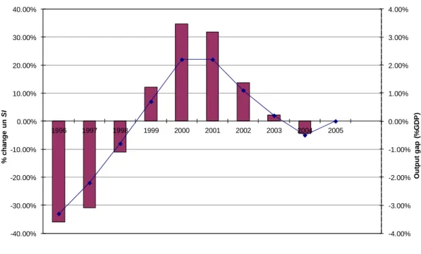
reported. The measure shows a substantial variation over a relatively short period. It starts at 4.11 in 1996 and falls almost monotonically to 2.39 in 1999. From then on it increases again, reaching a maximum value of 4.48 in 2004, and it goes down again in 2005. This extreme variation illustrates the main concern of this paper: the value of the GA sustainability indicators, indeed, appears to be very sensitive to the business cycle. Furthermore, this variation seems to be strongly correlated to the output gap, as it can be estimated through the EC method, as shown in Figure 2.
By contrast, the value of SI once the budget balance is cyclically-adjusted varies
to a lesser extent. For example, the conventional sustainability gap expressed in terms of annual GDP fell by roughly 0.99 percentage points from 1996 to 1997. The cyclical component of the improvement in this period was 0.48 percentage points, or roughly one half of the overall improvement. The balancing property of the cyclically neutral computation also comes through in the second half of the observation window, when the output gap was declining. For example, in the period from 2003 to 2004, conventional GA indicates that the sustainability gap increased by 0.79 percentage points. The cyclical element in this change was 0.51, or roughly two thirds of the annual change. In other words, roughly one third of the worsening in the fiscal sustainability measure was associated to factors unrelated to the business cycle.
Hence, the first conclusion of our analysis is that the cyclical adjustment of the GA indicators matters. In fact, while the standard generational accounts suggests that the fiscal sustainability stance of Spain, if anything, slightly improved during the time period 1996-2005 (overall change in SI -0.36), cyclically neutral GA reveals that
actually the opposite was the case. From 1996 to 2005, the adjustment need in terms of annual GDP increased from 2.63 percent to 3.75 percent, or roughly 42 percent.
Below we will rely on our proposed decomposition method to show how much of the deterioration in the cyclically neutral accounts over time is due to pure policy
effects, and how much due to the other possible effects, namely the debt evaluation and the demographic effects.
b) Decomposition Uncovering Pure Policy Effects
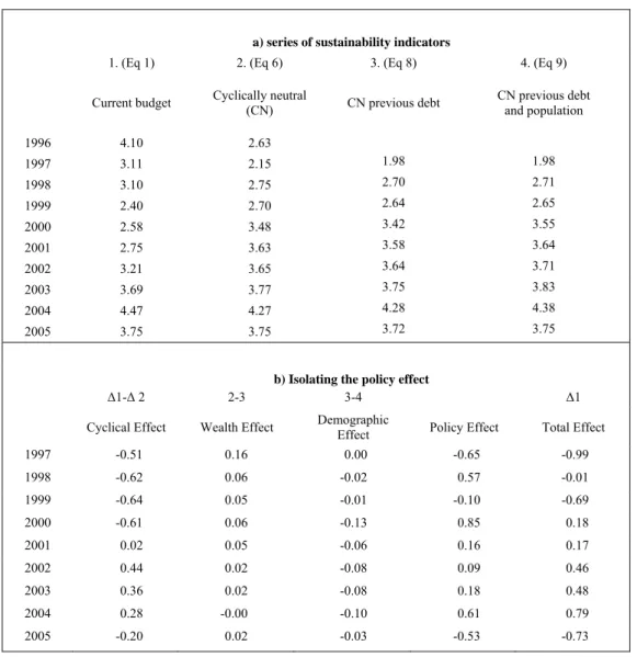
Table 3 shows the complete results for the sustainability indicator SI.7. In the first two
columns of the upper panel a), the value of the sustainability indicator SI is shown
before and after the cycle correction, i.e. estimating equations (1) and (6). The next two columns show the series of sustainability indicators obtained estimating equation (8) – when previous debt is used –, and from equation (9) – with both previous debt and population.
Below, in panel b) the decomposition effect is shown. First, column 1 computes the cycle effect as the difference between the change in sustainability before and after cycle correction. Second, the wealth effect is computed subtracting column 3 from column 2. Third, the demographic effect is calculated as the difference between columns 3 and 4. As indicated above, the policy effect can be obtained as a residual. But it can be also obtained subtracting the sustainability indicator in column 2 for the previous year from column 4, as both are free of cycle effects and contain the same population and wealth figures.
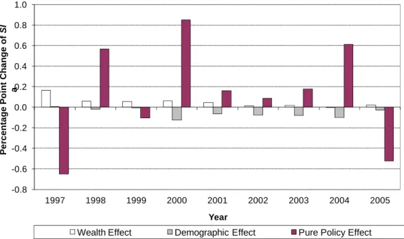
Figure 3 illustrates how the year-to-year changes in the cyclically neutral fiscal sustainability indicator SI decompose into the different effects. With respect to the
wealth effect, we can see that there have been windfall losses worsening sustainability that increase the SI for all periods except for 2004. In most years, this effect if rather
small (below 0.1 percentage points of GDP), and aggregating it over the entire observation window, it is equivalent to 0.43 percent of annual GDP.
Also the demographic effect is rather small throughout, and it has worked in the opposite direction to the wealth effect with the exception of the period 1996-1997. The slight improvement in sustainability for demographic reasons seems to be due to the massive entry of immigrants to Spain during the observation period, which has two opposite effects on fiscal sustainability. On the one hand, the sustainability gap
7 The set of results for the
SG indicator is available from the authors upon request. The results obtained for either of the two indicators are quite similar. Recall that the indicator SI sets the SG in relation to future earnings capacity – the sum of the present value of future GPD. The cycle correction affects both figures in the same direction, i.e., reduces them in an expansion and increases then in a recession, affecting the SI ratio twice, which, consequently, varies to a somewhat greater extent.
becomes larger, as the projected net fiscal contribution of the immigrants is negative. On the other hand, the larger population implies a larger income base to finance the sustainability gap. In other words, the denominator of the SI measure becomes larger, too. The positive demographic effect shows that the latter effect dominates the former.
During the observation window the total of the alleviating demographic effect (-0.49) is almost as large as the additional burden from the wealth effect (0.44). Therefore, the overall development of the cyclically neutral sustainability measure is dominantly a reflection of the pure policy effect we seek to uncover. Figure 3 clearly shows that fiscal policy in Spain, in structural terms, was expansionary during most years of the observation window. The only exceptions are the episodes 1996-97, 1998-99 and 2004-05, when the cyclically neutral sustainability gap declined by 0.65, 0.10 and 0.53 percentage points per annual future GDP, respectively. Policy is shown to worsen in the remainder of the periods, with especially strong structural expansion of future liabilities during 1997-8, 1999-2000 and 2003-4. Therefore, fiscal sustainability in cyclically neutral terms in sum has declined by 1.17 percentage points in terms of annual future GDP.
This contradicts the general perception at that moment of Spain being an outstanding example of fiscal consolidation in the EU.8 In contrast to what conventional generational accounting would tell us, Spain did not manage to consolidate its intertemporal liabilities in the period before the current economic crisis. In fact, one may claim that the current public debt crisis in Spain is to some extent a reflection of insufficient budgetary discipline during the previous decade of above average growth and declining interest payments on public debt, which seemingly improved fiscal sustainability. By looking at Table 2, we can see that positive tendencies in some budget aggregates (e.g., unemployment expenditures, age-related expenditure due to certain pension cuts) are outweighed by growth in non-age-related expenditures. Probably the decentralization process, in which Spain was involved at that time, had a role in this trend.
Nevertheless, if one considers the slight overall improvement in fiscal sustainability associated with the pure cyclical effect, it is also true that things could
8 See Mulas et al.(2004) and González-Páramo (2001) for a discussion on the Spanish fiscal consolidation
have gone even worse if Spain had wasted the improvement in short term fiscal balances during the expansionary phase of the business cycle.
4. Concluding Remarks
Generational accounting has become a broadly applied technique for assessing long-term feasibility of fiscal policies. It is especially well suited to evaluate the effects of demographic ageing on intertemporal fiscal sustainability. One of the drawbacks of the technique, however, is the sensitivity of the resulting sustainability indicators with respect to the business cycle. As a consequence, generational accounting indicators may not be very informative when it comes to comparing intertemporal fiscal imbalances over time or across countries. This is true, even if the underlying empirical standards as regards the demographic and fiscal forecasting procedures are identical.
The paper shows a solution to this issue: a methodological modification of generational accounting, which aims at fiscal sustainability indicators that are independent of the cycle. The method relies on incorporating cyclically-adjusted balances (computed according to established standards) into the forward-looking budget projections underlying the concept.
Our empirical application using data from Spain demonstrates that the differences between conventional and cyclically neutral generational accounting can be very substantial. In our example case the two methods lead to completely different judgements of how fiscal sustainability changed during the window of observation. While conventional generational accounting would suggest a consolidation process (associated with growing primary surpluses), the cyclically neutral approach reveals that in structural terms, the consolidation measures adopted by fiscal policy decision makers actually were inadequate to render fiscal policy truly sustainable even in a neutral macro economic growth environment. Hence, apparently, the need to prepare for the EMU seems to have failed to have the expected effect on fiscal consolidation. Probably, the internal decentralization process in which Spain was involved during the same period, acted in the opposite direction.
From the example application of our proposed method, one should not conclude, however, that measurement error in the pure policy effect when looking at first differences of conventional generational accounting measures is always substantial. In
fact, comparing of our results with previous findings for Germany by Hagist and Benz (2008) suggests that the differences between the conventional and the cyclically neutral fiscal sustainability measures could be much smaller under different circumstances. A key parameter of how important the budget cycle can be in a generational accounting analysis is the degree to which automatic stabilizers smoothing cyclical budget balances are built into the respective fiscal system. In countries where automatic stabilizers play an important role, like in the Germany, the necessity for cyclically neutral approaches will be less strong than in countries where automatic stabilizers are relatively week, like in Spain.
The sensitivity of the gap between conventional and cyclically adjusted fiscal sustainability indicators to the size and structure of automatic stabilizers would warrant attention in further research. Thus, additional country studies of cyclical effect, or a more formal assessment based on systematic numerical simulations of model economies, would be welcome. In any case, cyclically neutral generational accounting measures will remain if one seeks to draw cross-country comparisons: not only the current state of the cycle, but also the role of automatic stabilizers will generally differ between countries.
To conclude, it is worth highlighting that our proposed method does not only take care of cyclical fluctuations. It furthermore allows for handling two additional effects that are independent of the cycle, but may obscure the pure policy effect of interest – a debt evaluation effect and a demographic effect. Again, our practical application shows that these theoretically conceivable effects can also be of practical importance. Therefore, it appears that not only the cycle correction method but also the proposed further decomposition technique of the cyclically neutral sustainability measures is in order, whenever the task is to make generational accounting results comparable over time and/or across countries.
References
Abío, G., E. Berenguer, H. Bonin, J. Gil, and C. Patxot (2005), Contabilidad Generacional en España, Estudios de Hacienda Pública, Instituto de Estudios
Fiscales.
Abío, G.; H. Bonin; E. Berenguer; J. Gil and C. Patxot (2001), “Is the Deficit under Control? A Generational Accounting Perspective on Fiscal Policy and Labour Market Trends in Spain”, Investigaciones Economicas, Vol. 27(2), 309-341.
Auerbach, A.J. (1997), “Quantifying the Current U.S. Fiscal Imbalance”, National Tax Journal, Vol. 50(3): 387-398.
Auerbach, A.J., J. Gokhale and L.J. Kotlikoff (1991), “Generational Accounts: a Meaningful Alternative to Deficit Accounting”, in D. Bradford (ed.), Tax policy and the economy (Vol. 5), Cambridge: MIT Press: 55-110.
Auerbach, A.J., J. Gokhale and L.J. Kotlikoff (1992), “Generational Accounting: A New Approach to Understanding the Effects of Fiscal Policy”, Scandinavian Journal of Economics, Vol. 94(2): 303-318.
Auerbach, A. J; L. Kotlikoff and W. Leibfritz (1999), Generational Accounting around the World, Chicago, University of Chicago Press.
Balassone, F. and D. Franco (2000), “Assessing Fiscal Sustainability: A Review of Methods with a View to EMU”, in: Banca d’Italia, Research Department (ed.),
Fiscal Sustainability: 21-60.
Balassone, F., J. Cunha, G. Langenus, B. Manzke, J. Pavot, D. Prammer and P. Tommasino (2009). Fiscal Sustainability and Policy Implications for the Euro Area. Deutsche Bundesbank Research Centre, Discussion Paper Series 1:
Economics Studies 09/04, Frankfurt.
Blanchard, O., J.C. Chouraqui, R.P. Hagemann and N. Sartor (1990), “The Sustainability of Fiscal Policy: New Answers to an Old Question”, OECD Economic Studies 15: 7-36.
Berenguer, E., B. Raffelhüschen and H. Bonin (1999), “Spain: the Need for a Broader Tax Base”, in European Commission (ed.), Generational accounting in Europe,
European Economy, Reports and Studies, 1999/6, Brussels: 71-85.
Bonin, H., B Raffelhüschen and J. Walliser (2000), “Can Immigration Alleviate the Demographic Burden?”, Finanzarchiv, Vol. 57(1): 1-21.
Bonin, H., J. Gil and C. Patxot (2001), “Beyond the Toledo Agreement: the Intergenerational Impact of Spanish Pension Reform”, Spanish Economic Review, Vol. 3(1): 111-130.
Börstinghaus, V. and G. Hirte (2001): “Generational Accounting versus Computable General Equilibrium”, Finanzarchiv, Vol.58(3): 227-243.
Buiter, W. H. (1997), “Generational Accounts, Aggregate Saving and Intergenerational Redistribution”, Economica, Vol. 64(November), 605-626.
Buti, M. (2002), “Revisiting the Stability and Growth Pact: Grand Design or Internal Adjustment?”, in Seminario: “La Estabilidad Presupuestaria: Crecimiento y Bienestar Social”, Fundación SEPI, Nov. 2002.
Corrales F., J. Varela, R. Doménech (2002): “Los Saldos Presupuestarios Cíclico y Estructural de la Economía Española”, Hacienda Pública Española/Revista de Economía Pública, 162-(3-2003): 9-33
De Castro, F., J. M. González-Páramo and P. Hernández de Cos (2004): “Fiscal Consolidation in Spain: Dynamic Interdependence of Public Spending and Revenues”, Investigaciones Económicas, Vol. 28(1): 193-207.
Diamond, P. A. (1994), “Generational Accounts and Generational Balance: an Assessment”, National Tax Journal, Vol. 49(4): 597-607.
Domar, E. D. (1944), “The Burden of the Debt and the National Income”, American Economic Review, Vol. 34(4): 798-827.
Doménech, R. and D. Taguas (1999), “El Impacto a Largo Plazo de la UEM sobre la Economía Española”, in R. Caminal (ed.), El euro y sus repercusiones sobre la economía española, Fundación BBV: 93-138.
Égert, B. (2010), “Fiscal Policy Reaction to the Cycle in the OECD: Pro- or Counter-cyclical?”, OECD Economics Department Working Papers, No. 763, OECD
Publishing. Paris.
European Commission (1999), Generational Accounting in Europe, European
Economy, Reports and Studies, 1999/6, Brussels.
European Commission (2002): Cyclical Adjustment of Budget Balances. European
Commission Directorate General ECFIN, Economic and Financial Affairs (2002) DG ECFIN Economic Forecast, Last update Spring 2012.
European Commission (2000): Public Finance in the EMU, European Economy No
3/2000, Directorate General Economic and Financial Affairs (ECFIN). Last update 2011.
Fehr, H. and L. Kotlikoff (1996), “Generational Accounting in General Equilibrium”,
Finanzarchiv, Vol. 53(1): 1-27.
Fehr, H. and L. J Kotlikoff (1999), “Generational Accounting in General Equilibrium”, in A. J. Auerbach, L. Kotlikoff and W. Leibfritz (1999), Generational Accounting around the World, Chicago, University of Chicago Press: 43-71.
Feist, K., B. Raffelhüschen, R. Sullström and R.Vanne (1999), “Finland: Macroeconomic Turnabout and Intergenerational Redistribution”, in European Commission (ed.), Generational Accounting in Europe, European Economy,
Reports and Studies 1999/6: 163-178.
FBBV – Fundación Banco Bilbao Vizcaya (1997) Pensiones y Prestaciones por Desempleo, 2ª Edición. Fundación BBV.
Girouard, N. and C. André (2005), Measuring Cyclically-Adjusted Budget Balances for
OECD Countries, OECD Economics Department, Working Papers, No. 434,
OECD Publishing, Paris.
González-Páramo, J.M. (2001), Costes y Beneficios de la Disciplina Fiscal: la Ley de Estabilidad Presupuestaria en Perspectiva, Colección de Estudios de Hacienda
Pública, Instituto de Estudios Fiscales.
Benz, U. and C. Hagist (2008), “Konjunktur und Generationenbilanz - Eine Analyse anhand des HP-Filters”, Journal of Economics and Statistics, Vol. 228(4),
299-316.
Haveman, R. (1994), “Should Generational Accounts Replace Public Budgets and Deficits?”, Journal of Economic Perspectives, Vol. 8(1): 95-111.
Herce, J. A. and J. Alonso (2000), “Los Efectos Económicos de la Ley de Consolidación de la Seguridad Social”, Hacienda Pública Española 152,
1/2000.
IGAE – Intervención General de la Administración del Estado (1998-2005), Cuentas de las Administraciones Públicas.
Larch, M. and A. Turrini (2009), The Cyclically-Adjusted Budget Balance in EU Fiscal Policy Making: A Love at First Sight turned into a Mature Relationship,
European Economy, Economic Papers 374, March 2009.
MTAS – Ministerio de Trabajo y Asuntos Sociales (2001), Anuario de Estadísticas Laborales y de Asuntos Sociales, 2001.
MTSS – Ministerio de Trabajo y Seguridad Social (1995), La Seguridad Social en el Umbral del Siglo XXI: Estudio Económico Actuarial, Madrid.
Mulas, C., J. Onrubia and J. Salinas, J. (2003), “Política Presupuestaria en España (1978-2003)”. In J. Salinas, J. and S. Álvarez. (eds.), El Gasto Público en la Democracia. Estudios en el XXV Aniversario de la Constitución Española de 1978. Instituto de Estudios Fiscales (2003): 383-405.
OECD (2002), “Fiscal Sustainability: The Contribution of Fiscal Rules”, OECD Economic Outlook, 72(December 2002): 117-136.
Patxot, C., E. Rentería, M. Sánchez Romero and G. Souto (2012), “Measuring the Balance of Government Intervention on Forward and Backward Family Transfers using NTA Estimates: The Modified Lee Arrows”, International Tax and Public Finance, Vol. 19(3): 442-461.
Raffelhüschen, B. (1999), Generational Accounting: Data, Method, and Limitations, in
European Commission (ed.), Generational Accounting in Europe, European
Economy, Reports and Studies 1999/6: 17-29.
Raffelhüschen, B. and A. Risa (1997), “Generational Accounting and Intergenerational Welfare", Public Choice, Vol. 93(1/2):149-163.
Van den Noord, P. (2000), The Size and Role of Automatic Fiscal Stabilizers in the
1990s and Beyond, OECD Economics Department Working Papers, No. 230,
OECD Publishing, Paris.
Zubiri, I. (2001), “Las Reformas Fiscales en los Países de la Unión Europea: Causas y Efectos”, Hacienda Pública Española Monografía 2001:13-52.
Figures and Tables
Figure 1. Standard Generational Accounting Sustainability Indicator 1996-2005
Note: Sustainability Gap in Terms of Annual Future GDP. The measure SI indicates the size of the immediate
adjustment of the primary government budget surplus required to achieve fiscal sustainability, in terms of annual GDP.
Figure 2. Correlation of Impact of Cycle Neutralization and Output Gap
0.0 0.5 1.0 1.5 2.0 2.5 3.0 3.5 4.0 4.5 5.0 1996 1997 1998 1999 2000 2001 2002 2003 2004 2005 St a n d a rd SI Year -4.00% -3.00% -2.00% -1.00% 0.00% 1.00% 2.00% 3.00% 4.00% -40.00% -30.00% -20.00% -10.00% 0.00% 10.00% 20.00% 30.00% 40.00% 1996 1997 1998 1999 2000 2001 2002 2003 2004 2005 O u tput ga p (% G D P ) % c h a nge un SI
Figure 3. Decomposition of Annual Changes in Cyclically Neutral Fiscal Sustainability Indicator -0.8 -0.6 -0.4 -0.2 0.0 0.2 0.4 0.6 0.8 1.0 1997 1998 1999 2000 2001 2002 2003 2004 2005 P e rc ent a ge P o in t C h a nge of SI a Year
Table 1 Elasticity of Public Budget Aggregates with Respect to Output Gap
Corporate
Taxes Personal Taxes Indirect Taxes
Social Security Contributions
Current
Expenditure Balance Total Spain 1.15 1.92 1.00 0.68 -0.15 0.44 OECD 1.50 1.26 1.00 0.71 -0.10 0.44 Euro area 1.43 1.48 1.00 0.74 -0.11 0.48
New EU
members 1.38 1.15 1.00 0.71 -0.06 0.42 Source: Girouard and André (2005)
Table 2 Budget Aggregates 1996-2005 (% GDP)
Taxes/Year 1996 1997 1998 1999 2000 2001 2002 2003 2004 2005
VAT 4.9 5.0 5.2 5.7 5.7 5.5 5.6 5.8 6.4 6.4
Personal Income Tax 7.3 7.4 7.2 6.7 6.5 6.6 6.7 6.5 6.4 6.6 Social Security Contributions 12.2 12.2 12.1 12.2 12.0 12.2 12.2 12.2 12.2 12.2 Excise Taxes 2.8 2.9 3.1 3.1 2.8 2.7 2.6 2.5 2.5 2.5 Capital Income Tax and Other Taxes 3.8 3.8 3.8 4.2 4.3 4.0 4.4 4.3 4.6 5.2
Total Age-Specific Revenue 31.0 31.4 31.4 31.9 31.3 31.0 31.3 31.3 31.8 32.7
Transfers
Contributory Pensions 9.9 9.7 9.5 9.3 9.1 8.8 8.7 8.6 8.6 8.5 Non-Contributory Pensions 0.3 0.3 0.3 0.3 0.3 0.3 0.3 0.2 0.2 0.2 Unemployment and Temporary Incapacity 2.8 2.5 2.2 2.0 1.9 2.0 2.1 2.1 2.2 2.1 Health Expenditure 5.5 5.4 5.4 5.4 5.2 5.2 5.2 5.3 5.5 5.7 Family and Long-Term Care 0.8 0.8 0.8 0.8 0.8 0.8 0.8 0.8 0.8 0.8 Educational Expenditure 4.7 4.6 4.6 4.5 4.4 4.3 4.3 4.45 4.4 4.4
Total Age-Specific Expenditure 24.1 23.4 22.9 22.4 21.7 21.4 21.5 21.4 21.8 21.7
Non-Age-Specific Net Expenditure 6.5 6.4 6.8 7.0 7.3 7.1 7.5 7.5 8.1 8.0
Primary Balance 0.4 1.6 1.7 2.5 2.4 2.5 2.4 2.3 1.9 3.0
Interest Payments 5.3 4.9 4.5 3.8 3.5 3.5 3.2 2.9 2.6 1.8
Current Balance -5.0 -3.3 -2.7 -1.3 -1.2 -0.9 -0.8 -0.5 -0.6 1.3
Initial – past year - Debt / GDP 61.0 64.7 63.1 61.2 57.4 55.0 51.9 49.1 45.6 43.2 Output Gap -3.3 -2.2 -0.8 0.7 2.2 2.2 1.1 0.2 -0.5 0.0 Cyclically Adj Primary Balance 1.6 2.3 2.0 2.2 1.6 1.8 2.1 2.3 2.1 3.1
Table 3 Decomposition of Changes in Fiscal Sustainability Indicator (SI)
a) series of sustainability indicators
1. (Eq 1) 2. (Eq 6) 3. (Eq 8) 4. (Eq 9) Current budget Cyclically neutral (CN) CN previous debt CN previous debt and population
1996 4.10 2.63 1997 3.11 2.15 1.98 1.98 1998 3.10 2.75 2.70 2.71 1999 2.40 2.70 2.64 2.65 2000 2.58 3.48 3.42 3.55 2001 2.75 3.63 3.58 3.64 2002 3.21 3.65 3.64 3.71 2003 3.69 3.77 3.75 3.83 2004 4.47 4.27 4.28 4.38 2005 3.75 3.75 3.72 3.75
b) Isolating the policy effect
Δ1-Δ 2 2-3 3-4 Δ1
Cyclical Effect Wealth Effect Demographic Effect Policy Effect Total Effect
1997 -0.51 0.16 0.00 -0.65 -0.99 1998 -0.62 0.06 -0.02 0.57 -0.01 1999 -0.64 0.05 -0.01 -0.10 -0.69 2000 -0.61 0.06 -0.13 0.85 0.18 2001 0.02 0.05 -0.06 0.16 0.17 2002 0.44 0.02 -0.08 0.09 0.46 2003 0.36 0.02 -0.08 0.18 0.48 2004 0.28 -0.00 -0.10 0.61 0.79 2005 -0.20 0.02 -0.03 -0.53 -0.73