X
INTRODUCTION
Inventory means any stored resource that is used to satisfy a current or a future need; for example, the raw materials and finished goods. Therefore the inventory control is crucial for every company. Reducing on-hand inventory level means reducing costs and thus increases the cash flow. On the other hand frequent stock-outs may dissatisfy the customers. Thus a company must make a balance between low and high inventory levels. The major factor to be considered in achieving this balance is the cost minimisation.
T
T
o
o
p
p
i
i
c
c
7
7
X
Deterministic
Inventory
Models
LEARNING OUTCOMES
By the end of this topic, you should be able to: 1. Explain the importance of inventory control;
2. Compute the EOQ and EPQ to determine how much to order or produce;
3. Compute the ROP in determining when to order; and 4. Solve inventory problems that allow quantity discounts.
INVENTORY DECISIONS
There are two fundamental decisions that we have to make when controlling inventory:
1. How much to order or produce? 2. When to order?
The major objective in controlling inventory is to minimize the total inventory costs which include:
1. Cost of the items (purchase cost or material cost), 2. Cost of ordering,
3. Cost of carrying or holding inventory and 4. Cost of stock outs.
ECONOMIC ORDER QUANTITY (EOQ)
This is the basic model in achieving an optimal ordering quantity which minimises the total inventory costs. However there are some assumptions to be upheld:
(a) Demand is known and constant.
(b) The lead time, the time between the placement of order and the receipt of the order, is known and constant.
(c) The receipt of inventory is instantaneous. (d) Quantity discounts are not possible.
(e) The only variable costs are the ordering cost and the holding or carrying cost.
(f) Orders are placed so that stock outs or shortages are avoided completely.
7.2
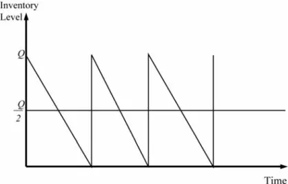
These assumptions lead to an inventory usage of a saw tooth shape, as shown in Figure 7.1.
Figure 7.1: Inventory usage over time in a simple model
7.2.1 Inventory Costs in the EOQ Situation
Let Q be the amount ordered. Thus an inventory levels increases from 0 to Q units when an order arrives. Since the inventory level changes daily, we use the average inventory level to determine the annual holding or carrying cost.
Therefore,
Maximum inventory level = Q Average inventory level =
2 Q
The following variables are important in developing mathematical expressions for the annual ordering and carrying costs.
Ordering quantity = Q
EOQ = Q*
Annual Demand = D Ordering cost per order = Co Holding or carrying cost per unit per year = Ch
Annual Ordering Cost = (number of orders per year) × (ordering cost per order) = Q D u Co = Co Q D
Annual Holding Cost = (average inventory) × (carrying cost per unit per order) = 2 Q uCh = QCh 2
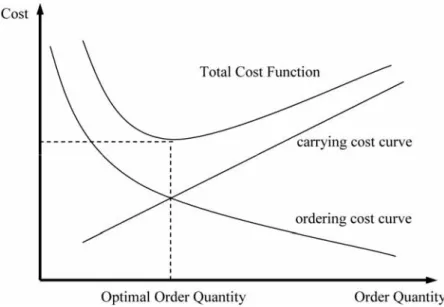
Figure 7.2 shows the graph of the ordering cost, holding cost and the total inventory cost. The lowest point on the total cost occurs where the ordering cost is equal to the holding cost.
7.2.2 Finding the EOQ
The above graph shows that the total costs are minimised when Annual Ordering Cost = Annual Holding Cost
o C Q D = QCh 2 2 Q = h o C DC 2 Q = h o C DC 2
In some context, the holding or carrying cost is expressed as a percentage of the unit cost, I.
Therefore the holding cost will be calculated as: h
C = IC
where C = cost per unit.
7.2.3 Finding the ROP (Re-Order Point)
The second inventory question is ‘when to order’. For this, we should know the lead time first. Lead time, L, (or delivery time) means the time between the placing and receipt of an order. This could be few days or few weeks and inventory must meet the demand during these days. Therefore,
ROP = (demand per day) × (lead time) = d × L
This means, an order is placed when the inventory level reaches the ROP, and the new inventory arrives at the same instant the inventory is reaching 0.
7.2.4 Economic Order Quantity (EOQ) Model
Annual Ordering Cost = CoAnnual Holding Cost = Ch
EOQ = Q* = h o C DC 2
Total Annual Inventory Cost
(including purchasing cost) = QCo D
+QCh 2 + DC Re Order Point, ROP = d u L
Example 7.1
A Hardware Shop in Subang Jaya sells 2,500 brackets in a year and the sales is relatively constant throughout the year. These brackets are purchased from a supplier from Ipoh for RM15.00 each, and the lead time is two days. The holding cost per bracket per year is RM1.50 (or 10% of the unit cost) and the ordering cost per order is RM18.75. There are 250 working days per year.
1. What is the EOQ?
2. Given the EOQ, what is the average inventory? What is the annual inventory cost?
3. In minimising the cost, how many orders would be made each year? What would be the annual ordering cost.
4. Given the EOQ, what is the total annual inventory cost (including purchase cost)?
5. What is the time between orders? 6. What is the ROP?
Solution:
Annual Demand, D = 2500
Ordering cost per order, Co = RM18.75 Holding or carrying cost per unit per year, Ch = RM150 and I = 0.10
Unit cost, C = RM15.00
Lead time, L = 2 days
Number of working days, Wd = 250 days
1. EOQ = Q* = h o C DC 2 = 2 2500 18.75 1.50 u u = 250 brackets 2. Average inventory = 125 2 250 2 Q
Annual inventory cost = 250(1.50) RM187.50 2 h 2
Q C
3. # of orders per year = 10 250 2500 Q
D
Annual ordering cost = 2500(18.75) RM187.50 250
o D
C Q
4. Total Annual Inventory Cost
(including purchasing cost) = Q Co D
+QCh 2 + DC
= 187.50 + 187.50 + (2500 u 15)
= RM 37875
5. Time between orders = Wd per year 250 25 days # orders per year 10
6. ROP daily demand lead time 2500 2 100 2 200 brackets 250
ECONOMIC PRODUCTION QUANTITY (EPQ)
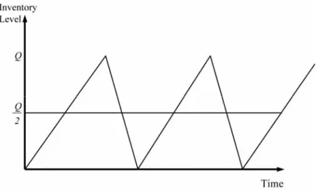
In the production environment, the inventory continuously flows or builds up over a period of time after an order has been placed or when units are produced and sold simultaneously. Hence, the daily demand rate must be taken into account in this model. Figure 7.3, shows the inventory levels as a function of time.Figure 7.3: Inventory usage over the time in a production run model
In this model, we have setup cost, Cs i.e. cost of setting up the production facility
to manufacture the desired product. The holding cost per unit per year, remains unchanged. However the annual holding cost changes due to the change in average inventory level.
The following variables are used in developing mathematical expressions for the annual setup and carrying costs for a production run model:
Production Quantity = Q
EPQ = Q*
Annual Demand = D Setup Cost per production run = Cs Holding or carrying cost per unit per year = Ch Daily production rate = p
Daily demand rate = d Length of production run in days = t
7.3
7.3.1 Inventory Costs in the EPQ Situation
Maximum inventory level = (total production in t days) – (total demand in t days)
= ptdt
= t p d
As the production quantity is Q where Q = pt which gives t = Q. p Maximum inventory level = ptdt
= t p d
= Qp d p = 1Q d p § · ¨ ¸ © ¹ Average Inventory = 1 2 Q d p § · ¨ ¸ © ¹Annual Holding Cost = (average inventory) × (carrying cost per unit per order) = 1 2 h Q d C p § ·u ¨ ¸ © ¹ = 1 2 h Q d C p § · ¨ ¸ © ¹
Annual Setup Cost = (number of production per year) × (setup cost per order) = Q D u Cs = Cs Q D
7.3.2 Finding the EPQ
The total inventory costs are minimised when Annual Setup Cost = Annual Holding Cost
s C Q D = 1 2 h Q d C p § · ¨ ¸ © ¹ 2 Q = 2 1 s h DC d C p § · ¨ ¸ © ¹ Q = 2 1 s h DC d C p § · ¨ ¸ © ¹
7.3.3 Economic Production Quantity (EPQ) Model
Annual Setup Cost = CsQ D
Annual Holding Cost = Ch p d Q ) 1 ( 2 EPQ = Q* = h s C p d DC ) 1 ( 2
Total Annual Inventory Cost
(including purchasing cost) = QCs D + Ch p d Q ) 1 ( 2 + DC Re Order Point, ROP = d u L
Example 7.2
The Hardware Shop in Subang Jaya (refer the Example 7.1), wants to reconsider its decision of buying the brackets and is considering in-house, production. The setup cost would be RM25.00 and 50 brackets could be produced in a day once the machine has been setup. The cost of producing one bracket is estimated as RM14.80. The holding cost would be 10% of this cost.
1. What is the daily demand rate? 2. What is the EPQ?
3. How long will it take to produce the optimal production quantity? How much inventory is being sold during this time?
4. Given the EPQ, what is the maximum inventory level? What is the average inventory? What is the annual inventory cost?
5. In minimising the cost, how many production runs would there be each year? What would be the annual setup cost?
6. Given the EPQ, what is the total annual inventory cost (including production cost)?
7. If the lead time is one and a half-day, what is the ROP? Solution:
Annual Demand, D = 2500
Daily production rate, p = 50
Setup cost per order, Cs = RM25.00 Holding or carrying cost per unit per year, Ch = RM1.48 and I = 0.10
Unit cost, C = RM14.80
Lead time, L = 0.5 day
1. Demand rate, d = annual demand 2500 10 # of working days 250 2. EPQ = Q* = h s C p d DC ) 1 ( 2 = 2 2500 25 10 1 1.48 50 u u § · ¨ ¸ © ¹ = 325 brackets
3. Production time, t = Production Qty 325 6.5 days Production rate 50
Inventory sold during t days = t u d = 6.5u 10 = 65 brackets 4. Maximum inventory = production – inventory sold = 325 – 65 = 260
Average inventory = Max inventory 260 130
2 2 or Average inventory = 1 325 1 10 130 2 2 50 Q d p § · § · ¨ ¸ ¨© ¸¹ © ¹
Annual inventory cost = 1 325 1 10
1.48 RM192.402 h 2 50 Q d C p § · § · ¨ ¸ ¨© ¸¹ © ¹
5. # of production run per year = 2500 7.7 runs 325
D Q
Annual setup cost = 2500 25 RM192.30 325
s D
C Q
6. Total Annual Inventory Cost
(including purchasing cost) = QCs D + Ch p d Q ) 1 ( 2 + DC = 192.30 + 192.40 + (2500 u 14.80) = RM37384.70
7. ROP daily demand lead time 2500 0.5 10 0.5 5 brackets 250
u u u
Comparing both the example 7.1 and 7.7, the in-house production is cheaper.
QUANTITY DISCOUNT MODEL
The deterministic inventory control models, previously considered have been developed under the assumption that the unit cost of an item was independent of the quantity produced or ordered. However, in many business and industries, quantity discounts are provided as incentives for the purchase of larger quantities of products. When quantity discounts are available and all the EOQ assumptions are met, it is possible for us to find the quantity that minimises the total annual inventory cost (or simply said, the total cost). As the discounts are usually lowering the material cost or the unit cost of a product, based on the order quantity, we have to calculate the total cost based upon the order quantity in determining the optimal ordering quantity.
Total Cost = material cost + ordering cost + carrying cost
= Co Q D + QCh 2 + DC or = Cs Q D + 1 2 h Q d C p § · ¨ ¸ © ¹ + DC
The process for determining the minimum total cost as follows: 1. For each discount price (C), compute the EOQ,
Q* = h o C DC 2 or 2 1 s h DC d C p § · ¨ ¸ © ¹
2. If Q* < minimum for discount, adjust the quantity to Q = minimum for discount.
3. For each Q* or adjustedQ, compute the total cost.
7.4
4. Check for the lowest total cost and select that option for optimal ordering quantity.
Example 7.3
A company that produces aluminium foil, offers the following discount schedule for its 4’ u 4’ sheets:
Discount Category Order Size Discount (5%) Unit Cost (RM)
A 0 to 1499 0 10.00
B 1500 to 2499 2 9.80
C More than 2500 5 9.50
Saro Mini Market orders aluminium foils from the company above. The mini market’s ordering cost is RM100. The carrying cost is 20% of the unit cost and the annual demand is 2000 sheets. What do you recommend?
Solution:
D = 2000, Co= RM100, I = 0.2.
Discount
Category Order Size
Unit Cost (RM) EBQ = Q* = 2DCo IC Adjusted Ordering Quantity, Q Total Cost 2 o DC QIC + DC Q A 0 to 1499 10.00 447 447 20894.43 B 1500 to 2499 9.80 452 1500 21203.33 C More than 2500 9.50 459 2500 Exceeded D
Comparing the discount options of A, B and C, we find that option A, without discount, reduces the annual inventory cost. Therefore its better to keep the ordering quantity at 447 sheets.
ABC
ANALYSIS
A company’s inventory is divided into three groups i.e. Group A, Group B and Group C based on the overall inventory value. In another word, ABC categorises inventory by its highest value and greatest volume. Managing the greatest value of inventory is crucial as it saves a lot for the company. But this may consist only about 5–15% of the inventory. The table below mentions a brief description of each group with general guidelines as how to categorise them.
Inventory Group Inventory Value (%) Inventory (%) Importance of Inventory Management A 70–80 5–15 Yes B 15 30 Moderate C 5–10 50–60 No
Segmentation may not always occur so neatly. The objective, though, is to try to separate the important from the unimportant. Where the line actually breaks depends on the particular inventory under question and on how much personnel time is available.
Figure 7.4: Percentage of total list of different stock items
7.5.1 Steps to ABC Analysis
(a) Sort products from largest to smallest annual $ volume.
(b) Divide into A, B and C classes.
(c) Focus on A products.
(i) Develop class A suppliers more.
(ii) Give tighter physical control of A items.
(iii) Forecast A items more carefully.
(iv) Consider B products only after A products. Example 7.4
The following table describes a company’s inventory items with unit cost and annual usage. Illustrate using an ABC plan.
Part Unit Cost Annual Usage
1 2 3 4 5 6 7 8 9 10 $60 350 30 80 30 20 10 320 510 20 90 40 130 60 100 180 170 50 60 120 Part Total Value % of Total Value % of Total Quantity % Cummulative 9 $30,600 35.9 6.0 A 6.0 8 16,000 18.7 5.0 11.0 2 14,000 16.4 4.0 15.0 1 5,400 6.3 9.0 B 24.0 4 4,800 5.6 6.0 30.0 3 3,900 4.6 10.0 40.0 6 3,600 4.2 18.0 58.0 5 3,000 3.5 13.0 C 71.0 10 2,400 2.8 12.0 83.0 7 1,700 2.0 17.0 100.0 $85,400
1. In a supermarket, an electrical product costs RM1,000, the annual holding cost is 25% and the annual demand is 10,000 units. The ordering cost per order is RM150. What is the ordering size to minimise the inventory costs?
(Answer: 70) 2. In a basic EPQ model, the daily production rate is 25 units. Given that the annual demand is 6000 units, setup cost,Cs= RM100 and annual holding cost, Ch= RM5, find the optimal production quantity.(Assume the annual working days is 300).
(Answer: 1732) 3. In an electrical shop, the cost-minimising order quantity obtained with the basic EOQ model for an electrical item was 200 units and the total annual inventory cost was RM600. What is the inventory carrying cost per unit per year for this item?
(Answer: RM3.00) 4. Demand for a certain product ordered by a mini market tends to be constant at a monthly rate of 1000 units. Annual holding cost for this item is RM5.00 per unit and the cost of placing an order is RM20.00. (a) Find the optimal order size and how often this order should
be placed?
(b) What is the relevant total inventory cost, excluding the purchasing cost?
(c) If the mini market makes orders every week, what is the percentage increase in the relevant total inventory cost? (d) Suppose this product can be ordered in multiples of
100 units, what is the best order size?
(Answer: (a) 310 units, every 9 days (c) 8%)
5. (a) KH textile sells 175 pieces of hand towels per month. The unit cost of a towel is RM2.50 and the cost of placing an order has been estimated at RM12.00. The store uses an inventory carrying charge of 27% per year. Find the optimal order quantity, order frequency, and the total annual inventory cost.
(Answer: 273 units, 8 orders, RM184.44) (b) If the order is placed online, the ordering cost shall decrease to RM4.00. What would be the new economic order quantity, order frequency, and the total annual inventory cost? Explain these results.
(158 units, 13 orders, RM106.48) 6. The annual demand for an item is 1000 units. The cost to process an order is RM50.00 and the annual inventory holding cost is 25% of the unit cost per item per year. The unit cost per item is RM50.What is the optimal ordering quantity, given the following quantity discount schedule?
Order size Discount(%)
0 to 99 0
100 to 249 3
more than 250 5
(Answer: 250, RM49, 184.00) 7. Muthu Plumbers has a demand for 1000 pumps every year. A
pump costs RM50.00 and the cost to place an order is RM40.00. Annual holding cost per pump is 25% of the unit cost. If the pumps are ordered in quantities of 200, Muthu Plumbers can get a discount of 3% on the unit cost of the pumps. Should Muthu order the pumps in the quantities of 200?
8. The annual demand for a certain electronic product is 6750 units. An electronic company in Port Klang manufactures this product and its daily production capacity is 125 units. The daily demand during the production process is 30 units. If the setup cost is RM150.00 and the carrying cost is RM1.00 per unit per year, what is the optimal production quantity that minimises the annual inventory cost?
(Answer: 1632 units) 9. A refrigerator plant in Bangi has a constant demand of 8000 units a year. The plant can produce 200 units per day and every production run takes a setup cost of RM120.00. The holding cost for refrigerator is RM20.00 per year. Currently the plant produces 400 units in each production and the plant operates 250 days in a year.
(a) What is the daily demand for this product? (b) What is the production time for 400 units?
(c) Under the current policy, what would be the annual setup cost?
(d) Under the current policy, what is the annual holding cost? (e) Under the current policy, what is the total of annual setup
cost and holding cost?
10. Referring to question 8 above, what would be the optimal production quantity minimising the total annual setup and holding cost? How much would this save the plant in the annual inventory cost compared with the current policy?
In this topic we have covered the following:
x The importance of inventory management.
x Compute the EOQ and EPQ to determine how much to order or produce.
x Compute the ROP in determining when to order.
x Handle inventory problems that allow quantity discounts.
x The ABC analysis of inventory management.
Render, B. et al. (2001). Quantitative analysis for management (9th ed.). NJ: Prentice Hall.
Taha, H. A. (2003). Operations research – An introduction. New Jersey: Prentice-Hall.
Hillier, F. S., & Lieberman, G. J. (1990). Introduction to operations research. Singapore; Mc-Graw Hill.