ASAE DISTINGUISHED LECTURE SERIES
Tractor Design No. 27
Traction and Tractor
Performance
Frank M. Zoz and Robert D. Grisso
These lectures have been developed to provide
in-depth resource information for engineers
Copyright © 2003 by the American Society of Agricultural Engineers
All Rights Reserved
Manufactured in the United States of America
This lecture may not be reproduced in whole or in part by any means
(with the exception of short quotes for the purpose of review)
without the permission of the publisher
For information, contact:
ASAE, 2950 Niles Rd., St. Joseph, MI 49085-9659 USA.
Phone: 269 429 0300 Fax: 269 429 3852 www.asae.org
ASAE Publication Number 913C0403
The American Society of Agricultural Engineers is not responsible for statements
and opinions advanced in its meetings or printed in its publications.
They represent the views of the individual to whom they are credited
and are not binding on the Society as a whole.
Traction and Tractor
Performance
Frank M. Zoz
Retired
John Deere Product Engineering Center
Waterloo, Iowa, USA
Robert D. Grisso
Professor
Virginia Tech
Blacksburg, Virginia, USA
For presentation at the 2003 Agricultural Equipment Technology Conference
Louisville, Kentucky, USA
9-11 February 2003
Published by
ASAE – the Society for engineering in agricultural, food, and biological systems
2950 Niles Road, St. Joseph, MI 49085-9659 USA
The Lecture Series has been developed by the Power and Machinery Division Tractor
Committee (PM-47) of ASAE to provide in-depth design resource information for
engineers in the agricultural industry. Topics shall be related to the power plant, power
train, hydraulic system, and chassis components such as operator environment, tires, and
electrical equipment for agricultural or industrial tractors or self-propelled agricultural
equipment.
Table of Contents
INTRODUCTION
...5
TRACTION MECHANICS
...5
Solid Wheel on a Hard Surface
...5
Soft Wheel on a Hard Surface
...6
Deformable Wheel on a Soft Surface
...7
Belt Drives
...8
TRACTION PARAMETERS
...9
Travel Reduction Ratio (TRR)
...9
Net Traction Ratio (NTR)
...10
Tractive Efficiency (TE
) ...11
Gross Traction Ratio (GTR)
...11
Motion Resistance Ratio (MRR)
...11
TRACTION DATA ANALYSIS
...12
Pull Slip and NTR Slip
...12
Tractive Efficiency
...14
Regression Analysis
...17
TRACTION TESTING
...19
Single -Wheel Testing
...20
Using Tractors to Test Tires
...21
Speed Effects
...23
TRACTION PERFORMANCE
...24
Effects of Soil
...24
Effects of Tire Pressure
...25
Effects of Tire Size
...25
Effects of Load on Tire
...26
Belt and Tire Comparisons
...26
SOIL, TIRE, AND TRACTION EQUATIONS
...30
TRACTOR PERFORMANCE
...33
Tractor Performance Spreadsheet
...35
Estimated Drawbar Power
...38
OPTIMIZING TRACTOR DRAWBAR PERFORMANCE
...39
Tires
...39
Ballasting
...39
Ballasting Sensitivity
...43
Ballasting Limitations
...44
Ballast Optimization in the Tractor Performance Spreadsheet
...44
CONCLUSIONS
...45
ACKNOWLEDGEMENTS
...45
Traction and Tractor Performance
Frank M. Zoz, P.E.
Retired, John Deere Product Engineering Center, Waterloo, Iowa Robert D. Grisso, P.E.
Professor, Biological Systems Engineering, Virginia Tech, Blacksburg, Virginia
The primary purpose of agricultural tractors, especially those in the middle to high power ranges, is to perform drawbar work. The value of a tractor is measured by the amount of work accomplished relative to the cost incurred in getting the work done. Drawbar work is defined by pull and travel speed. Therefore, the ideal tractor converts all the energy from the fuel into useful work at the drawbar. In practice, most of the potential energy is lost in the conversion of chemical energy to mechanical energy, along with losses from the engine through the drivetrain and finally through the tractive device. Research shows that about 20% to 55% of the available tractor energy is wasted at the tractive device/soil interface. This energy wears the tires and compacts the soil to a degree that may cause detrimental crop production (Burt et al., 1982).
Efficient operation of farm tractors includes: (1) maximizing the fuel efficiency of the engine and drivetrain, (2) maximizing the tractive advantage of the traction devices, and (3) selecting an optimum travel speed for a given tractor-implement system.
Throughout the years, official tractor performance drawbar tests have been conducted on hard surfaces and in recent years (30+ years) on concrete. While this provides a valid comparison between tractors, the data does not provide much information about performance under field conditions. The primary difference between official tests and field conditions is the performance of the tires or other tractive devices.
The understanding and prediction of tractor performance has been a major goal of many researchers. Tractor performance is influenced by traction elements, soil conditions, implement type, and tractor configuration (Brixius, 1987). It is necessary to understand traction performance to predict tractor performance in the field. Traction equations provide a basis for predicting tractor performance when combined with basic information from official tractor tests.
Computer models allow researchers and designers to investigate many problems related to tractor performance under a wide range of conditions with the goal to improve tractor design, to optimize tractor operational parameters, and to improve the tractor/implement match. Relative importance of these factors affecting field performance of a tractor can be achieved without expensive field-testing. For teachers, models enhance the student's ability to comprehend and compare various parameters that influence tractor performance. These models can also assist tractor operators to improve (fine-tune) and optimize their tractors' setup to match operating conditions.
1. Traction Mechanics
Solid Wheel on a Hard Surface
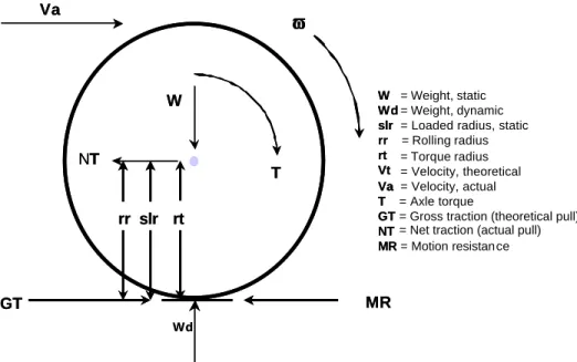
An understanding of traction mechanics is fundamental to understanding differences between tractive performance and tractor performance. The basic forces involved in a powered wheel are shown in figure 1 for the simple case of a solid wheel on a hard surface. The torque input (T) develops a gross traction (GT) acting at the contact surface. Part of the gross traction is required to overcome motion resistance (MR), which is the resistance to the motion of the wheel, including internal and external forces. The remainder is equal to the net traction (NT) that the wheel develops, given by NT = GT - MR.
GT MR slr rr NT T W Va Wd rt ϖ ϖ W = Weight, static Wd= Weight, dynamic
slr = Loaded radius, static
rr = Rolling radius rt = Torque radius Vt = Velocity, theoretical Va = Velocity, actual T = Axle torque GT NT MR GT MR slr rr NT T W Va Wd rt ϖ ϖ W Wd slr rr rt Vt Va T
GT= Gross traction (theoretical pull)
NT= Net traction (actual pull)
MR= Motion resistan ce
Figure 1. Basic wheel forces for a solid wheel on a hard surface.
Soft Wheel on a Hard Surface
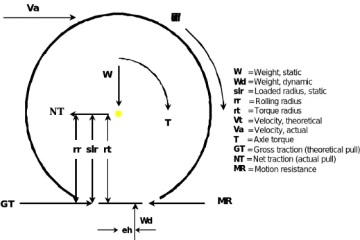
A soft wheel on a hard surface (fig. 2) is much the same as a solid wheel except that it becomes more obvious that the vertical reaction force (Wd) is not directly under the axle centerline but is offset by a distance designated "eh." This offset is necessary for static equilibrium. The amount of the offset is a function of the motion resistance and is given by:
( )( )
W dM R slr
eh = (1)
Three radii are shown in figures 1 and 2: "slr" is the static loaded radius, defined as the distance from the axle centerline to a hard surface; "rr" is the rolling radius, used for speed calculations. Rolling radius is derived from the rolling circumference (usually measured prior to a test but also included in tire
manufacturer data tables). Static loaded radius and rolling radius are close but not equal. For a properly inflated agricultural tire, the rolling radius is about 6% greater than the static loaded radius. Rolling radius should be used for speed calculations. Static loaded radius is more appropriate to use for force or moment calculations. Both can be affected by the softness of the soil surface and are usually determined on a hard surface.
The third radius shown in figure 1 is called the torque radius (rt). This is the effective radius where the gross traction (GT) and motion resistance (MR) forces act. It cannot be measured directly but can be determined by back calculating using energy calculations. This is explained in detail in section 2 of this paper under "Gross Traction Ratio."
MR slr rr NT T W Va Wd GT eh rt ϖ ϖ W = Weight, static Wd= Weight, dynamic
slr = Loaded radius, static
rr = Rolling radius
rt = Torque radius
Vt = Velocity, theoretical
Va = Velocity, actual
T = Axle torque
GT= Gross traction (theoretical pull)
NT= Net traction (actual pull)
MR= Motion resistance MR slr rr NT T W Va Wd GT eh rt ϖ ϖ W Wd slr rr rt Vt Va T GT NT MR
Figure 2. Basic wheel forces for a soft wheel on a hard surface.
Deformable Wheel on a Soft Surface
In the real world, both the wheel and the (soil) surface are deformable and result in the forces and moments shown in figure 3. The result is both a vertical and a horizontal offset, designated "ev" and "eh," respectively. The amount of the offsets depends on the motion resistance force (MR), the tire loaded radius (slr), and the vertical force resultant (Wd):
(
)( )
W d M R ev -slr eh = (2) slr rr NT T W Va GT Wd eh MR ev Ground Line Ground Line rt ϖ ϖ W = Weight, static Wd= Weight, dynamicslr = Loaded radius, static
rr = Rolling radius
rt = Torque radius
Vt = Velocity, theoretical
Va = Velocity, actual
T = Axle torque
GT= Gross traction (theoretical pull)
NT= Net traction (actual pull)
MR= Motion resistance slr rr NT T W Va GT Wd eh MR ev Ground Line Ground Line rt ϖ ϖ W Wd slr rr rt Vt Va T GT NT MR
Belt Drives
The mechanics of the belt drive mechanism (fig. 4) is similar to the wheel in many respects; but the distribution of the load is dependent on vehicle parameters. The location of the dynamic load resultant, "eh" (dynamic balance ratio; Corcoran and Gove, 1985), depends on the static distribution, the design of the suspension mechanism supporting the bogie wheels, and vehicle weight transfer characteristics.
MR slr rr NT T W1 Va Wd GT W2 W3 W4 W5 Ground Line Dh rt ϖ ϖ Vt = Velocity, theoretical Va = Velocity, actual T = Axle torque
GT= Gross traction (theoretical pull)
NT= Net traction (actual pull)
MR= Motion resistance
W = Weight, static
Wd= Weight, dynamic
slr = Loaded radius, static
rr = Rolling radius rt = Torque radius Vt Va T GT NT MR W Wd slr rr rt eh
Figure 4. Belt drive.
In general, the best tractive performance and the most uniform ground pressure on a belt drive can be obtained with a dynamic balance ratio of near 50%. Corcoran and Gove (1985) defined dynamic balance ratio as the ratio of the location of the vertical component of the dynamic load (external loads and tractor weight) from the front of the track divided by the track base length. Unlike a tire, where only the total dynamic weight (Wd) must be considered during a traction test, the dynamic balance of a track mechanism must be considered either in a belt test or a full vehicle test. The dynamic balance ratio obtained depends not only on tractor dimensional parameters and the location and angle of the line of draft but also on the magnitude of the drawbar pull.
Figure 5 shows the effect of draft angle and vehicle traction ratio on the dynamic balance for a tractor with 60% of the static weight at the front. A generic wheel/belt tractor is shown for simplicity, but the weight transfer mechanics are the same for belted and wheel tractors. Note that it only takes a 5° draft angle to give a 50% dynamic balance ratio at a typical vehicle traction ratio of 0.40. Figure 5 is for implements hitched to the drawbar. Even higher weight transfer, and hence higher front weight requirements, may result from the use of three-point hitch equipment.
5 0 10 20 40 42 44 46 48 50 52 54 56 58 60 0 0.1 0.2 0.3 0.4 0.5 0.6
Vehicle Traction Ratio
Dynamic Balance (% Front)
Draft Angle With Dh/Wb= 0.20 Dl/Wb= 0.30 Wb Dl Draft Angle Dh 0.60 0.58 0.56 0.54 0.52 0.50 0.48 0.46 0.44 0.42 0.40
Dynamic Balance Ratio
5 0 10 20 40 42 44 46 48 50 52 54 56 58 60 0 0.1 0.2 0.3 0.4 0.5 0.6 With Dh/Wb= 0.20 Dl/Wb= 0.30 Wb Dl Draft Angle Dh 0.60 0.58 0.56 0.54 0.52 0.50 0.48 0.46 0.44 0.42 0.40
Figure 5. Tractor/belt drive dynamic weight distribution (when starting with 60% static front weight).
2. Traction Parameters
Five dimensionless parameters are used to describe tractive performance:
• Travel reduction ratio (TRR), commonly called "slip" and expressed in percent. • Net traction ratio (NTR), sometimes called pull/weight ratio.
• Tractive efficiency (TE), usually thought of as percent but used as a ratio in this paper. • Gross traction ratio (GTR).
• Motion resistance ratio (MRR).
The traction parameters involving forces are all normalized by dividing by Wd, the dynamic force reaction supporting the wheel or traction device. Wd includes static axle weight and any weight transfer that might take place during the testing process, i.e., the total reaction force. Dividing by Wd allows comparisons between tires and other tractive devices of different sizes and weights, and provides a dimensionless parameter for traction comparisons.
Note that all the traction parameters are normally presented as ratios except travel reduction and tractive efficiency, which are commonly expressed as percentages. Working with traction data is easier if all parameters are presented as ratios. It will become more obvious later, but remember that the above parameters apply to a traction device and not necessarily to a vehicle.
Travel Reduction Ratio (TRR)
Vt Va 1 Velocity l Theoretica Velocity Actual 1 TRR= − = − (3)
Travel reduction has traditionally been called "slip" or "% slip," but technically this is incorrect. Slip occurs between surfaces. Travel reduction is a reduction in distance traveled and/or speed that occurs because of:
• Slip between the surfaces (rubber and concrete, for example) • Shear within the soil.
From a power efficiency standpoint, travel reduction is a power loss caused by a loss in travel speed or distance traveled. Slip (travel reduction) occurs any time a wheel or traction device develops pull (net traction) (Brixius and Wismer, 1978).
Zero travel reduction can be defined using any of four methods (ASAE Standards, 2001b):
1. A self-propelled (zero net traction) condition on a non-deforming surface (recommended for rolling circumference data, as in published tire data).
2. A self-propelled (zero net traction) condition on the test surface.
3. A towed (zero gross traction, i.e., zero torque) condition on a non-deforming surface. 4. A towed (zero gross traction) condition on the test surface.
There are arguments for using any of the above methods for a particular traction test. In any case, the zero condition used to define the rolling radius should always be stated. The most common zero condition is use of the self-propelled condition on the test surface (method 2). However, tire data are usually given for a non-deforming surface (method 1). The difference in measured rolling radii between a non-deforming (hard) surface and a test surface is small under normal agricultural soil conditions (dry and/or untilled soil) and thus makes little difference in the final results. In any case, errors of defining "zero slip" do not affect the final tractive efficiency results, as travel reduction does not enter directly into the equation. It only affects the results where the losses are assigned, that is, either to travel reduction or motion resistance. This will be discussed in more detail in section 3 of this paper.
The authors' preference is to use a self-propelled condition (zero net traction) on a hard surface, and this method is used throughout this paper. This method provides a repeatable test condition, results that should agree closely to published tire data, and data that can be replicated at other locatio ns and test conditions. It is also easy to imagine a case of very soft soil where the zero condition may result in an apparent 100% slip, i.e., the vehicle gets stuck, while being assigned zero travel reduction.
The rolling radius (rr) measured under one of the above methods is used to calculate the theoretical speed (Vt) of the wheel or tractive device:
Vt (m/s) =
ϖ
(rpm) × rr × 2π/60 (4)The actual forward velocity (Va) of the vehicle or wheel is usually measured directly using a fifth wheel or radar device. Both Vt and Va must use the same units of measurement.
Net Traction Ratio (NTR)
W d NT Force Reaction Dynamic Traction Net NTR= = (5)
The net traction ratio is sometimes referred to as pull/weight, P/W, dynamic traction ratio, or coefficient of traction. Most of these terms actually refer to a complete vehicle rather than to a simple traction device. The dynamic reaction force or dynamic weight (Wd) includes the effects of ballast and any weight transfer that may occur in the testing process. If a complete vehicle is used for the traction device testing, the weight may include front to rear transfer due to horizontal pull, and any transfer due to implement or load unit draft angle. The net traction force (NT) must be the force component in the direction of travel and perpendicular to the reaction force (Wd).
As stated, the above equation applies to a tractive device and not to a comp lete vehicle. For a total vehicle (tractor), the equivalent to net traction ratio (NTR) is vehicle traction ratio (VTR), which is the vehicles' drawbar pull divided by the total vehicle dynamic weight. This will be covered in more detail in section 7 of this paper.
Tractive Efficiency (TE)
= = = × = = Vt Va GTR NTR Vt Va W d GT W d NT Vt Va GT NT Power Axle Va NT Power Input Power Output (ratio) TE (6)Tractive "inefficiency" is caused by both velocity losses and pull losses. The loss in travel speed is commonly referred to as "slip," although it is more accurately refered to as "travel reduction." Travel reduction is the result of the theoretical travel speed (Vt) not being entirely converted to forward progress (Va) due to losses within the soil, between the soil surface and the traction device, and within the traction device (hysteresis, and tire windup or belt slippage). Travel reduction losses are visible, that is, the operator can see it happening. The other component of tractive "inefficiency," which is less visible and often overlooked, is a loss of pull (net traction) when motion resistance reduces the amount of gross traction that is converted to useful output (net traction). This is part of what happens when a tractor is overballasted. Travel reduction is reduced, but motion resistance is increased. Motion resistance losses are especially relevant to belts, as internal losses within the belt drive mechanism, rollers, and bending of the belt are normally greater than those within a tire. On soft soils, the internal losses of belts are generally compensated for by lower external motion resistance than that of tires.
Gross Traction Ratio (GTR)
W d rt T W d GT GTR × = = (7)
Gross traction (GT) is sometimes referred to as rim pull, design drawbar pull, or theoretical pull. It is the axle torque input converted to a pull force. It is the pull you would develop if there were no motion resistance loss.
The gross traction ratio (GTR) is the least understood of the traction parameters. Gross traction (GT) itself cannot be measured directly and is usually calculated from the axle torque and radius of the wheel or tractive device. The problem is that the correct radius to use is not well defined or directly measurable. There is no general agreement among traction researchers as to what radius to use, and an alternate method of calculating gross traction ratio is preferred using energy or power considerations.
From equations 6 and 3: (1 TRR) TE NTR Vt Va TE NTR GTR − = = (8)
Having thus determined the gross traction ratio (GTR), since
W d rt T W d GT GTR × = = ,
the effective torque radius (rt) can be calculated (although it is only of academic interest at this point to know its value) by:
(
GTR)( )
W d Trt = (9)
Motion Resistance Ratio (MRR)
MRR = GTR - NTR (10)
The motion resistance ratio (MRR), sometimes referred to as rolling resistance, includes internal losses within the tractive device (for example, losses within a belt drive or a tire) and soil forces. All "force" losses beyond where the torque is measured are included in motion resistance, for example, gear losses if the torque is not measured dire ctly at the input to the tractive device. An example of this might be use of input drive shaft torque when testing tires using a mechanical front wheel drive mechanism. Rolling losses
of bogie wheels of a belt drive mechanism would be another example, as well as the torque required to overcome the bending of a belt.
3. Traction Data Analysis
Traction data are usually normalized to create dimensionless ratios by dividing the data by the total vertical ground reaction force (Wd). Aside from making it easier to compare tractive devices of differing sizes, the traction performance ratios make it easy to plot and compare the traction parameters for a single tractive device.
Pull Slip and NTR Slip
The most basic plot of traction data is to simply compare the pull to the travel reduction (slip). This is often the only data considered for a device where power consumption may not be a primary consideration and/or where traversing a certain terrain may be the total objective. There is also a question of which is the independent variable, pull or slip? Traction data has historically considered slip (travel reduction) to be the independent variable, that is, developing pull depends on travel reduction (slip). However, this is not unanimous, and there are reasons to believe that pull (NTR) is the independent variable and that "slip happens." Most of the data shown in this paper will consider NTR (or VTR for a complete vehicle) to be the independent variable.
Figure 6 is an example of a pull-slip (travel reduction) plot showing a Goodyear belt on a John Deere tractor. Note that the pull rises steeply and then begins to level off as travel reduction increases. It will reach some maximum point and likely drop off as slip increases further. Most data shown in this paper will not exceed 40% travel reduction because peak tractive efficiency will be shown to occur at a lower level of pull. In addition, consider that the pull that might be developed also depends on the weight on the traction device, which is shown to be 11791 kg (26000 lbs).
0 20 40 60 80 100 120 -0.05 0.00 0.05 0.10 0.15 0.20 0.25 0.30 0.35 0.40
Travel Reduction Ratio
Drawbar Pull, kN 0 20 40 60 80 100 120 0 20 40 60 80 100 120 -0.05 0.00 0.05 0.10 0.15 0.20 0.25 0.30 0.35 0.40
Travel Reduction Ratio
Drawbar Pull,
kN
Figure 6. A typical tractor pull-slip (travel reduction) curve (John Deere 8400T, total mass = 11791 kg, belt = Goodyear 400 mm), surface soil plowed and settled.
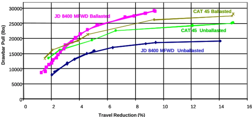
Another example of a pull-slip (travel reduction) plot is shown in figure 7 from Nebraska Tractor Test Laboratory (NTTL) data (for a complete vehicle). It also shows why dividing by the dynamic weight on the tractive device to create dimensionless ratios makes the comparisons more meaningful. A casual look at the travel reduction plots makes it appear that the John Deere 8400 ballasted tractor is outperforming the others, which in this case included both belt and rubber-tired tractors, both ballasted and unballasted.
JD 8400 MFWD Ballasted JD 8400 MFWD Unballasted CAT 45 Ballasted 0 5000 10000 15000 20000 25000 30000 0 2 4 6 8 10 12 14 16 Travel Reduction (%) Drawbar Pull (lbs) CAT 45 Unballasted JD 8400 MFWD Ballasted JD 8400 MFWD Unballasted CAT 45 Ballasted 0 5000 10000 15000 20000 25000 30000 0 2 4 6 8 10 12 14 16 CAT 45 Unballasted
Figure 7. Nebraska test drawbar pull comparison (ballasted and unballasted).
However, dividing the pull by the weight of the vehicles, in this case the total weight on the tractive devices produces a different picture (fig. 8).
0.00 0.20 0.40 0.60 0.80 1.00 1.20 0 2 4 6 8 10 12 14 16 Travel Reduction (%)
Vehicle Traction Ratio, VTR (pull / weight)
CAT 45 JD 8400 MFWD 0.00 0.20 0.40 0.60 0.80 1.00 1.20 0 2 4 6 8 10 12 14 16 CAT 45 JD 8400 MFWD
Figure 8. Nebraska test vehicle traction ratio comparison (ballasted and unballasted).
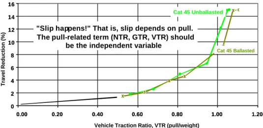
And there is still the question of which is the independent variable: travel reduction (slip), or pull (NTR or VTR)? This question cannot be answered here, as two definite groups support these two viewpoints, and each has supporting reasons. However, it is the authors' opinion that slip (travel reduction) happens because of a pull (NTR or VTR) being applied (fig. 9). This assumption will be used for the remainder of this paper.
0 2 4 6 8 10 12 14 16 0.00 0.20 0.40 0.60 0.80 1.00 1.20 Travel Reduction (%)
Vehicle Traction Ratio, VTR (pull/weight)
“Slip Happens!” That is, Slip depends upon pull.
“Slip Happens!” That is, Slip depends upon pull.
The pull related term, NTR, GTR, VTR should
The pull related term, NTR, GTR, VTR should
be the independent variable
be the independent variable
Cat 45 Unballasted Cat 45 Ballasted 0 2 4 6 8 10 12 14 16 0.00 0.20 0.40 0.60 0.80 1.00 1.20
"Slip happens!" That is, slip depends on pull. The pull-related term (NTR, GTR, VTR) should
be the independent variable
Cat 45 Unballasted
Cat 45 Ballasted
Figure 9. Nebraska test performance comparison with VTR as independent variable.
Tractive Efficiency
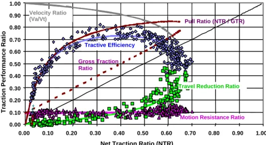
From a tractor drawbar power standpoint, tractive efficiency (TE) is the most important of the traction parameters. Figure 10 is a generalized plot of the traction relationships using the Brixius (1987) traction equations and net traction ratio (NTR) as the independent variable. For a properly ballasted and inflated agricultural tire, tractive efficiency (TE) tends to maximize at a net traction ratio (NTR) of approximately 0.40. This was also recognized by Dwyer (1984). Motion resistance ratio (MRR) tends to be a linear function of either slip or NTR unless slip sinkage becomes a factor.
0.00 0.10 0.20 0.30 0.40 0.50 0.60 0.70 0.80 0.90 1.00 0.00 0.10 0.20 0.30 0.40 0.50 0.60 0.70 0.80 0.90 1.00
Net Traction Ratio (NTR)
Traction Performance Ratio
Net Traction Ratio (NTR)
Travel Reduction Ratio)
Tractive Efficiency Ratio (TE)
(GTR - NTR) Motion Resistance Ratio
(1 - Va/Vt)
(GTR)
Gross Traction Ratio
Figure 10. Generalized traction relationship based on the Brixius (1987) traction equation.
There are travel and force losses that make up tractive "inefficiency" that do not have official
terminology. The simplest way to understand them is to look at them as a "velocity ratio" and a "pull ratio." In equation form: Ratio Velocity Ratio Pull Vt Va GTR NTR TE = × = (11)
The velocity ratio is shown as a function of net traction ratio (NTR) in figure 11. At zero NTR (zero pull) the actual velocity (Va) is about equal to the theoretical velocity (Vt), depending somewhat on the definition of "zero" slip (ASAE Standards, 2001b), and the velocity ratio is near unity. As net traction (pull)
increases, travel reduction (slip) increases, and the velocity ratio decreases. For a given traction device, velocity ratio losses depend on the characteristic shape of the pull-travel reduction curve.
Va/ Vt
Travel Reduction Ratio = (1 - Va /Vt)
0.00 0.10 0.20 0.30 0.40 0.50 0.60 0.70 0.80 0.90 1.00 0.00 0.10 0.20 0.30 0.40 0.50 0.60 0.70 0.80 0.90 1.00
Net Traction Ratio (NTR)
Traction Performance Rat
io Va= Actual Velocity Vt = Theoretical Velocity T E N T R G T R V a V t = Travel Reduction Ratio
0.00 0.10 0.20 0.30 0.40 0.50 0.60 0.70 0.80 0.90 1.00 0.00 0.10 0.20 0.30 0.40 0.50 0.60 0.70 0.80 0.90 1.00 Va = Actual velocity Vt = Theoretical velocity T E N T R G T R V a V t =
Velocity Ratio (Va/Vt)
(1 - Va/Vt)
Figure 11. Velocity losses in traction.
Pull ratio is shown as a function of NTR in figure 12. At zero net traction (pull), the ratio of net traction ratio (NTR) to gross traction ratio (GTR) approaches zero; the difference between GTR and NTR is the motion resistance ratio (MRR), which is in the range of 0.05 to 0.15. Due to motion resistance, the net traction ratio can never equal the gross traction ratio, and the pull ratio appro aches but never reaches unity.
Motion Resistance Ratio -NTR 0.00 0.10 0.20 0.30 0.40 0.50 0.60 0.70 0.80 0.90 1.00 0.00 0.10 0.20 0.30 0.40 0.50 0.60 0.70 0.80 0.90 1.00
Net Traction Ratio (NTR)
Traction Performance Ratio Motion Resistance Ratio
(GTR -NTR) Pull Ratio (NTR / GTR) 0.00 0.10 0.20 0.30 0.40 0.50 0.60 0.70 0.80 0.90 1.00 0.00 0.10 0.20 0.30 0.40 0.50 0.60 0.70 0.80 0.90 1.00 T E N T R G T R V a V t = T E N T R G T R V a V t =
Figure 12. Pull losses in traction.
Tractive efficiency is defined as output power / input power. It can also be expressed as the product of pull ratio and velocity ratio (eq. 11). Figure 13 shows how velocity ratio and pull ratio combine for overall tractive efficiency. The overall tractive efficiency cannot be greater than either the pull ratio or the velocity ratio, and thus it reaches a maximum value at NTR of between about 0.3 and 0.4 with radial-ply tires. It will be shown later that a similar range exists for belts.
Tractive Efficiency Ratio Velocity Ratio =Va/Vt
Travel Reduction Ratio = (1-Va/Vt)
Ratio = GTR -NTR Maximum Efficiency Point
Pull Ratio = NTR / GTR 0.00 0.10 0.20 0.30 0.40 0.50 0.60 0.70 0.80 0.90 1.00 0.00 0.10 0.20 0.30 0.40 0.50 0.60 0.70 0.80 0.90 1.00
Net Traction Ratio (NTR)
Traction Performance Ratio
T E N T R G T R V a V t = Tractive Efficiency Ratio Velocity Ratio (Va/Vt)
Travel Reduction Ratio
Motion Resistance Ratio (GTR - NTR) Maximum Efficiency Point
Pull Ratio (NTR / GTR) 0.00 0.10 0.20 0.30 0.40 0.50 0.60 0.70 0.80 0.90 1.00 0.00 0.10 0.20 0.30 0.40 0.50 0.60 0.70 0.80 0.90 1.00 T E N T R G T R V a V t = (1 - Va/Vt)
Figure 13. Overall tractive efficiency with velocity and pull losses.
Pull ratio, velocity ratio, and tractive efficiency are shown for real data in figure 14. Data is for radial-ply tires in medium (tilled) tractive conditions. The curves are the result of regression analysis of the field test data. Both velocity (travel reduction) and pull (motion resistance) losses contribute to the overall tractive efficiency. 0.00 0.10 0.20 0.30 0.40 0.50 0.60 0.70 0.80 0.90 1.00 0.00 0.10 0.20 0.30 0.40 0.50 0.60 0.70 0.80 0.90 1.00
Net Traction Ratio (NTR)
Traction Performance Ratio
Gross Traction Ratio
Travel Reduction Ratio Pull Ratio (NTR / GTR)
Motion Resistance Ratio Velocity Ratio
(Va/Vt)
Tractive Efficiency
Figure 14. Traction data with regression and loss curves. Tire = Goodyear 20.8R42 DT/DT710 dual. Surface = Lon's tilled (seeded).
The same power loss data can be viewed in a travel reduction (slip) based plot (fig. 15), but it is not so easy or intuitive to relate the losses to travel reduction. This is probably because we are looking at losses as a function of one of the losses itself. This again supports NTR as being the independent variable.
Tractive Efficiency Net Traction Ratio Gross Traction Ratio
Pull Ratio = NTR/GTR 0.00 0.10 0.20 0.30 0.40 0.50 0.60 0.70 0.80 0.90 1.00 0 10 20 30 40 50 Travel Reduction (%)
Traction Performance Ratio
Velocity Ratio =Va/Vt T E N T R G T R V a V t =
Motion Resistance Ratio = GTR -NTR
Tractive Efficiency Net Traction Ratio
Gross Traction Ratio
Pull Ratio (NTR/GTR) 0.00 0.10 0.20 0.30 0.40 0.50 0.60 0.70 0.80 0.90 1.00 0 10 20 30 40 50
Velocity Ratio (Va/Vt)
T E N T R G T R V a V t =
Motion Resistance Ratio (GTR - NTR)
Figure 15. Traction losses with travel reduction (slip) as independent variable.
Regression Analysis
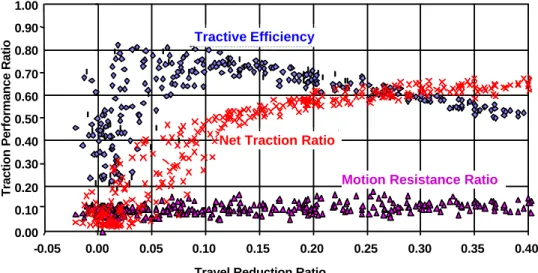
Typical traction data plots are shown in figures 16 and 17. Figure 16 shows an example of the traditional plot with travel reduction as the independent variable. Each point on the plot represents the average of 1.5 seconds of data sampled at approximately 50 Hz. Considerable data scatter occurs,
especially at the lower values of travel reduction. Most of the data scatter can probably be attributed to the difficulty in measuring actual travel speed (Va). This is normally done with a fifth wheel or a radar device. Variations in Va affect the travel reduction calculation, especially at values near zero. Thus, the apparent vertical scatter of the NTR (pull) data is actually a horizontal scatter of the travel reduction data.
Variations in the measurement of actual travel speed (Va) also affect the calculated tractive efficiency, which shows a similar scatter at the lower travel reduction values. Note that while the motion resistance ratio (MRR) is also a calculated value, it does not show the same increase in scatter at the low travel reduction values. This is because motion resistance is calculated from gross traction and net traction, which do not show a variation with travel reduction. In addition, as motion resistance ratio (MRR) is nearly constant with travel reduction, any variations caused by variations in the slip calculation will be hidden as the points simply move sideways.
The resulting scatter of the d ata makes it difficult to determine significant values to use to compare performance of two (or more) tractive devices. This is one reason that regression analysis of the data is commonly used. The method used by the authors was developed with the assistance of Dr. Shrini Upadhyaya of the University of California, Davis (Upadhyaya et al., 1988). His Quick Basic program for Macintosh was converted to run in Excel Visual Basic. The original method included a regression of GTR and NTR as a function of slip (travel reduction). It was modified in the conversion to Excel Visual Basic to regress NTR and MRR. The method determines a regression curve for NTR and MRR as a function of travel reduction (slip):
NTR = DA × [1 - exp(-C0 × TRR × 100)] (12)
MRR = TA + AB × TRR (13)
Following determination of the regression coefficients, GTR and TE can be calculated as: GTR = NTR + MRR
TE = NTR × (1 - TRR) / GTR
In the following examples (figs. 16 through 19), each data point represents the average for 1.5 seconds. This example shows the merging of three replications of the test run. Also shown as a smooth curve are the
results of a regression of the NTR and MRR data. These are examples only, and all subsequent comparisons are made using the regression coefficients.
0.00 0.10 0.20 0.30 0.40 0.50 0.60 0.70 0.80 0.90 1.00 -0.05 0.00 0.05 0.10 0.15 0.20 0.25 0.30 0.35 0.40 Travel Reduction Ratio
Traction Performance Ratio
Tractive Efficiency
Net Traction Ratio
Motion Resistance Ratio
Figure 16. Traditional slip plot with experimental data. Tire = 20.8R42 dual. Surface = Lon's tilled (seeded).
1.00
-0.05 0.00 0.05 0.10 0.15 0.20 0.25 0.30 0.35 0.40 Travel Reduction Ratio
0.00 0.10 0.20 0.30 0.40 0.50 0.60 0.70 0.80 0.90
Traction Performance Ratio
NTR = 0.664(1-exp-0.098(TRR)) MRR = 0.090 + 0.001(TRR))
Motion Resistance Ratio
Tractive Efficiency
Net Traction Ratio
Figure 17. Traditional slip plot of traction data with regression curves. Tire = 20.8R42 dual. Surface = Lon's tilled (seeded).
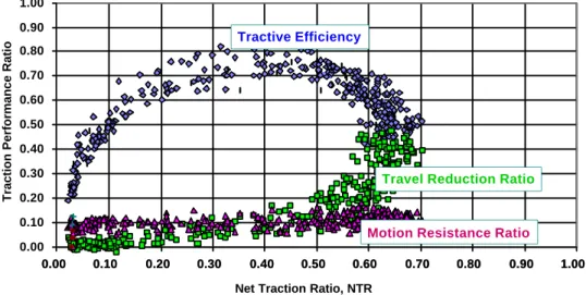
0.00 0.10 0.20 0.30 0.40 0.50 0.60 0.70 0.80 0.90 1.00 0.00 0.10 0.20 0.30 0.40 0.50 0.60 0.70 0.80 0.90 1.00 0.00 0.10 0.20 0.30 0.40 0.50 0.60 0.70 0.80 0.90 1.00
Net Traction Ratio, NTR
Traction Performance Ratio
Tractive Efficiency
Motion Resistance Ratio
Travel Reduction Ratio
Figure 18. Experimental data with net traction ratio as independent variable. Tire = Goodyear 20.8R42 DT/DT710 dual. Surface = Lon's tilled (seeded).
0.00 0.10 0.20 0.30 0.40 0.50 0.60 0.70 0.80 0.90 1.00 Net Traction Ratio, NTR
0.00 0.10 0.20 0.30 0.40 0.50 0.60 0.70 0.80 0.90 1.00
Traction Performance Ratio
NTR = 0.664(1-exp-0.098(TRR)) MR = 0.090 + 0.001(TRR))
Tractive Efficiency
Motion Resistance Ratio
Travel Reduction Ratio
Figure 19. Experimental data and regression curves with net traction ratio as independent variable. Tire = Goodyear 20.8R42 DT/DT710 dual. Surface = Lon's tilled (seeded).
4. Traction Testing
Traction testing involves operating a traction device (wheel or belt) in the soil and making measurements of its performance. Four dynamic (on the go) measurements are required:
• Input torque (T) • Input speed (ω) • Output force (NT) • Output speed (Va)
Additionally, the dynamic weight (ground reaction force) must be known, measured, or calculated. This will usually depend on the design of the traction test device. If a single-wheel tester is used, it can be designed such that the dynamic weight reaction force is equal to that measured statically.
Single-Wheel Testing
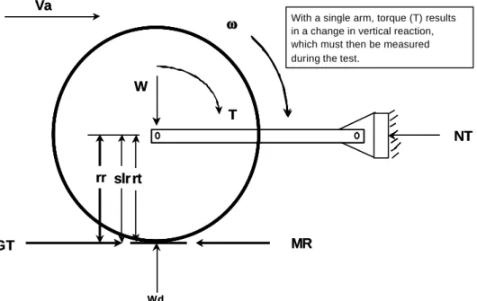
The simplest device for a traction test of a wheeled device requires support ing the moving wheel, applying the required torque, and measuring the developed force (net traction). However, there are various ways this can be accomplished, with varying levels of complexity. Some devices can operate only in soil bins, i.e., bring the soil to the device, while others are operated in the field. In some cases, testing is done using complete vehicles, with the tractive device being the drive wheels or tracks. The most basic traction testing device is shown in figure 20.
GT MR slr rr NT T W Va ω ω Wd rt GT MR slr rr NT T W Va ω ω Wd
With a single arm, torque (T) results in a change in vertical reaction, which must then be measured during the test.
rt
Figure 20. Simplest form of single-wheel tester.
With the single-link device (fig. 20), a change in input torque (T) results in a change in vertical force reaction (Wd), which then must be measured dynamically during the test (normally set and measured statically). Figure 21 shows a modification using two parallel links; this eliminates the weight transfer effect but may result in more difficult measurement of NT and T. Actually, there are two alternatives for measuring torque: directly measuring the input torque, or determining torque from the measurement of NT. Net traction is the vector sum of the two reaction forces; the input torque can be determined by the difference in the two reaction forces multiplied by the distance between the links.
GT MR slr rr T W Va ω ω Wd NT/2
With parallel arms, there is no change in vertical reaction as torque is applied.
NT/2
Net traction can be calculated as the sum of the reaction forces. Torque can be calculated as the difference in the forces multiplied by the distance between the arms.
rt GT MR slr rr T W Va ω ω Wd NT/2 NT/2 rt
Figure 21. Single-wheel tester with parallel arms.
Most single -wheel testers use the mechanism shown in figure 22. Torque is measured at the input to the wheel. GT MR slr rr T W Va ω ω Wd
With parallel arms, there is no change in vertical reaction as torque is applied (i.e., W = Wd)
NT rt GT MR slr rr T W Va ω ω Wd NT rt
Figure 22. Parallel arm single-wheel tester with direct measurement of NT.
Using Tractors to Test Tires
While single-wheel testing is conceptually the most simple and direct approach to testing a traction device, a tractor can be used to test tires (fig. 23) and in fact is the most common method to test belts. Use of a tractor means that two of the traction devices are actually under test. When a tractor is used, some method must be used to determine the dynamic weight on the drive wheels (due to weight transfer when pulling), and in the case of full four-wheel drive, some method must be used to determine the net traction
(pull) developed by each axle. For a tractor with mechanical front-wheel drive, it is nearly impossible to conduct a pure traction test because the dynamic weights and the net traction developed by the front axle need to be determined, and the front and rear axles are typically equipped with different size tires.
c MR slr rr T RWS ω ω GT Va FWS MRf RWD Wb P Dh FWD rt c MR slr rr T RWS ω ω GT Va MRf RWD Wb P Dh FWD rt
Figure 23. Two-wheel drive tractor used as tire tester. Front static weight (FWS) is usually set to be approximately 20% of total tractor weight.
When using a tractor to test tires, it is best to use a two -wheel drive model while measuring or
calculating the front axle dynamic weight and motion resistance force. Since there is no torque input at the front axle, i.e., no gross traction force, the motion resistance force is equal to a negative net traction and is subtracted from the measured drawbar pull for traction calculations. (Note: For force/moment calculations, the total drawbar pull should be used.)
When using a complete tractor to test tires or belts, certain measurements are needed or calculated before testing can begin. Front (FWS) and rear (RWS) static weights must be adjusted and measured. It is helpful if the static front weight (FWS) is kept relatively low (similar to that required for implements
attached to the drawbar) and at a constant percent of the total tractor weight. Use of front and rear suitcase-style weights (fig. 23) facilitates obtaining the correct weight on the test tires (rear) and the desired weight distribution. Drawbar height (Dh) and wheelbase (Wb) are measured for use in calculating weight transfer to the rear and rear dynamic weight (RWD). The rolling radius (rr) of the tire under test is determined by a "free roll", that is, zero drawbar pull and zero net traction, as described by method 2 (in section 2 of this paper under "Travel Reduction Ratio"). If the free roll is determined on a hard surface, then the front motion resistance (MRf) is ignored.
During a test, the input axle torque (T) and speed of the axle (ω) are measured along with the drawbar pull (P) and actual travel speed (Va). The rear dynamic weight (RWD) is calculated from the rear static weight (RWS) and the weight transfer from the front. In the calculations, an attempt is made to calculate (estimate) the front motion resistance force (MRf), which is the difference between drawbar pull (P) and the net traction (NT) output from the tires under test. In addition, recognize that there are actually at least two tires under test.
The rear dynamic weight (RWD) of the tractor is calculated as the sum of the static rear weight (RWS) and the weight transfer. Weight transfer is calculated as P × Dh/Wb. Since the drawbar pull is horizontal, any weight transferred to the rear axle is subtracted from the front, and the front dynamic weight (FWD) is calculated by subtracting the weight transfer from the front static weight (FWS). This is then used to estimate the front motion resistance. The method used to calculate front motion resistance (MRf) is a circular reference in a spreadsheet. Assume that the front motion resistance ratio is equal to that calculated at the rear. This calculation can also be done on-the-go in a data acquisition program. The steps taken are: 1. Initially assume that the dynamic front weight (FWD) is equal to the static front weight (FWS).
2. Assume a front motion resistance ratio (MRR) as a starting point.
3. Calculate front motion resistance force (MRf) and add it to the net traction force (initially equal to drawbar pull).
4. Recalculate the new rear MRR (from within the traction calculations using new NTR). 5. Use the newly calculated rear MRR to calculate the new front (MRf).
6. Loop back until the data do not change (to whatever significance you are operating, usually the third decimal place). At this point, the front MRR is equal to the rear MRR, and the net traction force has been adjusted for what it is estimated to be required to push the front wheels through the field. Note that this means that net traction will be higher than the measured drawbar pull (considering the number of tires under test).
Traction testing in the field always requires a way to apply a load to the tire test tractor. It is possible to take traditional drawbar loading units that might be used on a hard surface to the field and use them. However, there are problems in doing this. Relatively heavy load units are required for the high draft loads, which limits the minimum drawbar pull to the motion resistance of the load unit, and as a result, lower portions of the pull-travel reduction curve cannot be attained. It is preferred to use a second live tractor in combination with an implement (fig. 24). An implement that operates narrow and deep is preferred, to limit the area of the test field that is disturbed. The travel speed of the load tractor (gear and engine speed, set at about 3/4 throttle to allow adjustment up and down) is set to match that of the test tractor. The implement is operated at a depth that the load tractor can pull, and the drawbar pull applied to the test tractor is adjusted using the throttle of the load tractor. Throttling back the load tractor increases the load on the test tractor, as the test tractor is thereby caused to pull more of the implement load. Increasing the throttle setting on the load tractor causes it to overtake the test tractor, reducing the drawbar pull as the load tractor pulls the implement. The disadvantage of this method is that it requires two operators and a method to communicate between the two as the load is adjusted.
c
RWS Va
FWS
RWD FWD
Tire Test Tractor
Vt Dh c Load Tractor Dh c c Wb
Figure 24. Tire test tractor with powered tractor and implement as load unit.
Speed Effects
The speed or gear of the test tractor is set to one that can develop full torque (desired wheel slip) to the test tires. Other methods can be used, depending on the flexibility of the transmission of the tire test tractor, but it is necessary to go from the minimum torque necessary to self-propel the tractor to that which
develops in the range of 30% to 40% travel reduction. Depending on the power of the tire test tractor and its weight (the weight on the traction device being tested), this torque could be developed over a range of travel speeds. This leads to the question of speed effects in traction testing.
Figure 25 shows the results of a traction test conducted over an extreme (for agricultural tractors) range of travel speeds. The test was conducted under self-propelled conditions, i.e., net traction is zero (except for possible front axle effects). The test showed a slight increase in MRR with speed, but little change over the normal range of tractor field speeds. It is easy to be misled by the extra power required to drive the tractor at the higher speeds, as the axle power ranged from about 5 to 35 kW while the MRR was virtually constant.
Theoretical (no slip) Travel Speed (Vt, m/s)
Motion Resistance Ratio
0.00 0.10 0.20 0.30 0.40 0.50 0.60 0.70 0.80 0.90 1.00 0.0 1.0 2.0 3.0 4.0 5.0 6.0 0.0 5.0 10.0 15.0 20.0 25.0 30.0 35.0 40.0 Axle Power (kW) 0.00 0.10 0.20 0.30 0.40 0.50 0.60 0.70 0.80 0.90 1.00 0.0 1.0 2.0 3.0 4.0 5.0 6.0 0.0 5.0 10.0 15.0 20.0 25.0 30.0 35.0 40.0 Axle Power, (kW) 4.5 m/s = 10 mph MRR = 0.0079(Vt) + 0.0806
Figure 25. Speed effects on motion resistance. Tire = 710/70R38 on loose soil.
5. Traction Performance
The following series of figures shows typical traction test curves for different soils, tire size and
pressure, load on the tires, and belts vs. tires. All curves were developed using the regression methodology on data from actual traction tests. Figure 26 is an example that shows how to interpret the traction plots. As indicated in figure 26, each tractive efficiency curve has a peak value, a value of net traction ratio where the peak occurs, and an arbitrary efficient pull (net traction) range. Also shown is the resulting travel reduction, including maximum pull (net traction ratio), which is usually limited by the test engineer. Tractive
efficiency tends to peak near an NTR of 0.4 for tires and 0.5 for belts.
Traction Performance Ratios
0.0 0.1 0.2 0.3 0.4 0.5 0.6 0.7 0.8 0.9 1.0 0.00 0.10 0.20 0.30 0.40 0.50 0.60 0.70 0.80 0.90 1.00 Net Traction Ratio (NTR)
Efficient Pull Range
0.0 0.1 0.2 0.3 0.4 0.5 0.6 0.7 0.8 0.9 1.0 0.00 0.10 0.20 0.30 0.40 0.50 0.60 0.70 0.80 0.90 1.00 Travel Reduction Ratio
Tractive Efficiency Ratio Peak TE
Pull @ Max T E
Max Pull (slip limited)
Figure 26. How to interpret traction plots (performance of 20.8R42 dual tires on three surfaces).
Effects of Soil
Figure 27 shows the performance of 20.8R42 dual tires on three tractive surfaces. Note that the peak tractive efficiency is reduced as the soil becomes softer and looser, but that the peak occurs at a net traction ratio of approximately 0.4 on all soils. Maximum NTR is also reduced as the soil becomes less firm (lower net traction at the same travel reduction).
Traction Performance Ratios
1.00
Net Traction Ratio (NTR) 0.00 0.10 0.20 0.30 0.40 0.50 0.60 0.70 0.80 0.90 0.00 0.10 0.20 0.30 0.40 0.50 0.60 0.70 0.80 0.90 1.00
Travel Reduction Ratio
Untilled
Tilled Subsoiled
Tractive Efficiency
Figure 27. Performance of 20.8R42 dual tires on three surfaces (8300 kg axle load, 83 kPa tire pressure).
Effects of Tire Pressure
Figure 28 is an example of operating tires that were over-inflated for their load capacities compared to correctly inflated tires. Maximum tractive efficiency is reduced as well as the maximum net traction ratio. While the maximum tractive efficiency is only reduced about 5 percentage points, the effect on vehicle performance may be significantly greater depending on how implements are matched to the tractor. For example, at an NTR of 0.5, more than 10 percentage points of difference will result in about 17% difference in drawbar power and significantly higher travel reduction.
1.00
Traction Performance Ratios
0.00 0.10 0.20 0.30 0.40 0.50 0.60 0.70 0.80 0.90 0.00 0.10 0.20 0.30 0.40 0.50 0.60 0.70 0.80 0.90 1.00
Net Traction Ration (NTR) Tractive Efficiency
Travel Reduction Ratio
6 psi load @ 6 psi (correct) (41 kPa) (41 kPa)
6 psi load @ 28 psi (41 kPa) (193 kPa)
Figure 28. Performance of single tire (Firestone 710/70R38 ATR) at two inflation pressures in tilled (loose) tractive conditions.
Effects of Tire Size
Performance of two tire sizes at the correct inflation pressure is shown in figure 29. The larger diameter 520/85R46 tire shows significantly higher power efficiency at the same slip. This demonstrates that wider tires (710/70R38) have greater motion resistance loss (both operating at about the same travel reduction). Both provide similar maximum pull capability, which may give the operator the impression that there is no performance difference between the tires.
1.00
1.00 Net Traction Ration (NTR)
0.00 0.10 0.20 0.30 0.40 0.50 0.60 0.70 0.80 0.90 0.00 0.10 0.20 0.30 0.40 0.50 0.60 0.70 0.80 0.90
Traction Performance Ratios
Tractive Efficiency
Travel Reduction Ratio 710/70R38, 6 psi load @ 6 psi (correct)
(41kPa) (41kPa)
520/85R46, 8 psi load @ 8 psi (correct) (55kPa) (55kPa)
Figure 29. Performance of two sizes of single tires at correct inflation pressures in tilled (loose) tractive conditions.
Effects of Load on Tire
Figure 30 shows performance of the same size tire with correct inflation pressure for different weights. Using the correct inflation pressure for the weight allows the tire to operate at its design deflection ratio where optimum performance is obtained (Zoz and Turner, 1994). Maximum tractive efficiency is achieved at about the same net traction ratio for each weight. It should be noted that this means pull in proportion to the dynamic weight. In other words, if only the weight is changed, then performance may suffer from not operating at the optimum NTR.
1.00
Net Traction Ratio (NTR) 0.00 0.10 0.20 0.30 0.40 0.50 0.60 0.70 0.80 0.90 0.00 0.10 0.20 0.30 0.40 0.50 0.60 0.70 0.80 0.90 1.00
Traction Performance Ratios
Tractive Efficiency
16 psi load @ 16 psi (correct) (110kPa) (110kPa)
8 psi load @ 8 psi (correct) (55kPa) (55kPa)
Travel Reduction Ratio
Figure 30. Performance of single tire (Goodyear 520/85R46 DTR) at two weights with correct pressures in tilled (loose) tractive conditions.
Belt and Tire Comparisons
To determine the effect of belt width on tractive performance, three belts of 400, 630, and 810 mm width (16, 25, and 32 in.) were tested from one manufacturer. A 400 mm (16 in.) belt was tested from a second manufacturer. During these tests, a set of 20.8R42 dual tires was also compared. Tests were conducted on untilled and tilled tractive conditions. In the process of testing, a subsoiler was used on the load tractor to provide a portion of the load. This tilled pass provided a soft subsoiled condition on which further tractive comparisons were made.
Figures 31 through 33 show the performance of the three belt widths in comparison to the dual tires on three surfaces. Under firm untilled conditions (fig. 31), there is little performance difference between the four treatments at normal field pulls (NTR approximately 0.4 to 0.5). Dual tires dropped off at the higher pulls, and the wider belt provides higher maximum NTR (limited by travel reduction).
1.00
Net Traction Ratio (NTR)
Traction Performance Ratios
0.00 0.10 0.20 0.30 0.40 0.50 0.60 0.70 0.80 0.90 0.00 0.10 0.20 0.30 0.40 0.50 0.60 0.70 0.80 0.90 1.00 1.00 0.00 0.10 0.20 0.30 0.40 0.50 0.60 0.70 0.80 0.90 0.00 0.10 0.20 0.30 0.40 0.50 0.60 0.70 0.80 0.90 1.00 Travel Reduction Ratio
Cat 25”(630mm) 20.8R42 Dual Tires
Tractive Efficiency
Cat 32”(810mm)
Cat 16”(400mm)
Figure 31. Belt width comparison on firm untilled soil (belted tractor total weight = 12700 kg; wheel tractor axle weight = 8303 kg).
As the tractive conditions become softer and looser, the differences are mo re evident between belts and tires, while the belts maintain their relative position with each other (figs. 32 and 33). Note that the
maximum tractive efficiency for tires still comes at NTR of about 0.4, while the belts tend to maximize at a slightly higher pull (approximately 0.5 NTR) and demonstrate a wider range of pulls at near-maximum tractive efficiency. It should be noted that these tests were all carried out with a minimum of steering. Matching implements at higher VTR on the skid steer belted machine may hinder steering control under load. 1.00 0.00 0.10 0.20 0.30 0.40 0.50 0.60 0.70 0.80 0.90 0.00 0.10 0.20 0.30 0.40 0.50 0.60 0.70 0.80 0.90 1.00
Net Traction Ratio (NTR)
Traction Performance Ratios
20.8R42 Duals
Cat 16”(400mm)
Travel Reduction Ratio
Cat 32”(810mm)
Tractive Efficiency
Cat 25”(630mm)
Figure 32. Belt width comparison on tilled soil (belted tractor total weight = 12700 kg; wheel tractor axle weight = 8303 kg).
1.00
Traction Performance Ratios
0.00 0.10 0.20 0.30 0.40 0.50 0.60 0.70 0.80 0.90 0.00 0.10 0.20 0.30 0.40 0.50 0.60 0.70 0.80 0.90 1.00 Net Traction Ratio (NTR)
Tractive Efficiency
Cat 32”(810mm)
Cat 25”(630mm) Cat 16”(400mm)
20.8R42 Duals
Travel Reduction Ratio
Figure 33. Belt width compari son on subsoiled land (belted tractor total weight = 12700 kg; wheel tractor axle weight = 8303 kg).
Two manufacturers' 400 mm (16 in.) belts are compared in figures 34 through 36. Little difference was observed in performance between the two belts on the three surfaces tested. It should also be noted that under the firm untilled conditions, the correctly inflated 20.8R42 dual tires equaled or outperformed the 400 mm (16 in.) belts. 1.00 0.00 0.10 0.20 0.30 0.40 0.50 0.60 0.70 0.80 0.90 0.00 0.10 0.20 0.30 0.40 0.50 0.60 0.70 0.80 0.90 1.00
Net Traction Ratio (NTR)
Traction Performance Ratios
Tractive Efficiency
Cat 16”(400mm)
20.8R42 Duals
Travel Reduction Ratio GY 16”(400mm)
Figure 34. Belt manufacturer comparison on firm untilled soil (belted tractor total weight = 12700 kg; wheel tractor axle weight = 8303 kg).
1.00
Traction Performance Ratios
0.00 0.10 0.20 0.30 0.40 0.50 0.60 0.70 0.80 0.90 0.00 0.10 0.20 0.30 0.40 0.50 0.60 0.70 0.80 0.90 1.00
Net Traction Ration (NTR)
Travel Reduction Ratio Tractive Efficiency
20.8R42 Duals
GY 16”(400mm) Cat 16”(400mm)
Figure 35. Belt manufacturer comparison on tilled soil (belted tractor total weight = 12700 kg; wheel tractor axle weight = 8303 kg).
1.00
1.00 Net Traction Ratio (NTR)
0.00 0.10 0.20 0.30 0.40 0.50 0.60 0.70 0.80 0.90 0.00 0.10 0.20 0.30 0.40 0.50 0.60 0.70 0.80 0.90
Traction Performance Ratios
20.8R42 Duals
Tractive Efficiency
Cat 16”(400mm)
Travel Reduction Ratio G Y 16”(400mm)
Figure 36. Belt manufacturer comparison in subsoiled tractive condition (belted tractor total weight = 12700 kg; wheel tractor axle weight = 8303 kg).
Figures 37 and 38, respectively, compare the performance of 630 mm (25 in.) belts and 20.8R42 dual tires on the three surfaces tested. As the soil becomes softer, dual tires demonstrate greater difference in tractive efficiency than does the belt.