RESEARCH SEMINAR IN INTERNATIONAL ECONOMICS
Gerald R. Ford School of Public PolicyThe University of Michigan Ann Arbor, Michigan 48109-3091
Discussion Paper No. 596
Decentralized Borrowing and Centralized
Default
Yun Jung Kim
University of MichiganJing Zhang
University of MichiganApril 9, 2010
Recent RSIE Discussion Papers are available on the World Wide Web at: http://www.fordschool.umich.edu/rsie/workingpapers/wp.html
Decentralized Borrowing and Centralized
Default
Yun Jung Kim
∗Jing Zhang
†University of Michigan University of Michigan
April 9, 2010
Abstract
In the past, foreign borrowing by developing countries was comprised almost en-tirely of government borrowing. Recently, private firms and individuals in developing countries borrow substantially from foreign lenders. It is not clear whether the observed increase in private sector borrowing leads to overborrowing and frequent defaults by governments in developing countries. In this paper, we develop a tractable quantitative model in which private agents decide how much to borrow but the government decides whether to default. The model with decentralized borrowing increases aggregate credit costs and sovereign default risk, and reduces aggregate welfare, relative to a model with centralized borrowing. Private agents do not internalize the effect of their borrowing on economy-wide credit costs and thus would like to borrow more than the socially efficient level. Depending on the severity of default penalties, decentralized borrowing may lead to either too much or too little debt in equilibrium. The introduction of decentralized borrowing substantially improves the model’s empirical fit in terms of matching observed debt levels and default rates.
JEL Classification Number: F32, F34, F41
Keywords: Sovereign Default, Sovereign Debt, Private Borrowing, Capital Flows
∗Department of Economics, University of Michigan, 611 Tappan St., Ann Arbor, MI, 48109. Email:
†Department of Economics, University of Michigan, 611 Tappan St., Ann Arbor, MI, 48109. Email:
1
Introduction
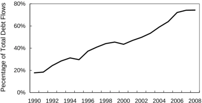
In the past, foreign borrowing by developing countries was comprised almost entirely of government borrowing. Recently, owing in part to efforts by international institutions to promote economic growth, private firms and individuals in developing countries borrow sub-stantially from foreign lenders. As shown in Figure 1, private borrowing rose from only 18 percent of total borrowing from foreign lenders in 1990 to more than 70 percent in 2008.1 Foreign lenders often price private loans with macroeconomic indicators of developing coun-tries instead of characteristics of private borrowers, because governments can block private debt repayments or nationalize private debts if such an action is perceived as welfare im-proving.2 The surge in private borrowing and the lending practices of foreign lenders have
been blamed for causing overborrowing and frequent defaults by developing countries. Figure 1: Debt Flows to Private Sectors of Developing Countries
0% 20% 40% 60% 80% 1990 1992 1994 1996 1998 2000 2002 2004 2006 2008
Pecentage of Total Debt Flows
This paper investigates the effect of decentralized borrowing in a tractable quantita-tive model in which private agents decide how much to borrow but the government decides whether to default. We have three main findings. First, the model with decentralized bor-rowing increases aggregate credit costs and sovereign default risk, and reduces aggregate welfare, relative to the model with centralized borrowing where the government also decides how much to borrow. Second, depending on the severity of default penalties, decentralized borrowing may lead to either too much or too little debt in equilibrium. Third, the intro-duction of decentralized borrowing substantially improves the model’s empirical fit in terms of matching observed debt levels and default rates.
1Data come fromGlobal Development Finance.
2Chile’s debt nationalization in 1982 is an example. For more detailed discussion, see Fernandez-Arias
Our model extends the classic centralized-borrowing framework of Eaton and Gersovitz (1981) by decentralizing borrowing decisions. A continuum of identical households borrow from foreign lenders in terms of non-contingent debt to smooth their aggregate income shocks. A benevolent government decides on whether to enforce debt repayments to maximize the welfare of the representative household. If the government defaults, the country loses access to international financial markets and suffers from income losses for some stochastic periods. Foreign lenders offer the households a bond price schedule which depends on the level of aggregate borrowing instead of individual borrowing, because aggregate borrowing, together with the aggregate income shock, determines the default probability. Our centralized default setup captures the lending practices to developing countries based on aggregate indicators.3 We first contrast the model mechanisms determining the equilibrium level of debt under decentralized borrowing with those under centralized borrowing. Under centralized borrow-ing, the government takes into account the adverse effect of an extra unit of debt on credit costs and on next-period default probabilities when choosing debt contracts. In contrast, individual households fail to internalize the adverse effect of their borrowing on aggregate credit costs and next-period default probabilities, and would like to overborrow. The over-borrowing incentive lowers the repayment welfare and thus increases the default likelihood of the government. Consequently, the bond price schedule is lower under decentralized bor-rowing, which tends to reduce the debt level. The relative strength of the overborrowing incentive and the bond price schedule effect determines the equilibrium level of debt.
To examine quantitative implications of decentralized borrowing, we then parameterize the model, in particular, the default penalties. Following Arellano (2008), we assume that income losses after default are disproportionately large under good income shocks, allowing the default model to generate the empirically reasonable default rate. Under the benchmark parameter values, we find that decentralized borrowing substantially increases credit costs, the default rate and the equilibrium level of debt, and reduces the country’s welfare relative to centralized borrowing. All these implications except the one on the equilibrium level of debt are robust to alternative parameter values of default penalties.
Decentralized borrowing increases the equilibrium level of debt under lenient default penalties, but lowers it under severe default penalties, relative to centralized borrowing.4 Consider the two effects determining the equilibrium level of debt. The overborrowing incen-3In our model, decentralized borrowing and decentralized default generate the same outcomes as
central-ized borrowing and centralcentral-ized default.
4If income losses after default are a constant fraction of the income shock, the decentralized borrowing
tive arises from the failure of individual households to internalize the effect of their borrowing on the bond price. Thus, the overborrowing incentive is strong when the bond price declines rapidly with debt, i.e., when default penalties are lenient. The bond price schedule effect arises from the failure of individual households to internalize the effect of their borrowing on the government’s default choices. Thus, the bond price schedule effect is strong when the government wants to avoid default badly, i.e., when default penalties are severe. Therefore, when default penalties are lenient, the overborrowing effect dominates, implying equilibrium overborrowing. When default penalties are severe, the bond price schedule effect dominates, implying equilibrium underborrowing.
Decentralized borrowing improves the model’s empirical fit in many dimensions. In par-ticular, decentralized borrowing has an inherent mechanism to simultaneously increase both the debt level and the default rate in equilibrium. Individual households tend to borrow reck-lessly due to the failure to internalize the adverse effect of their borrowing, and consequently the government finds default attractive more often. In contrast, the model with centralized borrowing can improve one dimension of the model fit at the expense of the other. When both models are calibrated to match the observed default rate, the centralized borrowing model generates an extremely low debt to income ratio of 5%, but this ratio is 17% under the decentralized borrowing model.
Our work is closely related to Uribe (2006), who shows that regardless of whether a debt limit is imposed at the country level or at the individual level, the equilibrium level of debt is the same. In his analysis, the debt limit and the interest rate are exogenously specified, and there is no default risk. By contrast, in our model, the presence of default risk endoge-nizes both the interest rate and the debt limit. In particular, the overborrowing incentive of individual agents drives up sovereign default risk and the interest rate. Consequently, decen-tralized borrowing generates an equilibrium level of debt different from cendecen-tralized borrowing in general.
Our work is related to the recent theoretical literature on private international borrow-ing. Jeske (2006) and Wright (2006) study the effect of private borrowing under complete markets, where no default occurs in equilibrium. In contrast, we consider an incomplete markets environment5 and allow equilibrium default. Broner and Ventura (2010) analyze an environment with both domestic and international trade of contingent claims among private agents. They assume that the government, when deciding whether to enforce the claims, 5Bai and Zhang (2010) show that both incomplete markets and default risk are important to account for
cannot discriminate between domestic and foreign creditors. We implicitly allow discrimi-nation; the government always enforces repayments among domestic agents but can choose not to enforce repayments to foreigners.
Our model builds on the classic sovereign default framework of Eaton and Gersovitz (1981) and recent quantitative research on sovereign debt. Arellano (2008), Aguiar and Gopinath (2006), Bai and Zhang (2009), Cuadra and Sapriza (2008) and Yue (2009) assume that the government makes both borrowing and default decisions. Mendoza and Yue (2008), on the other hand, allow private firms to borrow abroad to finance their working capital and a government to borrow on behalf of households, while the default decision is made by the government. Their focus is different from ours: they aim to generate endogenous output costs of default.
The remainder of the paper is organized as follows. Section 2 presents the model with decentralized borrowing. In section 3, we compare the quantitative implications of the models with decentralized and centralized borrowing. Section 4 investigates how different default penalties affect the quantitative results, in particular, the equilibrium debt level. We conclude in section 5.
2
Models
This section presents a dynamic stochastic general equilibrium model of decentralized bor-rowing and centralized default in which borbor-rowing decisions are made by individual house-holds and default decisions are made by a government. This setup is intended to capture an environment in which borrowing decisions are made by private agents and lending decisions of foreign lenders are guided by aggregate indicators rather than individual borrowers’ ability to repay.
2.1
Model with Decentralized Borrowing
The model economy consists of three types of agents: a continuum of identical households and a sovereign government in a small open economy, and foreign lenders. The households re-ceive stochastic aggregate income shocksy, which follow a Markov process with the transition function f(y0, y). In order to smooth income shocks, the households trade non-contingent bonds b with risk-neutral foreign lenders. The benevolent government, maximizing its rep-resentative household’s welfare, decides whether to enforce foreign debt contracts. In each
period, the country is either in the normal phase with access to international financial mar-kets or in the penalty phase without access to financial marmar-kets.
The timing is as follows. At the beginning of each period, the income shockyis realized. If the country is in the normal phase, the government decides whether to enforce the repayment of outstanding foreign debt B.6 If the government enforces debt contracts, the households
repay their debt b and decide on consumption c and next-period debt b0. If the government defaults, the households do not to repay their debt, and the economy goes into the penalty phase. The country in the penalty phase suffers from income loss and has probability θ of reverting to the normal phase each period.
Government
At the beginning of the normal period, the benevolent government observes current income shock y and aggregate foreign debt B. The government decides whether to enforce debt contracts to maximize the representative household’s welfare. This welfare is given byvD(y) if the government chooses to default, and vR(B, y,Γ (B, y)) if the government chooses to enforce the repayment with an anticipation that the economy will borrowB0 = Γ (B, y) this period. Thus, the government solves the following problem:
D(B, y) = arg max
d∈{0,1}
(1−d) vR(B, y,Γ (B, y)) +d vD(y) . (1) where d = 1 indicates default and d = 0 indicates repayment. If the repayment welfare vR is greater than the default welfare vD, then the government enforces the repayment of individual debt contracts. Otherwise, the government decides to declare default.
Foreign Lenders
Foreign lenders are risk neutral. They operate in competitive international financial markets and have the opportunity cost of funds at the risk-free interest rate r. They thus have to break even for each debt contract. Since the government’s default decisions are based on aggregate debt, the bond price schedule also depends on aggregate debt. For any aggregate borrowing level B0, the lender expects to receive the repayment B0 next period if and only if the government enforces repayment next period, that is D(B0, y0) = 0. Thus, the total expected repayment next period isR
y0B
0(1−D(B0, y0))f(y0, y)dy0. The resource cost of this
debt contract to the lender today is q(B0, y)B0. The zero profit condition requires that the 6A positiveB denotes foreign assets, and a negativeB denotes foreign debt.
resource cost equals the present value of the expected repayment. This gives rise to the bond price schedule: q(B0, y) = R y0(1−D(B 0, y0))f(y0, y)dy0 1 +r . (2)
If the government will enforce repayment under all future income shocks, the bond price is simply the inverse of the gross risk-free rate. However, if the government defaults for some future income shocks, the bond price is lower to compensate for the default risk.
Individual Households
We now describe the individual household’s problem. A measure one continuum of infinitely-lived identical households have flow utility u(c) over consumptionc, whereu(·) is increasing and strictly concave. If the country is in the normal phase and the government decides to repay, then the households can trade one-period non-contingent bonds b0. The households take as given the aggregate borrowing level B0 and the associated bond price q(B0, y). In addition, the households also take as given the default decision of the government D(B0, y0).
Hence, a household with bond holding b and income shock y solves: vR(b, y, B0) = max b0 u(y+b−q(B 0 , y)b0) (3) +β Z y0 (1−D(B0, y0))vR(b0, y0, B00) +D(B0, y0)vD(y0) f(y0, y)dy0 s.t. B00= Γ(B0, y0),
where 0 < β < 1 is the discount factor, and B00 = Γ(B0, y0) is aggregate bonds that the economy will issue next period if the government continues to enforce repayment. Aggregate borrowing B0 plays an important role in each household’s decision; it pins down the cost of borrowing today, the government’s default decision next period, and future aggregate borrowing B00.
If the government decides to default, the households do not repay their debt but lose access to international financial markets. In each period, the economy has probability θ of regaining access to international financial markets with zero debt obligations. During the exclusion periods, the households suffer from income loss; their income drops fromytoydef. The default welfare is given by
vD(y) = u(ydef) +β
Z
y0
θvR(0, y0, B00) + (1−θ)vD(y0)f(y0, y)dy0, (4) s.t. B00 = Γ(0, y0).
Recursive Competitive Equilibrium
The recursive competitive equilibrium of this economy is a list of (i) individual value functions and policy functions: vR,vD, c, and b0, (ii) a government default decision function D(B, y), (iii) an actual law of motion for aggregate debtB0 = Γ(B, y), and (iv) a bond price schedule q(B0, y) such that
1. Given q,Γ and D, the value and policy functions solve the household’s problem. 2. The household’s policy function b0 is consistent with Γ.
3. Given Γ, D(B, y) solves the government’s problem.
4. The bond price schedule q(B0, y) ensures foreign lenders’ break-even in expected value.
2.2
Model with Centralized Borrowing
We compare our decentralized borrowing model with the standard Eaton and Gersovitz (1981) type model of centralized borrowing. All aspects of the model with centralized bor-rowing are identical to the model with decentralized borbor-rowing, except one difference. In the centralized borrowing model, the government, instead of the households, makes the borrow-ing decision.7 We briefly describe the centralized borrowing model. The government’s value function is
W(B, y) = max
d∈{0,1}
(1−d)WR(B, y) +dWD(y) (5) where WR(B, y) is the repayment welfare and WD(y) is the default welfare. Let D
C(B, y)
denote the government optimal default decision andqC(B0, y) denote the bond price schedule.
The repayment welfare is given by WR(B, y) = max B0 u(y+B−qC(B 0 , y)B0) +β Z y0 W(B0, y0)f(y0, y)dy0. (6)
Note that the government chooses aggregate debt next-period, B0, and allocates it evenly across the households. The default welfare is defined as
WD(y) =u(ydef) +β
Z
y0
θW(0, y0) + (1−θ)WD(y0)f(y0, y)dy0. (7)
The bond price schedule is again given by foreign lenders’ break-even condition: qC(B0, y) =
R
y0(1−DC(B0, y0))f(y0, y)dy0
1 +r . (8)
The recursive competitive equilibrium of this economy consists of a list of the govern-ment’s value functions, {W, WR, WD}, policy functions {B0, D
C}and a bond price schedule
qC(B0, y) such that
1. Under qC, the value and policy functions solve the government’s problem.
2. The bond price qC(B0, y) ensures foreign lenders’ break-even in expected value.
2.3
Comparison of the Two Borrowing Environments
In order to facilitate exposition, we treat the value functions and the bond price functions as differentiable in this subsection.8 The first order condition in the model with centralized
borrowing is u0(c) qC(B0, y) + ∂qC(B0, y) ∂B0 B 0 =β Z y0 (1−DC(B0, y0))u0(c0)f(y0, y)dy0. (9) The ∂qC(B0,y)
∂B0 B0 term represents the change in the bond price in response to one extra unit of
the bond. This term is not present in the corresponding first order condition in the model with decentralized borrowing:
u0(c)q(B0, y) = β
Z
y0
(1−D(B0, y0))u0(c0)f(y0, y)dy0, (10)
since households take the bond price as given.
For expository purposes, let us compare the debt levels assuming that the bond price schedules and the default sets are the same in the two models, that is qC =q and DC =D.
Denote the optimal bond holdings in the model with centralized borrowing and in the model with decentralized borrowing byBC0 andBD0 , respectively.9 For sufficiently low levels of debt,
the government enforces repayments under all future shocks and thus the economy faces the risk-free interest rate. We denote the maximum amount of such debt byB0 and refer to it as the safe debt limit. Then it must be the case that ∂q(∂BB00,y) = 0 for anyB0 > B
0
. This implies that BC0 =BD0 if the optimal debt is below the safe debt limit in both models.
Now consider the effect of raising debt by one unit when B0 < B0. The marginal cost is the expected loss in future utility conditional on not defaulting next period, which is the 8The solution method employed in the quantitative analysis section does not depend on the
differentia-bility of the value functions and the bond price schedule.
9With decentralized borrowing, individual households chooseb0
Dinstead ofB0D. In equilibrium, however,
right hand side of equation (9) and (10). The marginal benefit is the current utility gain from the resource raised by one extra unit of debt, which is the left hand side of these two equations. We plot the marginal cost and benefit for each model in Figure 2. The marginal costs are identical across the two models and rise with the debt level B0. The marginal benefits in both models decline with the debt level B0. Moreover, the marginal benefit is higher under decentralized borrowing, since ∂q(∂BB00,y) > 0 and
B0∂q(B0,y)
∂B0 < 0. At the optimal
debt level, the marginal benefit equals the marginal cost. This implies that BC0 > BD0 , and so the households would like to borrow more under decentralized borrowing.
Figure 2: Marginal Benefit and Cost of Debt
Marginal Cost
B
’ DB
’CB
’0
B
’ Marginal Benefit (Decentralized) Marginal Benefit (Centralized)When making borrowing decisions, the government internalizes the adverse effect of ad-ditional borrowing on the bond price, but individual households, acting as price takers, do not. This is an example of a pecuniary externality: one individual’s actions affect another individual’s welfare through prices.10 Pecuniary externalities by themselves are not a source
of inefficiency since they work within the market mechanism through prices. However, they do cause efficiency losses and lower welfare if there are other market imperfections such as incomplete markets and limited enforcement in the model.11
The above discussions assume that the bond price and default schedules are the same in the two models. These assumptions automatically hold if default never occurs in equilibrium and the bond price schedule is an exogenous function of aggregate debt. In this case, decen-10Levchenko (2005) highlights another source of externality of private borrowing. When there are
het-erogeneous agents and hethet-erogeneous access to international financial markets, financial integration might break domestic risk sharing and hurt those without access to international financial markets.
11For more discussions on efficiency losses from pecuniary externalities, see Loong and Zeckhauser (1982)
tralized borrowing unambiguously leads to overborrowing in equilibrium.12 However, in our
model both the bond price and default schedules are endogenous. Given the overborrowing incentives of the households, borrowing costs are higher and welfare, especially the repay-ment welfare, is lower under decentralized borrowing. Consequently, the governrepay-ment has a higher incentive to default, and the bond price schedule is less favorable under decentral-ized borrowing, i.e., the default set changes and the bond price schedule shifts. This bond price schedule effect reduces borrowing. Hence, whether decentralized borrowing leads to equilibrium overborrowing depends on which effect dominates: the overborrowing incentive or the bond price schedule effect. We analyze quantitatively the impacts of decentralized borrowing on the equilibrium debt level in the next section.
3
Quantitative Analysis
This section investigates the quantitative implications of the decentralized borrowing model. In order to highlight the impacts of decentralized borrowing, we first compare the equilibrium dynamics of the decentralized and centralized borrowing environments. We then evaluate the ability of the decentralized borrowing model to account for observed statistical moments of the business cycle in Argentina.
3.1
Calibration and Computation
We calibrate the model at the quarterly frequency. The utility has standard CRRA form: u(c) = c11−−s−s1, where the coefficient of relative risk aversion s is 2. The risk-free interest rate is set to 1.7%, corresponding to the average quarterly interest rate of a five-year U.S. treasury bond for the period 1983–2001. The income shock yt follows an AR(1) process:
ln(yt) = ρln(yt−1) +εt with |ρ|<1 and εt ∼N(0, σε2). We use the time series of Argentina’s
GDP to calibrate the shock process and estimate ρ to be 0.945 and σε to be 0.025.
The default penalty plays a crucial role in sovereign debt models. In the benchmark calibration, we assume that the default penalty is disproportionately large for large income shocks, following Arellano (2008). Specifically, ydef has the following form:
ydef =
(1−λ)¯y if y >(1−λ)¯y
y if y≤(1−λ)¯y , (11)
where ¯y denotes the unconditional mean of income shocks, and λ characterizes the income loss after default. A larger λ makes the default penalty more severe both by lowering the 12This is one of the examples in Uribe (2006) and referred to as the debt-elastic country premium case.
threshold income shock that is subject to income loss and by raising the magnitude of income loss. We refer to this specification as theasymmetric default penalty. An alternative specification is the symmetric default penalty where income loss is a constant fraction of the income shock. We conduct the sensitivity analysis on the default penalties in the next section.
The empirical motivation for the asymmetric default penalty is that sovereign default is often accompanied by a drop in private credit, and so the economy would have to forgo larger income under good shocks.13 The technical motivation is that with a symmetric default penalty, sovereign debt models rarely generate equilibrium default and fail to match the default rate observed in the data. The asymmetric default penalty makes default attractive when the country experiences bad shocks, and thus helps raise the default probability.
The default penalty parameter λ, the discount factor β, and the re-entry probability θ are chosen such that the model with decentralized borrowing produces the 3% default probability, 14% income drop upon default, and 1.75% standard deviation of the trade balance observed in the Argentina data. The default penalty parameter λ is estimated to be 0.08 and the discount factor β is 0.97. The re-entry probability θ is estimated to be 0.1, which corresponds to 10 quarters of exclusion from international financial markets after default. This is in line with the historical evidence presented in Gelos et al. (2008).14 See the lower panel of Table 1 for the summary of these parameter values.
With the functional forms and parameters described above, we solve the models nu-merically. The shock is discretized into a 21-state Markov chain using a quadrature based method of Tauchen and Hussey (1991). Hatchondo et al. (2008) show that the discrete state-space technique (DSS) is likely to introduce spurious interest rate movements and amplify the volatility and countercyclicality of the interest rate. To address this concern, we aug-ment the DSS method by interpolating the bond price schedule. The detailed interpolation algorithm and the effect of the interpolation are presented in Appendix A.
After solving the model, we simulate the model for 500,000 periods and find the latest 1,000 default episodes. We extract 74 consecutive observations of the normal period before each default event and examine the mean statistics over these samples. The 74 observations prior to a default episode correspond to the number of quarters between the latest two default events in Argentina.15 In the next subsection, we compare the implications of the
13Mendoza and Yue (2008) present a model that generates endogenously this form of income loss. 14Gelos et al. (2008) find, for all defaulting episodes during the period of 1980–2000, that the median
exclusion length is 3 years after default.
decentralized borrowing model with those of the centralized borrowing model.
3.2
Decentralized versus Centralized Borrowing
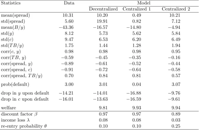
Table 1 presents statistics for the Argentina data and for the decentralized and centralized borrowing models. The first column shows business cycle statistics for Argentina from 1983 to 2001. The annual default probability of 3% is based on three default episodes in ap-proximately one hundred years. The average debt over GDP ratio of 43.36% is calculated for the period from 1983 to 2001 using Global Development Finance. The debt statistics include total external debt of the private and public sectors. The second column of Table 1 presents the statistics in the model with decentralized borrowing. To highlight the role of decentralized borrowing, we present these statistics in the model with centralized borrowing under the same set of parameter values in the third column.
Table 1: Comparison of Decentralized and Centralized Borrowing
Statistics Data Model
Decentralized Centralized 1 Centralized 2
mean(spread) 10.31 10.20 0.49 10.21 std(spread) 5.60 19.91 0.82 7.12 mean(B/y) −43.36 −16.57 −14.80 −4.94 std(y) 8.12 5.73 5.62 5.84 std(c) 9.47 6.53 6.20 6.49 std(T B/y) 1.75 1.44 1.28 1.94 corr(c,y) 0.98 0.98 0.98 0.95 corr(T B,y) −0.59 −0.45 −0.35 −0.16 corr(spread,y) −0.89 −0.61 −0.52 −0.44 corr(spread,c) −0.91 −0.72 −0.64 −0.58 corr(spread,T B/y) 0.70 0.84 0.81 0.57 prob(default) 3.00 3.01 0.04 3.07
drop iny upon default −14.21 −14.01 −16.88 −9.76
drop inc upon default −16.01 −13.63 −16.59 −9.61
welfare 9.81 9.93 9.94
discount factor β 0.97 0.97 0.89
income lossλ 0.08 0.08 0.03
re-entry probability θ 0.10 0.10 0.25
Note: All statistics except correlations and welfare are in percentage terms. The income and consumption drops in default are based on the 2001 default episode. The interest rate spread is computed as the difference of the EMBI yield and the yield of a 5 year U.S. bond.
There are three striking differences between the decentralized and centralized borrowing models. First, the mean spread under decentralized borrowing is higher by a factor of more than twenty compared to that under centralized borrowing. Second, the model with decentralized borrowing exhibits a much higher default probability, 3.01%, far exceeding 0.04% in the model with centralized borrowing. Third, the decentralized borrowing model generates a higher debt to income ratio than the centralized borrowing model does. The mean debt to income ratio is 16.57% in the decentralized borrowing model, while it is 14.80% in the centralized borrowing model.
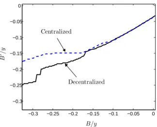
To understand these differences, we examine borrowing decisions in the two models. Figure 3 plots the desired borrowing conditional on not defaulting over the current bond holdings.16 Desired borrowing is similar across the two models for low levels of debt. As
the debt level increases, desired borrowing increases faster under decentralized borrowing. Under centralized borrowing, the government recognizes that the interest rate increases as an additional unit of debt is taken. Under decentralized borrowing, however, households do not take into account the interest rate effect of their borrowing and would like to overborrow. This negative externality becomes especially severe when current debt is large and the interest rate rises sharply with an additional unit of debt.
Figure 3: Comparison of Desired Borrowing
−0.3 −0.25 −0.2 −0.15 −0.1 −0.05 0 −0.3 −0.25 −0.2 −0.15 −0.1 −0.05 0 B/y B 0/y Decentralized Centralized
Borrowing and default are two instruments with which households affect their consump-tion path. Under centralized borrowing, the government, or equivalently the representative 16All figures in this subsection are based on the income shock, which is 5% below the mean. We observe
the same qualitative results for the other income shocks. Both the current and next-period bond holdings are normalized by the mean income shock.
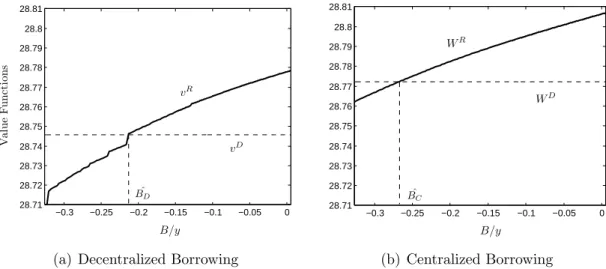
household, owns both instruments. Under decentralized borrowing, the households have only the first instrument and tend to take debt recklessly since they fail to internalize the negative externality of their borrowing. Thus, welfare, especially the repayment welfare, is lower under decentralized borrowing, as shown in Figure 4. Consequently, the government finds default attractive for a wider range of debt levels under decentralized borrowing.
Figure 4: Comparison of Value Functions
−0.3 −0.25 −0.2 −0.15 −0.1 −0.05 0 28.71 28.72 28.73 28.74 28.75 28.76 28.77 28.78 28.79 28.8 28.81 vR vD ˆ BD V al ue Fu nc ti on s B/y
(a) Decentralized Borrowing
−0.3 −0.25 −0.2 −0.15 −0.1 −0.05 0 28.71 28.72 28.73 28.74 28.75 28.76 28.77 28.78 28.79 28.8 28.81 WR WD ˆ BC B/y (b) Centralized Borrowing
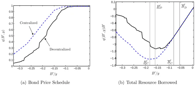
The failure of individual households to internalize the effect of their borrowing on the government’s default choices lowers the bond price schedule under decentralized borrowing. As shown in the left panel of Figure 5, the prices are discounted by more for any level of bonds under decentralized borrowing. This less favorable bond price schedule generates tighter debt limits and constrains borrowing by more. The right panel displays the total resources that debt generates, q(B0, y)B0. Any debt B0 less than the safe debt limit B0 generates resourcesB0/(1 +r). Once it exceeds the safe debt limit, the debt becomes risky. Let us refer to the debt level which maximizes the resource obtained from foreign lenders, q(B0, y)B0, as the risky debt limit, denoted by B0. The optimal level of debt would never exceed the risky debt limit because the borrower can obtain the same amount of resources with a smaller next-period repayment. As shown in the figure, both the safe and risky debt limits are tighter under decentralized borrowing.
The incentive to overborrow and the steeper bond price schedule have opposite effects on the equilibrium level of debt. Whether decentralized borrowing leads to larger equilib-rium debt depends on which force dominates. Under the benchmark calibration, desired borrowing is higher even when the bond price schedule is less favorable under decentralized borrowing. This leads to higher equilibrium debt under decentralized borrowing. Figure 6
Figure 5: Comparison of Bond Price Schedules −0.3 −0.25 −0.2 −0.15 −0.1 −0.05 0 0 0.1 0.2 0.3 0.4 0.5 0.6 0.7 0.8 0.9 1 B0/y q ( B 0,y ) Decentralized Centralized
(a) Bond Price Schedule
−0.3 −0.25 −0.2 −0.15 −0.1 −0.05 0 −1.6 −1.4 −1.2 −1 −0.8 −0.6 −0.4 −0.2 0 0.2 B0/y q ( B 0,y ) B 0 B0D B0D B0C B0C
(b) Total Resource Borrowed
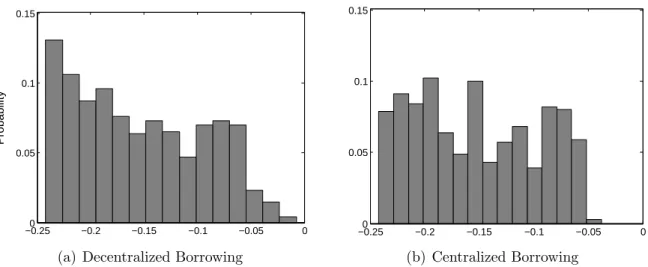
shows the limiting distribution of bond holdings as shares of mean income for the two mod-els. The distribution is more concentrated on high debt levels in the decentralized borrowing model, while it is more dispersed in the centralized borrowing model. This implies that even with higher costs of borrowing, the incentive to overborrow is strong enough to induce the households to issue more debt. As a result, the interest rate spread is substantially higher under decentralized borrowing. Also, the interest rate spread is more countercyclical under decentralized borrowing. As shown in Table 1, corr(spread, y) and corr(spread, c) are −0.61 and −0.72, respectively, under decentralized borrowing, and−0.52 and −0.64, respectively, under centralized borrowing.
Table 1 also reports the welfare statistics, measured as permanent consumption, for each simulated model.17 The welfare is 1% lower under decentralized borrowing than under
centralized borrowing. The 1% welfare difference is economically significant, considering that the welfare cost of business cycles estimated by Lucas (1987) is only about one-tenth of a percent of consumption.18
In summary, the decentralized borrowing model generates a larger default rate, a higher mean spread, lower welfare and larger equilibrium debt than the centralized borrowing model in the benchmark calibration. All these findings, except the one on equilibrium debt, are robust to different default penalty parameters and specifications. We will discuss these robustness checks in the next section.
17The welfare calculation is based on the limiting distribution.
Figure 6: Comparison of Bond Distributions −0.250 −0.2 −0.15 −0.1 −0.05 0 0.05 0.1 0.15 Probability
(a) Decentralized Borrowing
−0.250 −0.2 −0.15 −0.1 −0.05 0
0.05 0.1 0.15
(b) Centralized Borrowing
3.3
Quantitative Predictions of the Models
In this subsection, we compare the quantitative predictions of the two models with the Argentine data. Both models are calibrated to match the relevant moments in the data. In particular, the parametersβ, λ, andθ are calibrated to best match the default rate, income loss, and trade-balance volatility in the data. Unlike the model with decentralized borrowing, the model with centralized borrowing has difficulty in generating all three moments. To generate a realistic default probability, it needs an unrealistically low discount factor of 0.89, implying a quarterly interest rate as high as 12%. Under such a low discount factor, the volatility of the trade balance is high and the income loss during default is small relative to the data. The fourth column of Table 1 shows the statistics of the recalibrated model with centralized borrowing.
The most striking difference across these two models is the equilibrium debt level. The debt to income ratio is less than 5% in the model with centralized borrowing. However, it is about 17% in the model with decentralized borrowing—much closer to the data. The model with centralized borrowing can generate larger equilibrium debt, but only at the expense of substantially lowering equilibrium default rates. In contrast, the model with decentralized borrowing has an inherent mechanism to produce both aspects jointly: households tend to borrow more and the government tends to default more. Importantly, the decentralized borrowing model brings the key moments closer to the data without resorting to unrealistic discount factors.
The model with decentralized borrowing also shows better performance in terms of repli-cating countercyclical trade balances and interest rate spreads. The correlation between the trade balance and income is−0.59 in the data; it is only−0.16 in the model with centralized borrowing, but −0.45 in the model with decentralized borrowing. The correlation between the interest rate spread and income is−0.89 in the data; it is only −0.44 in the model with centralized borrowing, but −0.61 in the model with decentralized borrowing. Both mod-els replicate well the mean interest rate spread, the income volatility and the consumption volatility. In particular, consumption is more volatile than income. On the other hand, the model with decentralized borrowing overestimates the volatility of the interest spread.
4
Overborrowing or Underborrowing
The calibrated model with decentralized borrowing generates a larger default rate, a higher mean spread, lower welfare and larger equilibrium debt than the model with centralized bor-rowing. This section examines whether these results are robust to different default penalty parameters and to an alternative symmetric specification of the default penalty. We find un-der all variations that decentralized borrowing implies a larger default rate, a higher mean spread, and lower welfare. The overborrowing result, however, is not robust: the decentral-ized borrowing model might generate underborrowing as we vary the default penalties.
4.1
Alternative Default Penalty Parameters
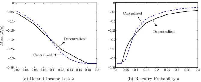
Consider the two models with the benchmark parameter values. In the first set of experi-ments, we vary the default income loss parameterλfrom 1% to 20% while fixing all the other parameters. In the second set of experiments, we vary the re-entry probability from 1% to 40% while fixing all the other parameters. We plot the equilibrium debt to income ratios of the two models for these two sets of experiments in Figure 7. First of all, equilibrium debt in both models increases with the default income lossλand decreases with the re-entry probability θ. This is intuitive because larger values of λ or lower values of θ are associated with more severe default penalties, and this in turn implies less frequent default and more lenient bond price schedules.
Second, we find that decentralized borrowing generates overborrowing for low values of λ, but underborrowing for high values of λ, as shown in the left panel of Figure 7. The differences in equilibrium debt appear to be small in the figure, but the magnitudes of overborrowing or underborrowing are not trivial. For example, decentralized borrowing
Figure 7: Equilibrium Debt: Varying Default Penalties 0.02 0.04 0.06 0.08 0.1 0.12 0.14 0.16 0.18 0.2 −0.35 −0.3 −0.25 −0.2 −0.15 −0.1 −0.05 0 M ea n ( B /y ) Decentralized Centralized
(a) Default Income Lossλ
0 0.05 0.1 0.15 0.2 0.25 0.3 0.35 0.4 −0.35 −0.3 −0.25 −0.2 −0.15 −0.1 −0.05 0 Decentralized Centralized (b) Re-entry Probabilityθ
generates overborrowing by 19.9% when λ is 0.04 and underborrowing by 7.5% when λ is 0.12. Note that for λ higher than 0.18, no default happens and thus the equilibrium debt levels are identical in both models.
As we discussed earlier, decentralized borrowing has two conflicting effects on equilibrium debt: the overborrowing and bond price schedule effects. The overborrowing incentive arises from the failure of individual households to internalize the effect of their borrowing on the bond price. This overborrowing effect is strong when the bond price schedule is steep, which can be seen from comparing the first order conditions in equation (9) and (10). On the other hand, the bond price schedule effect arises from the failure of individual households to internalize the effect of their borrowing on the government’s default choices. This bond price schedule effect is strong when the difference between the bond price schedules in the two models is large.
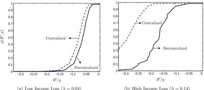
When λ is low, the bond price schedules in both models are steep and the difference between them is small, as shown in the left panel of Figure 8. This implies a strong overbor-rowing effect and a weak bond price schedule effect. Asλincreases, the bond price schedules in both models become flatter and the difference between them becomes larger, as shown in the right panel of Figure 8. This implies that the overborrowing effect weakens and the bond price schedule effect strengthens. Therefore, the overborrowing effect tends to dominate for low λ, but the bond price schedule effect tends to dominate for high λ.
Finally, we compare equilibrium debt of the two models for different re-entry probabilities
Figure 8: Bond Prices for Different Income Losses −0.3 −0.25 −0.2 −0.15 −0.1 −0.05 0 0 0.1 0.2 0.3 0.4 0.5 0.6 0.7 0.8 0.9 1 q ( B 0,y ) B0/y Decentralized Centralized
(a) Low Income Loss (λ= 0.04)
−0.3 −0.25 −0.2 −0.15 −0.1 −0.05 0 0 0.1 0.2 0.3 0.4 0.5 0.6 0.7 0.8 0.9 1 B0/y Decentralized Centralized
(b) High Income Loss (λ= 0.14)
when θ is low. In particular, equilibrium debt under decentralized borrowing is 47.5% more when θ is 0.3, but 14.5% less when θ is 0.07. The equilibrium debt levels are identical across the two models for very low values of θ, which implies no default in equilibrium. The intuition for these results is similar to that for different λ. When θ is high, the bond price schedules are steep and similar in both models, which leads to equilibrium overborrowing. When θ is low, the bond price schedules become flatter and the difference between them becomes larger, implying equilibrium underborrowing.
When the default rates are zero in both models, the two models generate identical business cycle statistics including the mean spread, default rate and welfare. In all the other cases, the model with decentralized borrowing generates larger default rates, higher mean spreads, and lower welfare than the model with centralized borrowing. Even when decentralized borrowing generates equilibrium underborrowing, the substantial difference in the bond price schedule, as shown in the right panel of figure 8, is enough to make the spreads higher in equilibrium. We report the detailed statistics for these experiments in Appendix B.
4.2
Alternative Default Penalty Specification
We now investigate the symmetric default penalty of the following form:
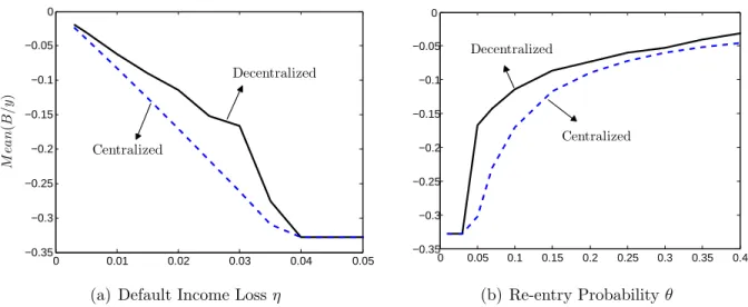
where η captures the constant fraction of income loss after default. Figure 9 shows equilib-rium debt levels for different values of η and θ. Surprisingly, under the symmetric default penalty, decentralized borrowing consistently generates underborrowing.
Figure 9: Equilibrium Debt under Symmetric Default Penalty
0 0.01 0.02 0.03 0.04 0.05 −0.35 −0.3 −0.25 −0.2 −0.15 −0.1 −0.05 0 M ea n ( B /y ) Decentralized Centralized
(a) Default Income Lossη
0 0.05 0.1 0.15 0.2 0.25 0.3 0.35 0.4 −0.35 −0.3 −0.25 −0.2 −0.15 −0.1 −0.05 0 Decentralized Centralized (b) Re-entry Probabilityθ
To understand this result, we plot the bond price schedules for both models under the symmetric default penalty in the left panel of Figure 10. In the right panel, we plot the resources obtained from foreign lenders, q(B0, y)B0, as a function of next-period debt. The bond price schedules are extremely steep and the risky-debt region [B0, B0] is tiny in both models. For the overborrowing effect to operate, the risky debt region needs to be large to accommodate the overborrowing incentives. Given the tiny risky debt region, equilibrium debt is mainly constrained by the safe debt limits in both models. Under decentralized bor-rowing, the overborrowing incentives tighten the safe debt limit greatly, and this translates into underborrowing in equilibrium.
As in the case with the asymmetric default penalty, the model with decentralized bor-rowing generates a higher default probability, a higher mean spread, and lower welfare for all the cases with positive default rates. We report the detailed statistics for different values of parameters in the symmetric default penalty case in Appendix B.
Our analysis shows that private borrowing does not necessarily lead to overborrowing when the lending practice is based on aggregate credit conditions. The shift from sovereign to private borrowing, however, unambiguously reduces welfare of domestic households and increases the likelihood of debt crisis. Therefore, regulations on private international borrow-ing are welfare improvborrow-ing. The most obvious policy would be to prohibit private borrowborrow-ing.
Figure 10: Bond Prices Under Symmetric Default Penalty −0.3 −0.25 −0.2 −0.15 −0.1 −0.05 0 0 0.1 0.2 0.3 0.4 0.5 0.6 0.7 0.8 0.9 1 q ( B 0,y ) B0/y Decentralized Centralized
(a) Bond Price Schedule
−0.3 −0.25 −0.2 −0.15 −0.1 −0.05 0 −1.8 −1.6 −1.4 −1.2 −1 −0.8 −0.6 −0.4 −0.2 0 0.2 B0/y q ( B 0,y ) B 0 B0D B0D B0C B0C
(b) Total Resource Borrowed
This would require that the government be able to efficiently allocate funds among house-holds. Alternatively, the government can impose, on international private borrowing, either taxes if there is overborrowing in equilibrium or subsidies if there is underborrowing in equi-librium.19 Future research on the optimal tax or subsidy on international private borrowing
will be useful since in practice it is hard to implement capital controls.
5
Conclusion
This paper presented a quantitative model of a small open economy with decentralized borrowing and centralized default. In the model, individual households make borrowing decisions and a government makes default decisions to maximize the welfare of the represen-tative household. Accordingly, foreign lenders price debt contracts based on macroeconomic variables: aggregate income shocks and aggregate debt levels. Private agents do not inter-nalize the negative externality of their borrowing on aggregate credit costs, and thus have incentives to overborrow. As a result, decentralized borrowing drives up the economy-wide credit costs, raises the likelihood of sovereign default, and lowers welfare.
Despite the overborrowing incentives, the model with decentralized borrowing does not necessarily lead to a higher level of equilibrium debt than the model with centralized bor-rowing. This is because households also face a less favorable bond price schedule under 19For discussions of optimal policy under complete markets, see Jeske (2006), Kehoe and Perri (2004) and
decentralized borrowing, which tends to reduce the optimal level of debt. When the in-come loss after default is disproportionately large under good inin-come shocks, decentralized borrowing generates overborrowing in equilibrium for lenient default penalties, but under-borrowing for severe default penalties. When the income loss is proportional to the income shock, decentralized borrowing always generates a lower equilibrium debt level for a wide range of default penalties.
The introduction of decentralized borrowing improves the quantitative fit of the model to the data. The standard sovereign debt models with centralized borrowing have difficul-ties in simultaneously generating a reasonable default rate and equilibrium debt level. In contrast, the model with decentralized borrowing has an inherent mechanism to improve the performance on both statistics jointly: the households tend to borrow more and the government tends to default more. Importantly, the decentralized borrowing model brings the key moments closer to the data without resorting to unrealistic discount factors.
References
Aguiar, Mark and Gita Gopinath, “Defaultable Debt, Interest Rates, and the Current Account,”Journal of International Economics, June 2006, 69 (1), 64–83.
Arellano, Cristina, “Default Risk and Income Fluctuations in Emerging Economies,”
American Economic Review, June 2008,98 (3), 690–712.
Bai, Yan and Jing Zhang, “Financial Integration and International Risk Sharing,”
Work-ing Paper, 2009.
and , “Solving the Feldstein-Horioka Puzzle with Financial Frictions,” Econometrica
(forthcoming), 2010.
Broner, Fernando and Jaume Ventura, “Globalization and Risk Sharing,” Review of
Economic Studies (forthcoming), 2010.
Cuadra, Gabriel and Horacio Sapriza, “Sovereign Default, Interest Rates and Political Uncertainty in Emerging Markets,”Journal of International Economics, 2008, 76, 78–88.
Eaton, Jonathan and Mark Gersovitz, “Debt with Potential Repudiation: Theoretical and Empirical Analysis,”Review of Economic Studies, April 1981, 48(2), 289–309.
Fernandez-Arias, Eduardo and Davide Lombardo, “Private External Overborrowing in Undistorted Economies: Market Failure and Optimal Policy,”Inter-American
Develop-ment Bank Working Paper Series 369, 1998.
Ferri, G., L.-G. Liu, and J. E. Stiglitz, “The Procyclical Role of Rating Agencies: Evidence from the East Asian Crisis,”Economic Notes, 1999, 28 (3), 335–355.
Gelos, R. Gaston, Ratna Sahay, and Guido Sandleris, “Sovereign Borrowing by Developing Countries: What Determines Market Access?,”Working Paper, 2008.
Greenwald, Bruce C. and Joseph E. Stiglitz, “Externalities in Economies with Imper-fect Information and Incomplete Markets,” Quarterly Journal of Economics, May 1986,
101(2), 229–264.
Hatchondo, Juan Carlos, Leonardo Martinez, and Horacio Sapriza, “On the Cycli-cality of the Interest Rate in Emerging Economy Models: Solution Methods Matter,”
Jeske, Karsten, “Private International Debt with Risk of Repudiation,”Journal of Political
Economy, June 2006, 114 (3), 576–593.
Kehoe, Patrick J. and Fabrizio Perri, “Competitive Equilibrium with limited enforce-ment,” Journal of Economic Theory, 2004, 119 (1), 184–206.
Levchenko, Andrei, “Financial Liberalization and Consumption Volatility in Developing Countries,” IMF Staff Papers, 2005, 52:2, 237–259.
Loong, Lee Hsien and Richard Zeckhauser, “Pecuniary Externalities Do Matter When Contingent Claims Markets Are Incomplete,”Quarterly Journal of Economics, Feb. 1982,
97(1), 171–179.
Lucas, Robert E. Jr., Models of Business Cycles, Oxford: Basil Blackwell, 1987.
Mendoza, Enrique G. and Vivian Z. Yue, “A Solution to the Default Risk-Business Cycle Disconnect,”NBER Working Papers 13861, 2008.
Otrok, Christopher, “On Measuring the Welfare Cost of Business Cycles,” Journal of
Monetary Economics, 2001, 47, 61–92.
Tauchen, George and Robert Hussey, “Quadrature-Based Methods for Obtaining Ap-proximate Solutions to Nonlinear Asset Pricing Models,” Econometrica, 1991, 59 (2), 371–396.
Uribe, Martin, “On Overborrowing,”American Economic Review, Papers and Proceedings, May 2006, 96 (2), 417–421.
Wright, Mark L.J., “Private Capital Flows, Capital Controls and Default Risk,” Journal
of International Economics, June 2006,69 (1), 120–149.
Yue, Vivian, “Sovereign Default and Debt Renegotiation,” Journal of International
Appendix A – Computational Algorithm
In this appendix, we describe the computation algorithm for each model. We start with the model with decentralized borrowing. We first discretize the state space (b, y, B0). We next make initial guesses for the bond price schedule and the government default decision. Specifically, we assume that q0(B0, y) = 1+1r for all (B0, y) and d0(B, y) = 0 for all (B, y). Given these guesses, we solve the individual household’s optimal debt level b0(b, y, B0), to-gether with the law of motion of aggregate debt B0 = Γ(B, y). Specifically, we accomplish this using the following steps.
We guess an initial law of motion of aggregate debt Γ0(B, y). We then solve for the
optimal value functions vR and vD and the optimal debt policy b0 using value function
iteration. We then smooth the continuation value in equation (3) over B0 by taking moving averages to minimize the spurious non-monotonicity in the optimal choices b0 overB0 due to discrete space methods. We update the law of motion of aggregate debt Γ1(B, y) such that
b0(b, y, B0) = B0. We iterate these procedures until Γ(B, y) converges. If there exist more than one fixed point, we take theB0 that gives the smallest debt.
We now update the default decision d1(B, y) by solving the government’s problem in equation (1). Accordingly, we update the bond price schedule. In order to minimize spurious movements in the bond price, we interpolate the bond price schedule. To do so, we first interpolate the value functions vR and vD over the income shock y. We next find an income
level ˆy(B) at whichvR(B,y(B), Bˆ 0) = vD(ˆy(B)) for each B. Note that ˆy(B) is not restricted
to the discrete shock levels. We then update q1(B0, y) = (1−Rˆy(B)
−∞ f(y
0|y)dy0)/(1 +r). We
iterate over the bond price schedule until it converges.
The computation algorithm for the model with centralized borrowing is simpler. We dis-cretize the state space (B, y). We start with a guess for the bond price schedule, q0
C(B
0, y) =
1
1+r for all (B
0, y). We next solve the optimal value functions WR, WD and the optimal
policy functionB0 using value function iteration. We then update the default decision based on WR and WD. We finally update the bond price schedule using a smoothing method analogous to that described above. We repeat the above procedures until the bond price schedule converges.
To see the effect of the bond price interpolation, Figure 11 shows the bond price schedule before and after the interpolation for the model with centralized borrowing. The discrete state-space (DSS) technique causes discrete jumps in the bond price, while our interpolation method removes spurious movements in the bond price. Simulation results show that the
interpolation greatly reduces the volatility and countercyclicality of the interest rate spread. Also, it reduces the default rate substantially, which suggests that the DSS method might overestimate the default likelihood.
Figure 11: Bond Price Schedule with and without Interpolation
−0.3 −0.25 −0.2 −0.15 −0.1 −0.05 0 0 0.1 0.2 0.3 0.4 0.5 0.6 0.7 0.8 0.9 1 B0/y qC ( B 0,y ) DSS DSS with interpolation
Note: The displayed bond price schedule is for an income shock 10% below the mean. The bond price schedules for other income shocks look similar.
Appendix B – Sensitivity Analysis
In this appendix, we report the simulation results for different default penalties. Table 2 presents the relevant statistics for the two models under the asymmetric default penalty specification for different values of default penalty parameters. The results can be summa-rized as follows. First, the decentralized borrowing model generates overborrowing when default penalties are lenient (corresponding to lowλ and highθ), and underborrowing when default penalties are severe (corresponding to high λ and low θ). Second, under all default penalty parameter values, the model with decentralized borrowing generates substantially higher mean spreads, larger default rates and lower welfare than the model with centralized borrowing.
Table 2: Varying Default Penalties: Asymmetric Income Loss λ θ 0.04 0.06 0.12 0.16 0.07 0.15 0.2 0.3 Decentralized mean(B/y) -8.44 -11.69 -25.13 -30.42 -20.79 -10.94 -8.44 -5.43 mean(spread) 12.04 10.35 9.79 9.29 10.15 10.40 11.53 14.06 prob(default) 3.88 3.30 2.62 2.13 2.93 3.49 4.23 5.13 welfare 9.73 9.73 9.83 9.72 9.77 9.74 9.73 9.75 Centralized mean(B/y) -7.04 -10.44 -27.01 -32.41 -23.80 -8.88 -6.15 -3.68 mean(spread) 0.44 0.43 0.29 0.05 0.28 0.68 0.84 1.31 prob(default) 0.08 0.05 0.07 0.00 0.05 0.06 0.13 0.37 welfare 9.94 9.93 9.89 9.83 9.91 9.92 9.92 9.93
Table 3 shows the simulation results for the symmetric default penalty specification. Unlike the asymmetric default penalty, independent of the default penalty parameter values, the decentralized borrowing model consistently generates lower equilibrium debt, higher mean spreads, higher default rates, and lower welfare.
Table 3: Varying Default Penalties: Symmetric Income Loss
η θ 0.005 0.015 0.02 0.03 0.05 0.1 0.15 0.35 Decentralized mean(B/y) -3.01 -8.99 -11.41 -16.68 -16.75 -11.41 -8.68 -4.01 mean(spread) 2.33 1.97 1.20 0.99 1.34 1.20 1.12 0.83 prob(default) 0.15 0.11 0.02 0.00 0.06 0.02 0.00 0.00 welfare 9.84 9.84 9.82 9.78 9.82 9.82 9.76 9.83 Centralized mean(B/y) -3.98 -12.55 -16.99 -26.18 -30.28 -16.99 -11.76 -5.18 mean(spread) 0.02 0.01 0.02 0.01 0.01 0.02 0.01 0.03 prob(default) 0.00 0.00 0.00 0.00 0.00 0.00 0.00 0.00 welfare 9.96 9.94 9.93 9.91 9.92 9.93 9.95 9.99