Differentially Private Learning with Noisy Labels

(1)

Differentially Private Learning with

Noisy Labels

by

Shubhanakar Mohapatra

A thesis

presented to the University of Waterloo in fulfillment of the

thesis requirement for the degree of Master of Mathematics

in

Computer Science

Waterloo, Ontario, Canada, 2020

c

(2)

Author’s Declaration

I hereby declare that I am the sole author of this thesis. This is a true copy of the thesis, including any required final revisions, as accepted by my examiners.

(3)

Abstract

Supervised machine learning tasks require large labelled datasets. However, obtaining such datasets is a difficult task and often leads to noisy labels due to human errors or adversarial perturbation. Recent studies have shown multiple methods to tackle this problem in the non-private scenario yet this remains an unsolved problem when the dataset is private. In this work, we aim to train a model on a sensitive dataset that contains noisy labels such that (i) the model has high test accuracy and (ii) the training process satisfies (, δ)-differential privacy. Noisy labels, as studied in our work, are generated by flipping labels in the training set, from the true source label(s) to other target(s). Our approach,_Diffindo, constructs a differentially private stochastic gradient descent algorithm which removes suspicious points based on their noisy gradients. We show experiments on datasets across multiple domains with different class balance properties. Our results show that the proposed algorithm can remove up to 100% of the points with noisy labels in the private scenario while restoring the precision of the targeted label and testing accuracy to its no-noise counterparts.

(4)

Acknowledgements

First of all, I would like to thank my supervisors for the immense support and time that they have given me throughout my research. Thank you, Prof. Helen Chen, for believing in me and for allowing me to be a research student with you. Thank you, Prof. Xi He, to introduce and help me learn this fascinating field of study and correct me whenever I went wrong. Both of your advice and support has led me to write this thesis today. I am incredibly fortunate to have been supervised by you and am excited about all our future endeavours. Thank you Prof. Florian Kerschbaum and Prof. Gautam Kamath for reading my thesis and for your comments on this work.

A huge thanks goes to Dr. Om Thakkar and Prof. Gautam Kamath(again) for guiding and collaborating towards the research for my thesis. I would also like to thank all the amazing researchers at the Data Systems group and WHISTL group at the University of Waterloo for all the lively and sometimes intricate discussions leading to the numerous ideas together. I’m fortunate to have met and have the chance to work with talented and hard-working researchers like you.

Thanks a million to all my amazing friends at UWaterloo who have spent hours with me at board games, badminton, Friday nights together at Uptown, planning get-togethers or have been to infinitely many coffee breaks and meanwhile always putting up with my atrocities and supporting me through the thick and thin. I also can’t go without thanking my friends back at home in India with whom I’ve had long video chats talking about life and end up absolutely going nowhere. I wish with all my heart that all our dreams come true.

Last but not least, I would like to thank my parents, Lilima Mohapatra and Santosh Mohapatra and my brother Soumyankar for the never-ending love and support. I would not be half the person that I am today if it wouldn’t be for you people. Your phone calls every morning motivated me to go through all the tough times. Love you Mamma, Papa and Chunnu!

(5)

Dedication

(6)

List of Tables

6.1 List of datasets . . . 30

6.2 Results on improvement of accuracy for _Diffindo ( = ∞) compare to SGD on MNIST . . . 33

6.3 Results on improvement of accuracy for _Diffindo ( = 3.6) compared to DPSGD (= 3.6) on MNIST . . . 33

6.4 Results on improvement of accuracy for _Diffindo ( = 4.98) compared to DPSGD (= 4.98) on ENRON . . . 35

6.5 Results on improvement of accuracy for _Diffindo ( = 5.44) compared to DPSGD (= 5.44) on APTOS . . . 37

6.6 Composite attack results for _Diffindo ( = 3.6) compared to DPSGD (= 3.6) . . . 39

6.7 Results on improvement of accuracy for _Diffindo (=∞) compare to SGD 41 6.8 Results on improvement of accuracy for _Diffindo ( = 3.3) compared to DPSGD (= 3.6) . . . 42

6.9 Performance of _Diffindo on varying noise levels . . . 43

6.10 Parameter study values . . . 44

(9)

List of Figures

3.1 Example of a label flip from Class 1 to Class 7 in MNIST . . . 15

4.1 Problem Setup . . . 18

6.1 _Diffindo has a higher precision than the baseline algorithms (DP-IMSAT and DPSGD). . . 32

6.2 Precision increase for target label (1) for _Diffindo on ENRON . . . 34

6.3 Performance of _Diffindo on medical dataset APTOS . . . 36

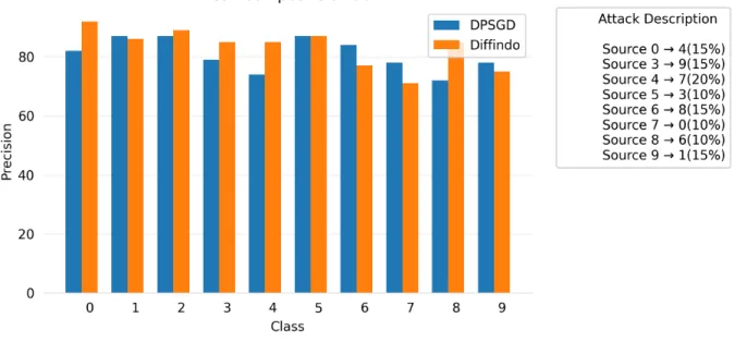
6.4 Precision comparison for all output classes on MNIST Tweak . . . 38

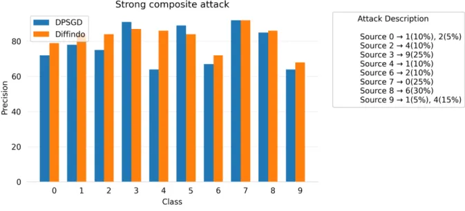
6.5 Precision comparison for all output classes on MNIST Tstrong . . . 39

6.6 CNN Model for _Diffindovs baseline algorithms (DP-IMSAT and DPSGD). 40 6.7 Comparison of _Diffindo vs DPSGD on varying noise . . . 43

6.8 Performance of _Diffindofor MNIST for varying one parameter, and others fixed at reference value . . . 46

6.9 Outlier points removal in _Diffindoat= 3.6and δ = 10−5 when ∆is 30%. 47 A.1 _Diffindo shows testing accuracy gains for the same privacy budget vs DPSGD over 48 attacks for each ∆ . . . 63

A.2 _Diffindo(=∞)shows testing accuracy gains vs SGD over 48 attacks for each ∆ . . . 64

(10)

Chapter 1 Introduction

The last decade has observed immense growth in deep learning. With the popularization of deep learning, the need for clean datasets has become of utmost importance, as the accuracy of the model is highly dependent on the quality of the training data [57,23]. One common data quality issue is noisy labels, which could arise due to several issues, including data entry errors [6], or data poisoning attacks [73], in which attackers inject fake points (e.g., creating fake accounts). If the model curator has direct access to the data as well as domain expertise, these noisy labels can be manually corrected or removed. However, cleaning these noisy labels is usually difficult, as many noisy datasets (e.g., medical data) are sensitive and private. One may be tempted to argue that the model curator could remove datapoints with manipulated labels from the training set by simply viewing the training point and manually adjusting the label. This is reasonable if the training points are interpretable, but is an impossible task if labelling requires significant domain expertise, or if there are a large number of outliers. The labelling of the points becomes an even harder task if the data is private and can not be directly accessed by the model curator. Motivated by these challenges, we investigate supervised learning with noisy labels in a private setting. There are numerous works in the literature focused on identifying and dealing with noisy labels in the non-private setting, but to the best of our knowledge, our paper is the first of its kind in the private setting.

Prior work in the non-private setting [60,57,61,39] have tried to learn with noisy labels using three methods. The first approach is to design models which are inherently robust to model flips. Researchers have achieved such models by building robust loss functions, adding extra layers in a neural network to remove noisy points or using some auxiallry knowledge. A second approach is to relabel the points using unsupervised clustering tech-niques. The idea is to cluster the points without using the labels (e.g., k-nearest

(11)

neigh-bours [61] or using validation from a separate set of trusted labels [28]), and then use the cluster centres to relabel points which are a minority in each cluster. The third approach instead is to identify and remove the label-flipped points from the training set [37, 13]. Diakonikolas, Kamath, Kane, Li, Steinhardt, and Stewart present a meta-algorithm called Sever[13] which is used on top of any stochastic optimization technique to remove outlier points based on scores calculated from the top most singular vector of variance of the gra-dients. They show experiments on traditional machine learning algorithms like SVM and logistic regression. However, none of these works consider private settings. In our work, we show that _Sever can be extended to neural networks and performs well on common machine learning datasets in the private scenario.

For quantifying our privacy guarantees, we consider the standard privacy notion, dif-ferential privacy (DP) [16]. It is the current gold standard of privacy and is being used by the US Census Bureau [50] and by many leading software industries like Google, Uber, Facebook and Apple [21, 80]. To make our learning model private, we use differentially private stochastic gradient descent (DPSGD) [83, 72, 5, 1], which can be an optimizer for any deep learning model. DPSGD is based on a stochastic optimizer which iteratively updates the parameters in the model to optimize the objective function. At each iteration, the empirical gradients are computed from a batch of sampled points and noise is added to the (clipped) gradients to ensure differential privacy. Applying the meta-algorithm _Sever to remove points in DPSGD is non-trivial, as there are several new issues that arise under the additional constraint of privacy. We address these issues and propose a new algorithm which is both private and robust.

The main contributions of our work are as follows :

• We are the first study to show that the accuracy of a differentially private machine learning algorithm is prone to noisy labels in the training data.

• We provide a novel differentially private algorithm for this setting of learning on noisy labels, named _Diffindo.

• Our results show that _Diffindo can remove an up to a 100% of the outliers and increase testing accuracy for upto the no-noise accuracy for baseline algorithms, in-cluding private unsupervised learning and DPSGD.

This thesis is organized as follows. We start by first looking into some prior related work specifically in DP machine learning and learning with noisy labels in the non-private scenario in Chapter 2. Next in Chapter 3, we describe some preliminary notations and fundamentals which would later help us in sketching out our algorithm and the problem

(12)

setup. As this problem has not been defined before in literature, we formally write down the problem setup and statement in Chapter 4. In Chapter 5, we introduce _Diffindo which is a method to remove outliers while training on private data. We extensively evaluate the proposed algorithm on multiple inputs across different datasets, models and label flips in Chapter 6. Finally, in Chapter 7, we conclude this thesis while discussing some open questions and future work in this field.

(13)

Chapter 2 Related Work

In this section, we look into the related work. We first start with differentially private machine learning, then move to literature work where researchers have presented machine learning algorithms to learn with noisy labels. Finally, we present background in health data where differentially private learning with noisy labels can be used.

2.1 Differentially Private Machine Learning

Simply anonymizing the dataset and scrapping off demographic and personal information does not provide privacy. This has been proven by multiple researchers in history. For example, in 2006, Narayanan and Shmatikov [55] showed that the adversary is able to re-identify the members of the Netflix dataset, which consisted of anonymized individuals and their choice of movies by extrapolating rankings and timestamps in IMDB public data repository. The same phenomenon was observed in other kinds of data like public health records [75], social network graphs [4], search query logs [31] and many more. In 2009, Wang et al. showed that releasing computed statistics from high-dimensional sensitive genetic data can also face the same fate of de-anonymization [82].

Similar data leakage trends have also been observed while training a machine learning model. There has been much previous work that has demonstrated this by showing different attack techniques to machine learning models. One such attack is a reconstruction attack, where the adversary tries to decode the training dataset by asking the model multiple statistical queries and getting them answered with certain accuracies [14, 22]. Another line of attacks is called themembership inference attack where the adversary tries to guess

(14)

whether a particular data point was used in the training of the machine learning model or not [29, 70, 7, 19, 71]. These attacks can even be made worse if the adversary has white box access to the machine learning model [56]. The third type of threat is focused onmemorization attacks, where it has been seen that a neural network has tendencies of memorizing sensitive information from training dataset [8].

These attacks led to research that tried to bound the training data information fed into the model by providing differential privacy guarantees. The US Census Bureau was the first big organization to adopt differential privacy in 2008 for a product called OnTheMap [50] and subsequently Google, Apple, Microsoft, Facebook and Uber followed [80]. Google used differential privacy to monitor and analyze the Chrome browser properties of its user base to detect security vulnerabilities [21]. Although some of the underlying differential privacy mechanisms such Laplace mechanism [17] and Gaussian Mechanism [15] can be used to compose into iterative machine learning tasks but it has been seen that they provide loose guarantees and lower utility. In recent years, differentially private machine learning has been a focus of many researchers and it has led to much work in this field. Differentially private empirical risk minimization using input, output and objective perturbation was first proposed by Choudhuri et al. in 2011 [9]. Later, a private stochastic gradient descent algorithm was proposed by Song et al. [72] and optimal risk bounds were provided later by Bassily et al. [5]. There have also been some works in the non-convex optimization setting including deep learning by Abadi et al. [1]. A broad and more in-depth analysis of DP machine learning algorithms can be found here [76]. Our problem aims to learn with the same differential private guarantees as prior work, but the prior work only considers clean data for training, but we use noisy (more specifically, label flipped) datasets for training.

2.2 Learning with Noisy Labels

Machine learning is highly dependent on the quality of data, and that is the reason why ML practitioners spend most of their time cleaning and preprocessing the data to get the best out of the models [23, 57]. Some studies have also shown that label noise can even be more impactful on the training process than feature noise itself [86, 65]. Noisy labels in the training data is a common problem in the medical field because obtaining clean and accurate medical data is a challenging task [43, 35]. Additionally, it is even a harder task to label this kind of data as expert domain expertise or consensus from a group of experienced doctors is required [62]. Getting hold of medical data becomes a herculean task when these problems are combined with stringent health and government standards and policies. Some studies have been able to successfully gather health data

(15)

by employing a large number of experts to annotate the datasets, but such efforts require massive financial and logistic resources [25]. Alternatively, a few studies have successfully used automated mining of medical image databases such as hospital picture archiving and communication systems (PACS) to build large training datasets [84]. However, this method is not always applicable, as historical data may not include all the desired labels or images. To mitigate the above issues, some studies have tried to collect data by crowd-sourcing them to get labels from non-experts. However, even for relatively simple segmentation tasks, computerized systems have been shown to generate significantly less accurate labels compared with human experts and crowd-sourced non-experts [27]. Given this scenario, it is becoming hard for deep learning practitioners to get hold noise-free datasets [10]. Hence, algorithmic solutions to get rid of noisy labels are highly desired in the medical field. In this section, we will discuss some prior work in learning with noisy labels with a focus on deep learning.

Researchers have tried to tackle noisy labels in multiple ways which can be broadly classified into the three following categories :

1. Design based methods - These methods aim at devising models that can inherently be robust to label noise. This can be achieved by altering the model, the loss function or the training procedure. Ghosh et al. studied the conditions for the robustness of a loss function to label noise for training deep learning models [24]. Two ways of improving the robustness of a loss function of deep learning models were proposed in Patrini et al. [60]. Several studies have proposed adding a “noise layer" to the end of deep learning models. The noise layer proposed by [74] is equivalent to mul-tiplication with the transition matrix between noisy and true labels. The authors developed methods for learning this matrix in parallel with the network weights us-ing error back-propagation. A similar noise layer was proposed by [77] for training a generative adversarial network (GAN) under label noise. Some papers have also tried a distillation approach based on the auxiliary knowledge learnt from some clean training data. The training starts by assigning a pseudo-label based on the con-vex combination of auxiliary knowledge and noisy label. They suggested that as the training proceeds, the model becomes more accurate, and its predictions can be weighed more strongly, thereby gradually forgetting the original incorrect labels. 2. Clustering based methods - Usually, the noisy labels are dominated by the correct

labels, and there is a considerable correlation between the correct labels which out-cast the noisy labels out. Authors have found high correlations in the latent space generated after some layers of a network. These correlations have shown clusters of the noisy labelled datapoints [44]. Another example is the work of [85], where the

(16)

authors proposed a method to leverage the multiplicity of data samples with the same (noisy) label in each training batch. All samples with the same label were fed into a light-weight neural network model that assigned a confidence weight to each sample based on the probability of it having the correct label. Some authors have tried data re-weighting techniques to down weight the datapoints, which have a high probability of having noisy labels [66]. A clean validation set is used to determine the weights assigned to the training data with noisy labels. The authors showed that this weighting scheme was equivalent to assigning larger weights to training data samples that were similar to the clean validation data in terms of both the learned features and optimization gradient directions.

3. Filtering methods - The methods in this bracket either try removing the points with the noisy labels or try de-noising them back to its original label. The filtering pro-cess can be applied before the training propro-cess as a pre-propro-cessing step or whilst training. An example of this method is [79], where authors propose supervised and unsupervised methods to obtain the correctly labelled images from a collection of images. CleanNet, proposed by [45], extracts a feature vector from a query image with a noisy label and compares it with a feature vector that is representative of its class. The representative feature vector for each class is computed from a small clean dataset. The similarity between these feature vectors is used to decide whether the label is correct. In [47], a teacher-student based learning is proposed in which the student learns on a noisy dataset and the teacher who has some prior knowledge on a clean dataset helps the student in learning. The student model was encouraged to be consistent with the teacher model using a meta-objective in the form of the KL divergence between prediction probabilities. A similar area of research is the robust mean estimation problem, which is applied to more classical machine learning tasks that go back to Tukey and his students [78]. Recently, there has been much work in this direction for mean and co-variance estimation [12,40, 63] leading to a meta-algorithm called _Sever which can be used on top of the gradient descent algorithm to remove data point with noisy labels(outliers) from the training dataset [13]. Here we have stated some of the previous work in this area and more related work can be found in [35]. Despite the numerous work in treating datasets with noisy labels for learning, there has been no advancement for doing the same in the private setting up to the best of our knowledge. This problem is well observed with medical data where access to health care data is plagued by vulnerability due to patient privacy considerations, which are protected by federal and local laws of protected health information such as the Health Insurance Portability and Accountability Act of 1996 (HIPAA). The fear of litigation and

(17)

breach of privacy discourages providers from sharing patient health data, even when they are de-identified [2]. Noisy labels and privacy issues have made medical data an important use case for differentially private learning with noisy labels.

In this paper, we build on the _Sever algorithm and use it in the private setting. One might be tempted to privatize any of the above algorithms, but the reason why we choose _Sever as our best candidate is threefold. Firstly, it can be directly applied to the gradients, and as DPSGD already sanitizes the gradients, _Sever is a comfortable fit. Secondly, _Sever has previously shown not only to remove label flipped points but also adversarially generated points. We study further on adversarial data poisoning for our proposed algorithm in Appendix A. Thirdly, _Sever provides theoretical guarantees for outlier point removal in higher dimensions while minimizing the loss function in the non-private scenario. This is beneficial while learning modern machine learning image datasets. We leverage these perks in our proposed algorithm.

(18)

Chapter 3 Preliminaries

In this section, we recall the definition of basic notions in machine learning, differential privacy, differentially private SGD, noisy labels, and the algorithm_Sever, a non-private algorithm to combat data poisoning which our private method is based on.

3.1 Machine Learning

A supervised learning task takes in a set ofn training points of the form(x1, y1), ..,(xn, yn),

where xi ∈ X is the feature vector of the ith point and yi ∈ Y is its label (or class). The

distribution of the random variables (X,Y) ∈ X × {1,2, . . . , C} is defined as D where the feature space is X ⊆ Rd _and _C _{is the number of classes. The goal is to train a}

parameterized function that takes in a feature vector x∈ X and outputs a label y∈ Y to fit the training data with respect to a loss function.

A loss function on parameters θ measures the difference between the labels predicted by θ-based function and the true labels in the training data. For example, the loss L(θ) onθ can be the average of the loss over the training points, i.e., L(θ) = 1

n

P

iL(θ, xi). The

learning task aims to minimize this loss function, but the loss function in complex models is usually non-convex and thus is difficult to minimize. Some common loss functions are the MSE (Mean Square Error) [46] which is mostly used for regression problems, Hinge Loss (used for SVMs) [69] and Cross Entropy loss [42] which is used for binary or multi class classification problems.

An optimizer like stochastic gradient descent (SGD) [67] is commonly used to reduce the loss function by iteratively updating the parametersθin the negative gradient direction. At

(19)

each iteration,t, a batch of pointsB from the training data is sampled and the gradient of the loss functiongtis estimated using these samplesB. The model parameters are updated

as θt+1 =θt−η·gt, where η is the learning rate. SGD is ubiquitous in practice and seems

to be effective at minimizing loss functions even in non-convex settings.

In our experiments, we use logistic regression and two common neural network architec-tures, a multi-layer perceptron and a convolutional neural network. Our logistic regression model is used on binary classification task and hence we use the Binary Cross Entropy loss and the neural networks are built for multi-label classification task and hence we use a variation of the cross entropy loss called the negative log-likelihood loss. However, the proposed algorithm in this thesis is not restricted to the aforementioned models and can be extended to any other models for supervised classification tasks.

3.2 Differential Privacy

Differential privacy (DP) [16, 17] is the gold standard privacy guarantee for learning pat-terns in the datasets to protect sensitive information of individuals. Formally, it is defined as follows.

Definition 1 (Differential Privacy). A randomized algorithm M : D → R with domain D and range R satisfies (, δ)-differential privacy (DP) if for any two adjacent inputs D, D0 ∈ D that differ in an entry and for any subset of outputs S ⊆ R it holds that :

Pr[M(D)∈ S]≤ePr[M(D0)∈ S] +δ

The original implementation of Differential Privacy does not include the additive term δ. We use the variant used in [15], which allows for the possibility that the vanilla -Differential Privacy can be broken with probability δ (which is ideally set to << _|D|1 ).

Differential Privacy has many advantages likepost-processing andadaptive composition which we define next.

Lemma 3.2.1 (Post-Processing [16]). If a mechanism M :D → R is (, δ)-differentially private, then for any function f :R → R0_{, we have that} _f_{◦ M} _{is also} _{(, δ)-differentially} private.

Lemma 3.2.2(Basic Composition [16]). For eachi∈[k], let algorithmMi :D × i−1

Y

j=1 Rj →

(20)

Ri be (i, δi)-DP in its first argument. If algorithm M[k]:D ×

k

Y

j=1

Rj is defined such that :

M[k]= (M1(D),M2(D,M1(D)),· · · ,Mk(D,M1(D)),· · · ,Mk−1(D)) thenM[k] is _Xk i=1 i, k X i=1 δi -differentially private.

Lemma 3.2.3 (Advanced Composition [34, 18]). For each i ∈ [k], let algorithm Mi :

D ×

i−1

Y

j=1

Rj → Ri be (i, δi)-DP in its first argument. If algorithm M[k] : D ×

k

Y

j=1 Rj is

defined such that :

M[k]= (M1(D),M2(D,M1(D)),· · · ,Mk(D,M1(D)),· · · ,Mk−1(D))

then for every δ0 >0, algorithm M[k] is (0,1−(1−δ0)

k Y i=1 (1−δi)) - DP, where 0 = min       k X i=1 i, k X i=1 i(ei −1) ei + 1 + v u u u u u u u t min     k X i=1 22_i log     e+ v u u t k X i=1 22_i δ0     , k X i=1 22_i log 1 δ0          

One of the classic DP algorithms is the Gaussian mechanism. To define the Gaussian mechanism, we will first describe the global sensitivity of a function.

Definition 2 (L2-sensitivity). A function f :D → R has L2-sensitivity Sf if

max

D,D0∈D

s.t(D,D0)neighbours

||f(D)−f(D0)||2 =Sf

Lemma 3.2.4(Gaussian Mechanism [17]). If a function f :D → R has L2-sensitivity Sf,

and a mechanism Mhas on inputD∈ D outputs f(D) +b, where b∼ N0, σ2_I

n×n), then

for c2 _>_{2 ln(1.25/δ), the mechanism} _M _{with parameter} _σ _≥ _cS

f/ is (ε, δ) -differentially

private. Here, N(0, σ2_I

n×n) denotes a vector of n i.i.d samples from the zero-mean

(21)

The analysis of this mechanism can be donepost hoc or during an iterative process to break if a certain threshold is met. Note that there are infinitely many(, δ)pairs satisfying this equation and to get a certain bound one of the values need to be fixed.

3.3 Differentially Private SGD

Complex DP algorithms can be built from the basic primitives based on post-processing and composition properties of DP. Usually, a differentially private additive noise mecha-nism consists of the following step: approximate the whole algorithm using the sequential composition of bounded-sensitivity functions; choosing appropriate noise parameters and finally performing the privacy analysis by a composition theorem to report the final pri-vacy cost. One of such algorithms is the Differentially Private Stochastic Gradient Descent (DPSGD). It is an approach inspired by the vanilla SGD to control the influence of any data point during the training process. The gradients of SGD are the random variables to which the noise is added. However, as there is no apriori bound of this gradient, the sensitivity Sf is calculated by clipping the maximum `2-norm to a user-defined parameter

called C. Algorithm 1 outlines our basic method for training a model with parameters θ by minimizing the empirical loss function L(θ). At each step of the SGD, we compute the gradient ∇θL(θt, xi) for a random subset of examples, clip the `2 norm of each gradient

to a maximum clipping factor of C, compute the average, add Gaussian noise with mean 0 and variance of bounded sensitivity C multiplied with the noise multiplier σ to protect privacy, and take a step in the opposite direction of this average noisy gradient. In the end, in addition to outputting the model, we will also need to compute the privacy loss of the mechanism based on the information maintained by the privacy accountant also known as the Moments Accountant.

We follow these steps while designing our algorithm in Chapter5. We use the Moments Accountant described in [1] for privacy accounting. The details of the Moments Accountant is described below.

Moments Accountant

The moments accountant based on Rényi-DP [53] keeps track of a bound on the mo-ments of the privacy loss random variable (In our case, gradients). It generalizes the standard approach of tracking (, δ) and using the strong composition theorem. While such an improvement was known previously for composing Gaussian mechanisms, it ap-plies also for composing Gaussian mechanisms with random sampling and can provide a much tighter estimate of the privacy loss iterative processes like gradient descent. It is

(22)

Algorithm 1: DPSGD

Data: Training set A:{x1, ...xn}, Loss function L(θ), Parameters: Learning rate

η, Lot size L, Gradient norm boundC Noise scaleσ, Total number of iterations T

Result: Model with trained parameter θ

1 Initialize model with θ₀ randomly; 2 for t∈[1, T]do

3 Sample a random subsetL_t ⊆A, by independently including each element of A

with probabilityL/n ;

4 for i∈Ab do

5 Compute gradient g_t(x_i) = ∇_θL(θ_t, x_i);

6 Clip each gradient in`₂ norm to C: ¯g_t(x_i) = g_t(x_i)/max(1,kgt(_Cxi)k2);

7 end

8 Add noise ˜gt = _|_L1_|(P_ig¯t(xi) +N(0, σ2C2I));

9 Gradient descent θt+1 =θt−η˜gt;

10 end

11 returnθ_T and compute the overall privacy cost (, δ)

difficult to use advanced composition for iterative mechanism like DPSGD as each appli-cation of an advanced composition theorem leads to a wide selection of possibilities for (, δ)-differentially private guarantees.

Privacy loss is a random variable dependent on the random noise added to algorithm1. That a mechanism M is (, δ)-differentially private is equivalent to a certain tail bound on M’s privacy loss random variable. While the tail bound is very useful information on a distribution, composing directly from it can result in quite loose bounds. Moments Accountant instead computes the log moments of the privacy loss random variable, which composes linearly. Then it uses the moments bound, together with the standard Markov inequality, to obtain the tail bound, that is the privacy loss in the sense of differential privacy. More specifically, for neighbouring databasesDandD0_{, a mechanism}_{M, auxiliary} input aux, and an outcomeo ∈ R, define privacy loss as

c(o;M,aux, d, d0)_,log P r[M(aux, d) = 0]

P r[M(aux, d0_{) = 0]} (3.1) A common design pattern, which is used extensively in the paper, is to update the state by sequentially applying differentially private mechanisms. This is an instance of adaptive

(23)

composition, which we model by letting the auxiliary input of thekth _mechanism _M k be

the output of all the previous mechanisms.

For a given mechanism M, we define the λth _moment _αM(λ;_aux_{, d, d}0₎ _{as the log of} moment generating function evaluated at the value of λ:

αM(λ;aux, d, d0)_,log_Eo∼M(aux,D)[eλc(o;M,aux,d,d 0₎

] (3.2)

In order to prove privacy guarantees of a mechanism, it is useful to bound all possible αM(λ;aux, d, d0). We define

αM(λ)_, max

aux,d,d0αM(λ;aux, d, d 0

)

where the maximum is taken over all the possibleaux and all neighbouring datasetsD,D0_. We state the properties of α that we use for Moments Accountant.

Theorem 3.3.1. Let αM be defined as above. Then,

1. [Composability] Suppose that a mechanism M consists of a sequence of adaptive mechanisms M1,· · · ,Mk where Mi :Qi

−1

j=1Rj× D → Ri. Then, for any λ

αM(λ)≤

k

X

i=1

αM_i(λ)

2. [Tail Bound] For any >0, the mechanism M is (, δ)-differentially private for δ = min

λ e

αM(λ)−λ

The proof to the theorem is given in [1]. By Theorem 3.3.1 it suffices to compute, or bound,αM(λ)at each step and sum them to bound the moments of the mechanism overall. We can then use the tail bound to convert the moments bound to the (, δ)-differential privacy guarantee.

(24)

3.4 Noisy Labels

Training data collected from unreliable sources usually have noisy labels. This noise can range from being identically split into different target labels (non-adversarial and natural noise) to skewed label flips (adversarially perturbed noise). Deep neural networks have been found to be naturally robust to label flips when larger networks and batch sizes are used [68]. In their work, the dataset of size n is diluted by adding ∆n points with flipped labels, where ∆ is the noise level. This does not change the available number of original examples and the original distribution is preserved.

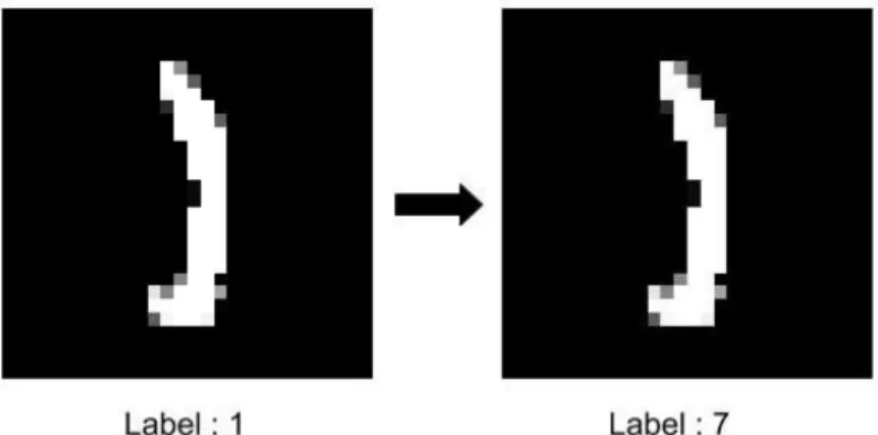
Figure 3.1: Example of a label flip from Class 1 to Class 7 in MNIST

In our work, we consider a stronger label flipping attack. Instead of adding noisy points, we use a transition matrix to change fraction of existing data points of one class to a target class [74]. We empirically show that this kind of attack not only degrades the test accuracy of the model but drastically reduces the precision of the target class. In other words, examples drawn from distribution D is unavailable and instead what we observe are noisy training samples {(x1,y1), . . . ,ˆ (xn,yˆn)}, where xi ∈ X and yˆi denotes the noisy

labels. We call this new noisy distribution Dˆ and it has the same feature and label space (X,Y)ˆ ∈ X ×1,2, . . . , C .

Transition Matrix : The random variables Yˆ and Y are related through a transition matrix also known as acorruption matrix T ∈[0,1]C×C. Each element of this matrixTi,j

stores the probability of elements from source class ito target class j. Ti,j =p(ˆy=j|y=i)

(25)

Such matrices can help us in modelling single-targeted as well as composite label noises. When running our experiments, we implement this noisy flips by getting all the indices of the source class and randomly changing the labels of these source points to the target labels as given in the transition matrix. We also denote the total percentage of labelled flipped as ∆. In other words, this is the total sum of all the elements in the transition matrix.

3.5 _Sever

Sever [13] is a meta-algorithm to filter outlier points based on their gradients in the training process. Outliers, as defined by Diakonikolas et al. can be mislabelled points defined just like the section above or adversarially added fake points to the training dataset. In their paper, they show that even a small fraction of these outliers in the training set can drastically affect the testing error of traditional machine learning algorithms like SVM and logistic regression. This algorithm takes in a batch of points, projects their gradients onto a carefully chosen direction, and removes a fraction of points with large projected values. _Sever possesses strong theoretical guarantees and it has been shown to achieve positive results on corrupted datasets and traditional machine learning models like ridge regression and support vector machines. Unlike many other filtering based noisy label removal algorithms,_Severhas no dependence on the underlying dimension of the training set d and hence, have better robustness in higher dimensions. Our work is the first time that _Severis being used for neural network models.

Now, we show one of the important theorems from _Sever which is used to build the proposed algorithm in this thesis. We start by defining γ-approximate critical point. Definition 3 (γ-approximate critical point). Given a function f :D → R, γ-approximate critical point of f, is a pointw∈ D so that for all the unit vectors v where w+δv∈ D for arbitrarily small positive δ, we have that v· ∇f(w)≥ −γ.

Essentially, the above definition means that the value of f cannot be decreased much by changing the input w locally while staying within the domain. The condition enforces that moving in any direction v either cause us to leaveD or causes f to decrease at a rate at most γ.

(26)

Definition 4 (γ-approximate learner). A learning algorithm L is calledγ-approximate if, for any functionsf1,· · · , fn :D → R each bounded below on a closed domainD, the output

w=L(f1:n) of L is a γ-approximate critical point of f(x) := 1_n n

X

i=1 fi(x).

In other words, L always finds an approximate critical point of the empirical learning objective. We note that most common learning algorithms (such as stochastic gradient descent) satisfy theγ-approximate learner property. We are now ready to present Theorem 2.1 from [13] which shows that the algorithm _Sever always finds a γ-critical point with high probability.

Theorem 3.5.1. Suppose that functions f1,· · · , fn:D → Rare bounded below on a closed

domain D, and suppose that they satisfy the following deterministic regularity conditions: There exists a set Igood ⊆[n] with |Igood| ≥(1−∆)n and σ >0 such that:

1. CovIgood[∇fi(w)]σ

2_{I, w}_{∈ D,} 2. ||∇fˆ(w)−f¯(w)||2 ≤σ

√

∆, w ∈ D, where fˆdef= (1/|Igood)

P

i∈Igoodfi .

Then the algorithm _Sever applied to f1,· · · , fn,∆ returns a point w ∈ D that, with

probability at least 9/10 is a (γ+O(σ√∆))- critical point of f.ˆ

Note that there is no dependence of the dimensiond and hence enabling_Severto per-form well on higher dimensional data (e.g. Image data). We built our proposed algorithm on top of this Theorem making it suitable in the private scenario.

(27)

Chapter 4 Problem Setup

To the best of our knowledge, there have been no previous work in private learning with noisy labels and therefore, in this chapter, we formally define the problem statement and setup.

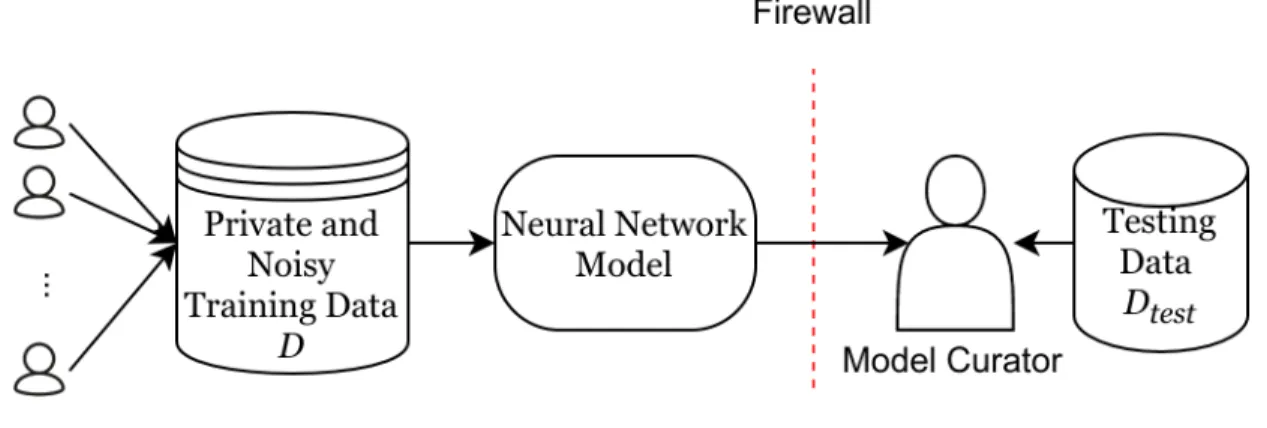
Figure 4.1: Problem Setup

Consider a set of sensitive and noisy training dataD which is a set ofntraining points of the form{(x1, y1), . . . ,(xn, yn)}, where xi ∈ X is the feature vector of theith point and

yi ∈ Y is its label (or class) collected from users and sitting on a server behind a privacy

firewall as shown in Figure 4.1. A model curator resides on the other side of the firewall and has no direct access to the dataset. However, a differentially private learning algorithm is allowed to run on the private dataset, and the learned model can be shared with the model curator. The curator is also not aware of any corruptions made to the data, but the curator has a set of clean testing data Dtest with correct labels which can be used to test

(28)

the final accuracy of the model. Also, note that the corruptions in the data (which in our case is generated by the transition matrix) can be targeted towards a specific class or set of classes. In such cases, we would also like to ensure high precision for the affected classes with the overall testing accuracy onDtest.

Problem Statement: Given a training datasetDwith noisy labels, we would like to train a neural network model on D such that (i) the training process satisfies (, δ)-differential privacy, and (ii) the model predicts the labels of the points in the testing dataset Dtest

with high accuracy. In particular, if many training points are mislabeled to certain target class(es), the learned model may misclassify many testing examples to such class(es) re-sulting in low precision value(s). Hence, we would like to ensure high precision per class in the testing data.

(29)

Chapter 5 Our Approach

5.1 Overview

In this section, we outline the non-private method upon which our approach is based, highlight some new challenges which arise in our setting and summarize the modifications necessary to overcome these challenges.

Our approach is based on the non-private algorithm _Sever [13], which can be briefly described as follows. Given some learning task, a model is first trained (ignoring any corruptions present in the data) to a local optimum. For instance, this could simply involve optimizing the parameters of the model (in order to minimize the loss function) using SGD, but any other appropriate optimization method could also be used as a black box. Given this optimum, the following “filtering” algorithm is run: we compute the empirical gradients of the training set, take the covariance matrix of these gradients, find the top eigenvector direction, and remove points whose gradient when projected onto this direction is too large. We repeat the entire procedure on the pruned dataset until convergence. An appropriate instantiation of this framework has strong provable guarantees, and [13] also demonstrates that it is effective in practice for simple models, including logistic regression and support vector machines (SVMs).

However, in the setting we are concerned with, there are a number of new considerations that arise. Most obvious is the constraint of differential privacy, but thescaleof the datasets and models we investigate also have their own associated problems.

To elaborate on the last point, the largest dataset and model considered in [13] is the Enron dataset [51] trained on a SVM model, and thus the problem as a whole has roughly

(30)

4,000 training points and 5,000 parameters. In comparison, since one of our datasets and models is the MNIST dataset [41] on a multilayer perceptron, the problem has 60,000 training points and nearly 800,000 parameters – overall, several orders of magnitude larger! As it would be impractical to store data of this scale in memory (e.g., the covariance matrix alone would have 8000002 ≈7×1011 entries), we are forced to turn to other options. Our method instead performs filtering using the gradients with respect to only the input pixels (rather than the parameters of the model), reducing the dimensionality from 800,000 to roughly800.

Turning to issues that arise due to privacy: in a differentially private setting, it is not cheap to train a model to optimality using DPSGD, as _Sever would prescribe. In particular, each privatized step of SGD will expend a fraction of our privacy budget, and we must be judicious with our choice of how many steps to take before running the filtering procedure.

More broadly speaking, there are many steps in the framework which must be priva-tized. The choice of how to split up our privacy budget (as well as the associated hyperpa-rameters) gives rise to many important design decisions. In addition to the standard noise injection in DPSGD, we must also pay in our privatization of_Sever, as we must privately compute the covariance of the gradients (requiring another private mean computation as well). Also, while the version of _Severused in experiments in [13] removes a percentile of points with the highest scores, it is not clear how to do this same removal privately, and thus we use a fixed threshold.

Finally, since our method involves removal of points from the dataset at various intervals during the process of DPSGD, a new privacy analysis is needed to account for the total privacy loss of the dataset. Since sensitive information of individual points is used in the removal step, it can be tricky to obtain utility along with a strong privacy guarantee. By carefully taking advantage of post-processing and adaptive composition, our method achieves this while ensuring that it doesn’t worsen the privacy guarantees of the underlying DPSGD procedure as well, even though the effective dataset size can potentially reduce during the process. For further technical details, refer to section 5.3.

(31)

5.2 _Diffindo

Algorithm 2: _Diffindo

Data: Training set {x1, ...xn}, Loss function L(θ), Parameters: Learning rateη,

Lot size L, Gradient norm boundC, Average gradient norm bound C2, Noise scale σ, Removal multiplier p, Total number of SGD iterationsT, Total number of removal iterations Tf

Result: Model with trained parameter θ

1 Initialize model with θ₀;

2 Initialize all datapoints as active indices in an array of length n as A= [1,2, ...n]; 3 for t∈[1, T]do

4 Sample a random set A_b ⊆A, by independently including each element of A

with probabilityL/n ;

5 for i∈A_b do

6 Compute gradient g_t(x_i) = ∇_θL(θ_t, x_i);

7 Clip each gradient in`₂ norm to C: ¯g_t(x_i) = g_t(x_i)/max(1,kgt(xi)k2

C );

8 end

9 Add noise ˜g_t = _|_L1_|(P_ig¯_t(x_i) +N(0, σ2C2I)); 10 Gradient descent θ_t₊₁ =θ_t−η˜g_t;

11 if t modd(T /Tf)e= 0 then

12 Compute gradient Gby passing whole active dataset with indices ∈A:

G=∇xL(θt, xi∈A);

13 for i∈A do

14 Clip each gradient in`2 norm to C2: G¯i =Gi/max(1,kG_Cik2

2 );

15 end

16 Add noise: G˜avg = _n1(P_iG¯i+N(0, σ2C22I));

17 Ab= FILTER(G,G˜_avg,A,p,C₂,σ,p); 18 update active indicesA = A\A;b

19 end

20 returnθT and compute the overall privacy cost (, δ)

In this section, we describe our proposed algorithm called_Diffindo1 _[₅₄_{]. Given a}

su-pervised learning task,_Diffindotrains on a sensitive datasetD={(x1, y1), . . . ,(xn, yn)}

privately. This algorithm considers noisy labels in the dataset and hence applies a filter 1_{The name is inspired from the severing charm incantation in the famous fantasy novel series Harry}

(32)

function during the training process to remove points that are likely mislabeled.

Diffindo is described in Algorithm 2. A privatized version of the core filtration step of _Severis described in Algorithm 3, and is a key primitive in _Diffindo. In the sequel, we describe the steps of _Diffindo, highlighting some important design decisions along the way. Lines 3 through 10 of Algorithm2are almost identical to DPSGD: we subsample the

Algorithm 3: FILTER(G,Gavg,A,p,C2,σ,p)

Data: Gradients G, Average batch gradientsGavg, indices A, Gradient norm

bound C2, Noise scale σ, Removal multiplierp Result: Bad indices Ab

1 InitializeS ← {1, . . . ,|G|};

2 Gb = [G−G˜_avg] be the |G| x d matrix of centered gradients; 3 Clip each gradient in `2 norm to C2 Gb =G/b max(1,

kGbk2

C2 )∀i∈S;

4 LetE ∈ R_S∗S be a symmetric matrix where the upper triangle (including the

diagonal) is i.i.d. samples fromN(0, σ2C₂4I), and each lower triangle entry is copied from its upper triangle counterpart;

5 Covariance matrix Σ =˜ GbTGb+E; 6 Letv˜be the top eigenvector of Σ;˜

7 Compute the vector of outlier scores τi∈S = ((Gbi−G˜avg)·v)˜ 2 ;

8 Compute threshold score τ_thresh=p·( ˜G_avg·v)˜ 2; 9 Ab= Indices with scores more thanτthresh ;

10 Return Ab;

dataset, compute and clip the gradients, and add noise. The main difference is that, instead of subsampling from the entire dataset, we have a set A of “active indices” from which we subsample. This set is initialized to be the entire set of points but will be pruned as points are removed by the filtering procedure. An important point to note is the scaling factor in Line 9, which is 1/L. Ideally, we would scale this sum by the number of summands, |Ab|. Since using this value exactly as the normalization factor would lose some of the

privacy gained due to subsampling, we could instead rescale by its expected value,L|A|/n. However, since exactly revealing the size of |A| would also lose privacy, we simply divide by the fixed valueL, which is accurate at the initial step, but can potentially be too large at later steps, acting as a decay in the learning rate. Decaying the learning over time has been demonstrated to increase accuracy in certain situations, though one could also consider gradually increasing the learning rate to counteract this effect.

(33)

Since there are T total iterations of this procedure, and we have Tf total removal

it-erations, we satisfy the condition of the if statement on Line 11 every T /Tf steps. This

initiates the filtering algorithm, which is a privatized analog of [13]. The gradients of the entire (active) dataset are taken. It is important that we perform a “mega-batch” com-putation involving all the data (rather than just a mini-batch Ab) since this will result

in the best possible concentration for the covariance matrix of the gradients (Line 5 in Algorithm 3), crucially with respect to the input rather than the model parameters (for memory reasons, as discussed above). We clip and (privately) compute the average gra-dient. Once again, in Line 16, note that we average by n rather than |A| to save privacy budget. In Line 17, the privatized filtering algorithm (Algorithm 3) is actually invoked. We centre and clip the gradients as before, and then form a noised and private version of their covariance matrix [20]. We calculate scores for each point based on the magnitude of their projection onto the top eigenvector of the (privatized) covariance (Line 7). Finally, any point with a score greater than some prescribed threshold is marked for removal from the set of active indicesA.

This process is repeated until a pre-set number of epochs by the moment accountant [1] or until the privacy budget is spent.

In _Diffindo, we carefully choose where to apply _Severfilters. _Sever is usually run after the learning algorithm has already made one pass on the entire training set. If we apply _Sever on every batch of DPSGD, we may remove too many good points as some batches only have a few outliers. The same points also may appear multiple times in the same batch due to sampling with replacement in DPSGD. Hence, we keep the list of active points in our algorithm and run _Sever on a mega-batch of points. In the evaluation section, we also study the optimal fraction of points to be removed when applying_Sever.

5.3 Privacy Analysis

Theorem 5.3.1. There exist constants c1 and c2 so that given the sampling probability q = L/n, the number of SGD steps T, and the number of removal steps Tf, for any

< c1(q2T +Tf), Diffindo (Algorithm 2) is (, δ)-differentially private for any δ > 0 if

we choose σ ≥c2 p (q2_T ₊_T f) log(1/δ) .

Proof. We view Algorithm2as a sequence of adaptive mechanismsM1, M2, . . . , Mk, where

Mi : Qi

−1

(34)

noisy gradients (˜gt) with respect to model weights for a batch in Line 16 of Algorithm2, (ii)

computing noisy gradients with respect to input features (G˜avg) in Line 9 of Algorithm 2

, (iii) computing the top eigenvector of noisy covariance (Σ) in Algorithm˜ 3. We denote these three types of mechanisms byMg_,_MG_, _Mc_{. In Algorithm} ₂_, _Mg _runs _T _{times, and}

bothMG and Mc run Tf times each.

We will analyze the privacy loss of this sequence of adaptive mechanisms similarly as the privacy analysis of DPSGD using the moments accountant [1]. First, for a given mechanism M, the λth log moment of M is defined as the maximum log of the moment generating function evaluated at λ for all possible adjacent database pairs D, D0 and for all possible auxiliary inputaux, i.e.,

αM(λ) , max

aux,D,D0logEo∼M(aux,D)[e

λlog_MM₍(_aux,Daux,D0)=₎₌o_o ] = max

aux,D,D0logEo∼M(aux,D)[(

M(aux,D)=o M(aux,D0₎₌_o)λ].

The log moments of the three types of mechanisms are shown next. The first type of mechanism has a log moment of αMg(λ) ≤ q

2_λ2

σ2 for any positive integer λ ≤ σ2ln( 1

qσ), if

we selectq < ₁₆1_σ ( Lemma 3 in DPSGD [1]). Note that Algorithm 2samples from a set of active points instead of from the full dataset like DPSGD. For the privacy proof, we can consider an alternate algorithm that sets the gradients of the inactive points’ gradients as zero and then samples them with the same fixed probability q as the active points. This results in the same sum as the current algorithm. The other two types of mechanismsMG and Mc _{are simply a single round of Gaussian mechanism and hence each of them has a}

log moment of λ(₂λ_σ−1)2 [53].

By the composition of moments [1]), the log moment of the entire sequence of adaptive mechanisms can be bounded as follows:

αM1,...,Mk(λ) ≤ T · q2λ2 σ2 +Tf · λ(λ−1) 2σ2 ·2 ≤ λ 2 σ2 ·(T q 2 +Tf).

By the tail bound [1], to guarantee Algorithm 2 to be (, δ)-differentially, we just need < c1(q2T +Tf) and σ ≥ c2

√ (q2_T₊_T

f) log(1/δ)

, by the similar argument of Theorem 1 in

(35)

5.4 Hyperparameter Tuning

Hyperparameter tuning for differentially private machine learning tasks is a cumbersome task and the parameters for the non-private version of the task do not apply directly to the private version [58]. To begin with, deep learning tasks have multiple parameters to tune (For e.g., network size, learning rate, no. of layers, activation function and type of opti-mizer) and to make the task even harder, differential privacy brings with itself parameters such as clipping thresholdC and noise multiplierσ. To find a good set of hyperparameters using grid-search is not only computationally expensive but also time-consuming. From an end-to-end differential privacy stand view, even running grid-search multiple times would add up to the privacy cost every time we run a different set of parameters. This over-head cost can be reduced if a public set of points is available and the tuning can be done on that data instead. However, to handle this tuning issue privately, previous work has suggested multiple tuning techniques [48, 26, 9]. Chaudhuri et al. in Algorithm 4 of [9] present a technique similar to k-fold validation where the dataset is divided into n parts and the tuning for different parameters is done on each part separately by dividing the cost. In [48, 26], the authors provide techniques from theory which can reduce the search space to get the best parameters as we are interested only in the parameters which will result in maximum accuracy.

In _Diffindo, we add two more parameters to tune, clipping threshold C2 forG (Gra-dients with respect to input) and the removal multiplierp. C2 can be tuned the exact same way asC and is inherently different for each dataset. Parameter p can be harder to tune as it controls the total number of points discarded at each removal iteration. A low value can diminish the removal rate and a high value can, in turn, remove a lot of good points. If the number of outlier points is known beforehand, then we observe that the best removal strategy is to remove 2.5 - 3x the total outliers. Ideally, the value ofpshould be set so that it removes at each iteration, 2.5x outliers over the total number of removal iterations. For our experiments, we assume that the model curator knows the total outlier points from prior and tunepby repeating our training procedure so that it removes approximately 2.5x the total outliers. Another good strategy to tune hyperparameters is to start by relaxing all privacy conditions (i.e; make σ = 0, C = ∞, C2 = ∞) and slowly start tuning one parameter at a time. First, tuneCfor DPSGD so that none of the higher gradient norms is discarded due to clipping. Second, start tuningσto get reasonable privacy guarantees and then finally, tuneC2 and removal multiplier for Diffindo to remove the desired number of points. We admit that this tuning method is not private and in Chapter 7, we discuss for future work how we plan wish to make the entire hyperparameter tuning procedure automatic by using a clean validation set.

(36)

Chapter 6 Evaluation

In this chapter, we present extensive experiments on how our algorithm _Diffindo per-forms on real-life datasets with label flipped in the training set. We start by showing the experimental setup and then list down all the experiments that we perform and then show the hyperparameters that we use for each experiment.

6.1 Experimental Setup

Datasets

Our experiments are done on three real-world datasets from different domains of machine learning research and computer-aided medical diagnosis.

MNIST The MNIST handwritten numbers dataset [41], which consists of 60000 train-ing and 10000 testtrain-ing examples. All images are 768 pixels (28x28) labelled from 0 to 9, representing the number in its handwritten form. The training set has equal support for all classes. We create noisy label flipped versions of this dataset by targeted strong label flip and composite flips and train using two neural network models, MLP and CNN. The strongest label flips are generated by changing the labels of 1’s to 7’s in the training set. We choose 1 and 7 as they look very similar, and this kind of noise can affect the testing accuracy of the model. This choice has also been previously considered by prior work on data poisoning attacks [73, 49]. We vary the value of this element from 0 to 50% in our experiments with an increment of 5%. We also try a different form of label flip where multiple source classes are flipped, also calledcomposite label flips. These types of flips are

(37)

common in day to day practice. To show composite label flip attacks, we first show a weak composite flip attack where 10−20% of multiple source classes are changed to different target classes (one-to-one mapping) and second, we show a strong composite flip attack 25−30%where some of the label flips have been changed from different classes to the same output class (many-to-one mapping for, e.g. classes 0,4 and 9 have been flipped to class 1).

1. Weak composite flips: The weak composite attack has multiple 10−20% label flips from a single source class to a single target class. The transition matrix for the attack looks as follows:

Tweak =                     Source↓ Target−→ 0 1 2 3 4 5 6 7 8 9 0 0 0 0 0 0.15 0 0 0 0 0 1 0 0 0 0 0 0 0 0 0 0 2 0 0 0 0 0 0 0 0 0 0 3 0 0 0 0 0 0 0 0 0 0.15 4 0 0 0 0 0 0 0 0.2 0 0 5 0 0 0 0.1 0 0 0 0 0 0 6 0 0 0 0 0 0 0 0 0.15 0 7 0.1 0 0 0 0 0 0 0 0 0 8 0 0 0 0 0 0 0.1 0 0 0 9 0 0.15 0 0 0 0 0 0 0 0                    

2. Strong composite flips: The strong composite attack has multiple 25−30%label flips from a multiple source classes to amultiple target classes. The transition matrix for the attack looks as follows:

Tstrong =                     Source↓ Target −→ 0 1 2 3 4 5 6 7 8 9 0 0 0.1 0.05 0 0 0 0 0 0 0 1 0 0 0 0 0 0 0 0 0 0 2 0 0 0 0 0.1 0 0 0 0 0 3 0 0 0 0 0 0 0 0 0 0.25 4 0 0.1 0 0 0 0 0 0 0 0 5 0 0 0 0 0 0 0 0 0 0 6 0 0 0.1 0 0 0 0 0 0 0 7 0.25 0 0 0 0 0 0 0 0 0 8 0 0 0 0 0 0 0.3 0 0 0 9 0 0.05 0 0 0.15 0 0 0 0 0                    

(38)

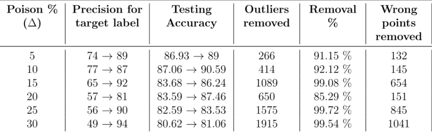
ENRON The ENRON email dataset [51] is a spam email dataset with 4137 training points and 1035 testing points. All data points have 5116 dimensions and are labelled as 1 if it’s spam and 0 otherwise. Furthermore, this dataset has class imbalance with 70% ham emails and 30% spam emails. We simulate label flip attacks as well as adversarially additive attacks for this dataset. For our experiment, we flip labels from Class 0 to Class 1 by varying ∆ from0−30% with an increment of 5%. We train on this dataset using a logistic regression model. As an extension of our study, we study some adversarial attacks on this dataset. We move the experiment to AppendixAas adversarial attacks are slightly out of context for this thesis.

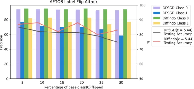
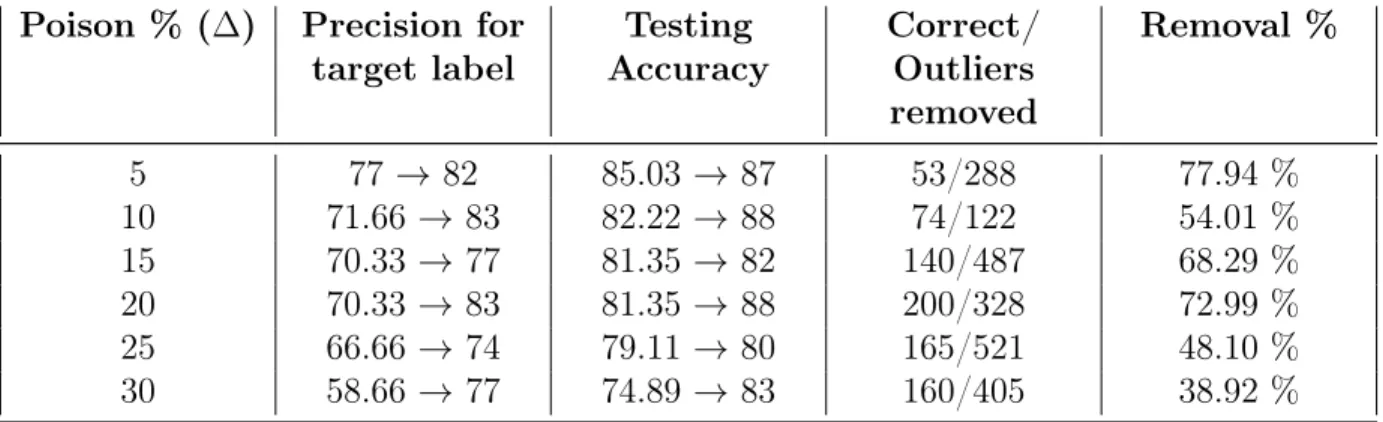
APTOS The APTOS blindness dataset is a large set of 13000 retina images taken using fundus photography under a variety of imaging conditions [32]. These retina images are used to detect diabetic symptoms in a patient using diabetic retinopathy (DR). Each retina image is of different dimensions and belongs to one of 5 classes - 0 - No DR, 1 - Mild, 2 - Moderate. 3 - Severe, 4 - Proliferative DR. For our experiment purpose, we only take a curated subset of this dataset with 3600 points of 224x224 dimensions [33]. We also re-scale each image down to 50% of its original size to 112x112 for ease of computation. Due to high class imbalance in the dataset, we further combine classes 1, 2, 3 and 4 into one class, making it a binary classification task. Similar to ENRON, we create a noisy version of this dataset by flipping class 0 to class 1 by varying ∆ from 0−30% with an increment of5% and train using a logistic regression model.

In Table 6.1, we provide a detailed description of all the different input datasets.

Metrics

Two metrics are used to measure the defence against label flips. First, we report the precision of the target class or how well the model is able to learn the target class. The second metric measures the accuracy of the model on the full testing set — the fraction of the testing examples that are reported correctly. We run each algorithm three times and report the average precision score or testing accuracy. Mathematically, testing accuracy (T A) and Precision (Pa) for class a can be written as follows:

T A= CorrectlyP redicted

T otalP oints Pa=

T rueP ositivesa

T rueP ositivesa+F alseP ositivesa

In the above equation,T rueP ositivesaandF alseP ositivesais defined as the outcomes

where the model correctly predicts class aand model incorrectly predicts some other class instead of a respectively.

(39)

Implementation

All experiments are done on a computer with specifications of 8GB Geforce GTX 1080 GPU, core i7 3.4 GHz processor and 62GB RAM. The source code for our experiments is written in Python using PyTorch, and implementation of DPSGD is used from the Pyvacy [81] library. We carry out experiments using 3 different models. The experiments on APTOS and ENRON are done on a simple logistic regression model. MNIST experiments are done using a 1 hidden layer fully connected Multilayer Perceptron (MLP) with Rectified Linear Unit (ReLU) activation and a CNN model with 2 convolutional layers and a fully connected layer at the end using cross entropy loss. We repeat all the experiments for 3 iterations and report the average.

Dataset Noise Dataset

Size

Classes Model Support in Training Set MNIST i) Targeted Flip from 1 to 7; ii) Weak composite Tweak; iii) Strong composite Tstrong 60000, 10000 10 i) MLP ii) CNN Class 0 - 5923 Class 1 - 6742 Class 2 - 5958 Class 3 - 6131 Class 4 - 5842 Class 5 - 5421 Class 6 - 5918 Class 7 - 6265 Class 8 - 5851 Class 9 - 5949 ENRON Targeted Flip

from 0 to 1

4137, 1035 2 Logistic

Regression

Class 0 - 2928 Class 1 - 1209 APTOS Targeted Flip

from 0 to 1

1857,1805 5 Logistic

Regression

Class 0 - 1372 Class 1 - 1374 Table 6.1: List of datasets

Baseline

For our experiments, we compare_Diffindo against three baselines. Our first baseline is DPSGD [72, 5, 1]. We run DPSGD on the training data with noisy labels for the same privacy budget. IfDiffindodoes not plan to remove any points (Lines 1-10 of Algorithm2

(40)

is compensated by running DPSGD for more number of epochs. One may choose to use the extra privacy budget to decrease the value ofσ, but that might not be sufficient enough for significant improvement compared with extra epochs of training or running_Diffindo. Our second baseline is a private unsupervised clustering algorithm, IMSAT [30]. According to a recent survey [52,3], IMSAT is the state of the art unsupervised deep clustering technique. It uses clustering entropy loss and self augmentation to achieve an accuracy of 98.4% on MNIST. We choose this as our DP baseline because one may wish to ignore the labels and learn the dataset using an unsupervised clustering task. We experiment on IMSAT by applying a differentially private counterpart of the optimizer used in IMSAT called Adam [36]. And our final baseline is the non-private vanilla SGD. We run a non-private version of _Diffindo ( = ∞) and compare it against SGD when trained on the same data with noisy labels. For the non-private scenario for_Diffindo, instead of using a filter condition and threshold for removal, we remove a pre-computed top percentile of points. The percentile is calculated approximately by dividing the 2 times the total number of outliers over total removal iterations (Tf). We do this because our experiments for filter

condition show that_Diffindoperforms best when we remove points in every epoch. This is a smart choice for the non-private scenario now that we can use the FILTER function for free.

6.2 End-to-End Evaluation

In the end-to-end evaluation, we compare _Diffindo with the aforementioned baselines across multiple inputs.

6.2.1 Targeted Strong Label Flips

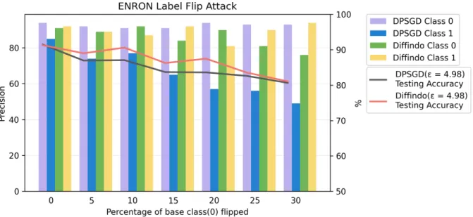
We show the performance of Diffindo on targeted label flip attacks for three different datasets – MNIST, ENRON and APTOS. These datasets are inherently unique. MNIST is a balanced image dataset whereas ENRON is a numerical data and suffers from class imbalance. APTOS is a medical image dataset and is also affected by class imbalanced but has been synthetically balanced by combining multiple output classes. Our experiments show that _Diffindo can improve the testing accuracy and the precision of the targeted label when compared to baseline DPSGD for the same privacy budget for each of the datasets.

(41)

MNIST

In our experiments for MNIST, we run _Diffindo with the following default setting. We set lot size (L) as 250 and run 50 epochs, where each epoch consists of n/L lots. The default values forσ, C and C2 are 1.1, 1and 0.002 respectively. The removal condition in Algorithm 2 is set such that the FILTER function (Algorithm 3) is called after the 10th

epoch in an interval of 3 epochs each. As the removal is done only after 12 epochs of training, we pay for the equivalent cost of an extra24 epochs in the moments accountant analysis. The privacy cost of _Diffindo with this configuration gives as 3.6 with δ as 10−5. The filter multiplierpis set adaptively in every epoch from1.6to2.2times the score of the noisy average gradient by_Diffindo.

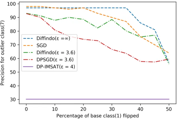
Figure 6.1: _Diffindohas a higher precision than the baseline algorithms (DP-IMSAT and DPSGD).

(42)

and σ, DPSGD can run for a total of 74 epochs, as no privacy budget is required for removing points.

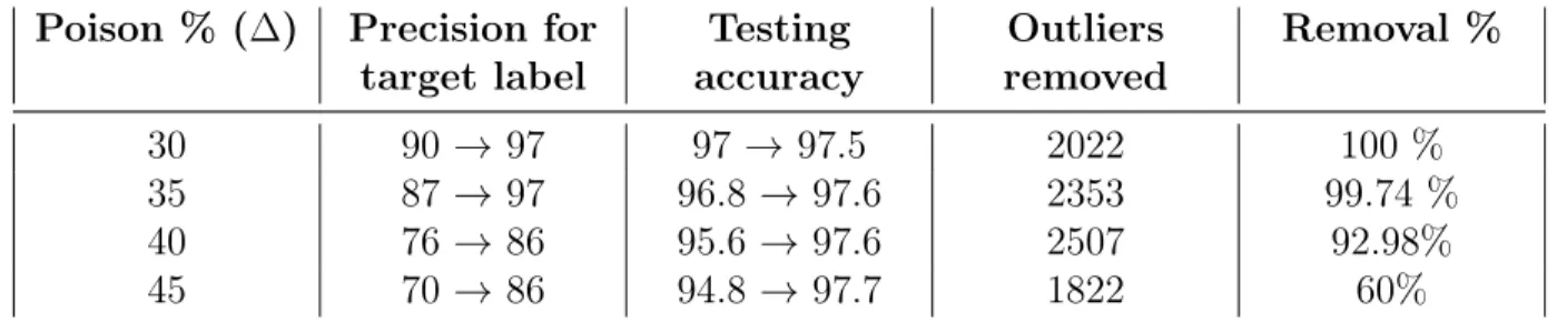
Poison % (∆) Precision for target label Testing accuracy Outliers removed Removal % 30 90→ 97 97→ 97.5 2022 100 % 35 87→ 97 96.8 → 97.6 2353 99.74 % 40 76→ 86 95.6 → 97.6 2507 92.98% 45 70→ 86 94.8 → 97.7 1822 60%

Table 6.2: Results on improvement of accuracy for _Diffindo (= ∞) compare to SGD on MNIST

Poison % (∆) Precision for target label Testing accuracy Outliers removed Removal % 30 66.6 → 88.55 87.7 →92 4220 86.59 % 35 63.7 → 80.2 86.5 → 90.4 4484 86 % 40 57.8 → 75.7 89 →89.74 4647 71.58% 45 57.4 → 77 86.5 → 89.7 4805 59%

Table 6.3: Results on improvement of accuracy for _Diffindo ( = 3.6) compared to DPSGD ( = 3.6) on MNIST

First, we show that our proposed algorithm _Diffindo improves the precision of the target class with respect to the baseline algorithms, DPSGD and DP-IMSAT. As shown in Figure6.1, given the same privacy budget = 3.6, δ= 10−5, _Diffindo (the green dot-dashed line) has a5%to20%higher precision than DPSGD algorithm (the red dot-dashed line), when the fraction of 1s flipped to 7s,∆(T17 element of the noise transition matrix), is between 10% and 40%. When ∆ = 0, there are no noisy labels; both algorithms can achieve similar accuracy given a sufficient amount of iterations. However, when∆ = 50%, both algorithms have relatively poor precision for class 7, as the images for class 1 are no longer outliers to class 7 in the training data. However,_Diffindoand DPSGD have much better precision compared to DP-IMSAT, a private unsupervised learning algorithm. This baseline is delicate to noise and has poor accuracy at any reasonable value of(e.g. = 4.0 in Figure 6.1). The plot for DP-IMSAT is horizontal as it is independent of the labels.

We detail the comparison results between non-private_Diffindoand SGD in Table6.2

Differentially Private Learning with Noisy Labels