A Model of Money and Credit, with
Application to the Credit Card Debt Puzzle
∗
Irina A. Telyukova
University of Pennsylvania
Randall Wright
University of Pennsylvania
May 9, 2006
AbstractMany individuals simultaneously have significant credit card debt and money in the bank. Thecredit card debt puzzleis, given high interest rates on credit cards and low rates on bank accounts, why not pay down the debt? While economists have recently gone to elaborate lengths to explain this observation, we argue that it is nothing more than the venerablerate of return dominance puzzle from monetary economics. We therefore analyze the issue by extending standard monetary theory to incorporate consumer debt. This seems interesting in its own right, since developing models where money and credit coexist is a long-standing challenge, and it helps put into context recent discussions of consumer debt.
∗We thank Neil Wallace, Ed Nosal, and participants in seminars at Penn and the Federal Reserve Banks of Cleveland and New York for feedback. We thank the National Science Foundation and the Jacob K. Javitz Graduate Fellowship Fund for research support. The usual disclaimer applies.
1
Introduction
A large number of households simultaneously have significant credit card debt and a significant amount of money in their checking and savings accounts. Although there are many ways to measure this, a simple summary statistic is that 27% of U.S. households in 2001 had credit card debt in excess of $500 and over $500 in the bank; and the median such household revolved around $3,800 of credit card debt and had $3,000 in the bank (see Telyukova 2005). The so-called
credit card debt puzzle is this: given 14% interest rates on credit cards, and 1 or 2% on bank accounts, why not pay down the debt? “Such behavior is puzzling, apparently inconsistent with no-arbitrage and thus inconsistent with any conventional model.” (Gross and Souleles 2001).
Economists have gone to elaborate lengths to explain this type of phenomena. For example, some people assume that consumers cannot control themselves (Laibson et al. 2000); others assume they cannot control their spouses (Bertaut and Haliassos 2002; Haliassos and Reiter 2003); and still others hypothesize that such households are typically on the verge of bankruptcy (Lehnert and Maki, 2001). While these ideas are interesting, and may contain elements of truth, we think it is useful to point out that the credit card debt puzzle is actually not a new observation. Rather, it is “simply” another ramification of the venerable rate of return dominance puzzle
from monetary economics, and hence, insights may be gained by using models and ideas from monetary theory. In particular, the relevant notion is liquidity.1
Our hypothesis is the following. Households need money — generally, relatively liquid assets — for contingencies where it is difficult or costly to use credit. It is important to note that there are many big-ticket items for which this is the case, over and above the usual examples like taxis and cigarettes. For instance, usually rent or mortgage payments cannot be made by credit card. Also, many less perfectly anticipated events such as household repairs (plumbing, heating, air conditioning, etc.) often require cash, for whatever reason, and getting caught short can be
1
The idea that agents may hold assets with low rates of return because they are relatively liquid — i.e. because they have potential advantages as a medium of exchange — underlies much of modern monetary theory going back to Kiyotaki and Wright (1989). And, as we discuss below, it goes back much further in the less formal literature.
very costly.2 Even if agents are revolving credit card debt, they need to have some cash easily accessible to meet these contingencies. The point may be obvious — but this does not mean that it would not be interesting to analyze it in detail.
The rate of return dominance question and the idea that some notion of liquidity ought to be part of the solution goes back a long time. Hicks (1935) is well known for challenging monetary economists to “look frictions in the face” when framing “the central issue in the pure theory of money” as the need for an explanation of the fact that people hold money when rates of interest are positive. One perhaps better known version of the challenge is to explain “the decision to hold assets in the form of barren money, rather than of interest- or profit-yielding securities.” But the same issue arises in reverse: “So long as interest rates are positive, the decision to hold money rather than lend it, oruse it to pay offold debts, is apparently an unprofitable one” (Hick 1935, p.5, emphasis added).
We believe there is something to be gained by analyzing the credit card debt puzzle in the context of monetary economics, and bringing to bear some of the ideas from modern theory. However, to our knowledge — or maybe, in our opinion — there does not exist an appropriate off-the-shelf model of money and credit that can be used to address the issue. So we build one. While this isnot meant to constitute the last word on rate of return dominance, because we do need some strong assumptions, we think we have a logically consistent economic environment that is useful for this purpose. While our framework builds on some recent results, we also extend existing monetary theory along several dimensions. This is interesting in its own right, since clearly getting coexistence of consumer credit and money in a logically consistent theory is not easy. And from a substantive point of view, it allows us to interpret the coexistence of credit card debt and money in the bank in a very different light vis a vis the literature.3
2According to the U.S. Statistical Abstract, 77% of consumer transactions in 2001 used liquid assets (defined
to include cash, bank deposits, and closely related instruments). According to the Consumer Expenditure Survey, the median household described above (with $3,800 of credit card debt and $3,000 in the bank) spent $1,993 per month on goods purchased with liquid assets (Telyukova 2005).
3This paper is abouttheory; whether the approach is able to accountquantitatively for the salient aspects of
2
The Basic Model
We build on Lagos and Wright (2005), hereafter LW. That model gives agents periodic access to centralized markets, in addition to the decentralized markets where due to frictions money is essential for trade. Having some centralized markets is interesting for its own sake, and also makes the analysis much more tractable than what onefinds in much of the literature on the microfoundations of money.4 However, existing versions of the model have nothing that resembles consumer debt, and as we explain below, it is not easy to get consumer debt into the framework without extending it in just the right way. Here we describe the basic physical environment, for now focusing on a special case; later, we generalize.
A [0,1] continuum of agents live forever in discrete time. There is one nonstorable con-sumption good at each date that agents may (stochastically) be able to produce using labor. There is also money in this economy, a perfectly divisible and storable object that is intrinsically worthless, but potentially could have use as a medium of exchange. The money supply isfixed for now at M, but later we allow it to vary over time. Although we use the word money, we do not necessarily mean cash literally. It is not hard to recast the model with agents depositing cash into bank accounts and paying for goods using checks or debit cards, as in He, Huang and Wright (2005). We discuss this further below. It is relevant because what we have in mind is not moneyper se, but relatively liquid assets more generally.
In LW, each period is divided into two subperiods. In one, there is a centralized Walrasian market, and in the other, there is a decentralized market where agents meet according to a random bilateral-matching process. With the additional assumption that agents are anonymous in the decentralized market, a medium of exchange becomes essential.5 After each meeting of this market agents go to the centralized market, where they engage in various activities that include
4
See Molico (1997), Green and Zhou (1998), Camera and Corbae (1999), Zhou (1999) or Zhu (2003) for models where all trade is decentralized, and the analysis is much more difficult. Earlier models, like Shi (1995) or Trejos and Wright (1995), were also tractable, but only because money was assumed to be indivisible and agents were allowed to hold at most1unit.
5
working and rebalancing their money holdings. If utility is linear in hours worked, all agents take the same amount of money out of the centralized market, which is what keeps the analysis relatively simple; without these assumptions, there is generally an endogenous distribution of money across traders in the decentralized market that one has to track as a state variable.
As we said above, there is no role for credit in LW, and it is important to understand why it is not easy to create such a role. Credit is not possible in the decentralized market because of the assumption that agents are anonymous, which we cannot relax since this is what makes money essential. And credit is not necessary in the centralized market because of the assumption that all agents can work and have utility that is linear in hours, which we do not want to relax since this is what keeps the analysis tractable. How to proceed? Our idea is to introduce another subperiod (we generalize later to many subperiods) with a market where agents may want to consume but cannot produce, which makes credit useful, and where we do not assume anonymity, which makes credit feasible. We determine whether agents use cash or credit in this market endogenously, while maintaining an essential role for money plus analytic tractability due to the other two markets.6
All agents want to consume in subperiod (market) 1, and u1(x1) is their common utility
function. A random subset want to consume in s = 2,3, and conditional on this, us(xs) is their utility function. Assumeus(xs) is strictly increasing and concave. All agents are able to produce in s= 1, and the disutility of working h1 hours is c1(h1) =h1. A random subset are
able to produce ins= 2,3, and conditional on this, the disutility of working is an increasing and convex functioncs(hs).When they can produce, agents transform labor one-for-one into goods,
xs =hs.7 For simplicity, at anys= 2,3a random set of agents chosen in an i.i.d. manner want to consume but cannot produce and vice-versa; no one can do both, but this would be easy to
6Berentsen, Camera and Waller (2005a) also add a third subperiod to LW, but it is another round of
decen-tralized exchange and so there is no possibility of credit. Berentsen et al. (2005b) and Chiu and Meh (2006) introduce a third subperiod with a centralized market in order to discuss banking, as in He et al. (2005); the focus here is on an entirely different set of issues, however.
7
One can assume there is a real wage w that is constant and can be normalized to 1 because there are competitivefirms with linear technologies; it is easy to extend this and introducefirms with general technlologies to determinewendogenously.
relax. Letx∗s denote the solution to u0s(x∗s) =c0s(x∗s). Let βs be the discount factor between s
and the next subperiod, withβ1β2β3<1.
An individual’s state is (mst, bst), denoting money and debt in subperiod s of period t, but we drop the t when there is no risk of confusion; e.g. we write mst = ms, ms,t+1 = ms,+1,
etc. Let Ws(ms, bs) be the value function. At s = 1,2, the market value of money is φs, so
ps = 1/φs is the nominal price level; there there is no φ3 since there is no centralized market
at s = 3, although prices will implicitly be defined by trades. Similarly, the real interest rate in the centralized markets at s= 1,2 is rs, but there is no r3. Our convention for notation is
as follows: if you bring debt bs into subperiod s= 1,2 you owe (1 +rs)bs. The plan now is to consider each subperiod (market) in turn. After this, we put the pieces together and describe equilibrium.
2.1
Market 1
At s= 1, there is a centralized market where agents solve8
W1(m1, b1) = max
x1,h1,m2,b2{u1(x1)−h1+β1W2(m2, b2)} s.t. x1 = h1+φ1(m1−m2)−(1 +r1)b1+b2.
Substituting h1 from the budget constraint into the objective function, we have
W1(m1, b1) = max
x1,m2,b2{u1(x1)−[x1+φ1(m2−m1) + (1 +r1)b1−b2] +W2(m2, b2)}. (1) The first-order conditions are
1 = u01(x1) (2)
φ1 = β1W2m(m2, b2) (3)
−1 = β1W2b(m2, b2). (4)
8To rule out Ponzi schemes, one normally imposes a credit limitb
j≤B¯, either explicitly or implicitly. We do
not need this here because we can explicitly impose that agents pay offpast debts ats= 1each period without loss in generality (due to quasi-linear utility). Also, we always assume an interior solution for h; see LW for conditions to guarantee this is valid in these types of models.
Notice (2) implies x1 =x∗1 for all agents, while (3)-(4) imply (m2, b2) is independent of x1
and (m1, b1) — a feature of quasi-linearity and a generalization of results in LW. As long as W2
is strictly concave, there is a unique solution for (m1, b1). It is simple to check that the same
conditions that guarantee strict concavity in m used by LW also apply here, and so m2 = M
for all agents. However, we will see that W2 is actually linear in b2, which means we cannot
pin down b2 for any individual. This is no surprise with a competitive market and quasi-linear
utility: in equilibrium, agents are indifferent between the allocation they have and an alternative where they work a little more now, save the proceeds, and work a little less later.
Although this is true for any individual, it cannot be true in the aggregate, since the average labor input ¯h1 must equal total output x∗1. Given this, one can resolve the indeterminacy for
individuals in two ways. First, one can focus on symmetric equilibria where all agents choose the same solution when they have the same set of solutions to a maximization problem, which is innocuous since other equilibria are payoff equivalent and observationally equivalent at the aggregate level; this pins down b2 = ¯b2 for all agents. Alternatively, we could impose an
ar-bitrarily small but positive transaction cost on borrowing in subperiod 1, which would break agents’ indifference and refine away all but the symmetric equilibria. In what follows we take the former route, and simply focus on symmetric equilibria.
Aggregating budget equations across agents, we have
¯
x1= ¯h1+φ1( ¯m1−m¯2)−(1 +r1)¯b1+ ¯b2. (5)
In equilibrium, h¯1 = ¯x1 = x∗1, m¯1 = ¯m2 = M, and¯b1 = 0 (average debt must be 0). Hence
(5) implies b2 = ¯b2 = 0 for all agents.9 We close the analysis of market 1 with the envelope
conditions
W1m(m1, b1) = φ1 (6)
W1b(m1, b1) = −(1 +r1), (7)
which imply thatW1 is linear in(m1, b1), another generalization of LW. 9
2.2
Market 2
At s= 2, a measure π of agents want to consume but cannot produce, while a measure π can produce but do not want to consume. In equilibrium, xC2 =hP2, where xC2 is the consumption of consumers and hP2 the production of producers. The expected value of entering market 2 is therefore
W2(m2, b2) =πW2C(m2, b2) +πW2P(m2, b2) + (1−2π)W2N(m2, b2), (8)
where W2C, W2P and W2N are the value functions for a consumer, a producer and a nontrader. We study their problems one at a time, which is slightly tedious, but useful.
For a nontrader,
W2N(m2, b2) = max
m3,b3 β2W3(m3, b3)
s.t. 0 = φ2(m2−m3)−(1 +r2)b2+b3.
Note that although nontraders neither consume nor produce, they can adjust their portfolios.10 The solution(mN3 , bN3 ) satisfies
W3m(mN3 , bN3 ) =−φ2W3b(mN3 , bN3 ), (9)
plus the budget equation. The envelope conditions are
W2Nm(m2, b2) = β2W3m(mN3 , bN3 ) (10) W2Nb(m2, b2) = β2(1 +r2)W3b(mN3 , bN3 ). (11) For a consumer, W2C(m2, b2) = max x2,m3,b3{u2(x2) +β2W3(m3, b3)} s.t. x2 = φ2(m2−m3)−(1 +r2)b2+b3.
1 0It might therefore appear that calling them nontraders is inaccurate, but we will see that in equilibrium they
The solution(xC2, mC3, bC3) satisfies
φ2u02(xC2) = β2W3m(mC3, bC3) (12)
−u02(xC2) = β2W3b(mC3, bC3) (13)
plus the budget equation. Using these, the envelope conditions are
W2Cm(m2, b2) = φ2u02(xC2) =β2W3m(mC3, bC3) (14) W2Cb(m2, b2) = −(1 +r2)u02(x2C) = (1 +r2)β2W3b(mC3, bC3). (15) For a producer, W2P(m2, b2) = max h2,m3,b3{−c2(h2) +β2W3(m3, b3)} s.t.0 = h2+φ2(m2−m3)−(1 +r2)b2+b3.
The solution(hP2, mP3, bP3) satisfies
φ2c02(hP2) = β2W3m(mP3, bP3) (16)
−c02(hP2) = β2W3b(mP3, bP3) (17)
plus the budget equation. The envelope conditions are
W2Pm(m2, b2) = φ2c02(hP2) =β2W3m(mP3, bP3) (18)
W2Pb(m2, b2) = −(1 +r2)c02(hP2) = (1 +r2)β2W3b(mP3, bP3). (19)
We cannot conclude that(m3, b3)is independent of(m2, b2), the way we could conclude that (m2, b2) is independent of(m1, b1)in the previous subperiod. If xC2 depends on(m2, b2) then so
will (mC3, bC3), unlessu2 is linear; and if hP2 depends on (m2, b2) then so will(mP3, bP3), unlessc2
is linear. In any case, we have
W2m(m2, b2) = β2[πW3m(mC3, bC3) +πW3m(mP3, bP3) + (1−2π)W3m(mN3 , bN3 )] (20)
2.3
Market 3
In market 3 trade occurs via anonymous bilateral meetings and bargaining.11 Because of anonymity, you cannot use credit: I will not take your IOU because I understand you could renege, without fear of punishment, given that I do not know who you are. However, one may ask why some institution that is not anonymous cannot issue interest-bearing claims to goods next period that might circulate in market 3. The simplest answer is to assume such claims can be counterfeited. Thus, the government here has a monopoly on the production of non-counterfeitable notes, and chooses to issue only non-interest-bearing money. These assumptions are clearly strong. As suggested above, we do not presume to provide a definitive solution to the rate of return dominance problem; we do think we have a logically consistent environment in which there is a role for money plus credit.12
There is one more issue to address. As we said above, there is a version of the model where agents deposit money in banks and pay with checks or debit cards in decentralized markets, along the lines of He et al. (2005). Checks work even though consumers are anonymous, because they are claims on the bank and not on the consumer personally (think of travellers’ checks as the purest example). In such a model, interest paid on checking accounts is determined endogenously, but it will not equal the market interest rate on consumer credit, as it would in a frictionless market, as long as we adopt one of several assumptions. We can simply assume government prohibition of interest on checking, as was the case for much of U.S. history. Or we can assume the bank has some operating costs. Or we can assume that banks need to hold reserves, either to meet legal requirements or to facilitate settlement.
For example, suppose we have 100% reserve requirements (so-called narrow banking). Then banks earn no revenue from and hence pay no interest on deposits. Indeed, if there are operating costs, they pay negative interest — i.e. they charge a fee for checking privileges. In He et al.
1 1Bargaining is not a crucial part of the specification — versions of related models exist with price taking and
price posting (as in Rocheteau and Wright 2005), and with auctions (once one allows some multilateral meetings, as in Kircher and Galenianos 2006 or Julien, Kennes and King 2006).
1 2
(2005), agents may be willing to deposit money in banks even at negative interest rates for safety reasons (again think of travellers’ checks). As long as banks keep some reserves for whatever reason and/or have some operating costs, the equilibrium interest rate on checking accounts is below the market interest rate. The point is that liquidity comes at a cost. The pure monetary model without banks captures this in an economical way, but it ought to be clear that the underlying ideas apply more generally.
Consider a meeting where one agent wants to consume and the other can produce. Call the former agent thebuyer and the latter theseller. They bargain over the amount of consumption for the buyer x3 and labor by the seller h3, and also a dollar payment dfrom to the former to
the latter. Since feasibility implies x3 =h3, we denote their common value byq. If (m3, b3) is
the state of a buyer and( ˜m3,˜b3) the state of a seller, the outcome satisfies the generalized Nash
bargaining solution,
(q, d)∈arg max S(m3, b3)θS˜( ˜m3,˜b3)1−θ s.t. d≤m3, (22)
whereθ is the bargaining power of the buyer, and the surpluses are given by
S(m3, b3) = u3(q) +β3W1,+1(m3−d, b3)−β3W1,+1(m3, b3) ˜
S( ˜m3,˜b3) = −c3(q) +β3W1,+1( ˜m3+d,˜b3)−β3W1,+1( ˜m3,˜b3).
Using (6) and (7), these simplify to
S(m3, b3) = u3(q)−β3φ1,+1d ˜
S( ˜m3,˜b3) = −c3(q) +β3φ1,+1d.
The constraintd≤m3 in (22) simply says a buyer cannot transfer more money than he has.
Given all this, we have the following generalization of LW (proof is in the Appendix).
Lemma 1. ∀(m3, b3) and ( ˜m3,˜b3), the solution to the bargaining problem is
q= ½ g−1(β3m3φ1,+1) if m3 < m∗3 q∗ if m3 ≥m∗3 and d= ½ m3 if m3< m∗3 m∗3 if m3≥m∗3 (23)
where q∗ solves u03(q∗) =c03(q∗), the functiong(·) is given by
g(q) = θu03(q)c3(q) + (1−θ)u3(q)c03(q)
θu03(q) + (1−θ)c03(q) , (24)
and m∗3 =g(q∗)/β3φ1,+1.
Clearly, the bargaining solution (q, d)depends on the buyer’s money holdingsm3, but on no
other element of (m3, b3) or ( ˜m3,˜b3); hence we write q = q(m3) and d= d(m3) from now on.
Of course,q and datt also depend on φ1 att+ 1, but this is left implicit in the notation. We show in the Appendix that, exactly as in LW,m3< m∗3 in any equilibrium. Hence, from Lemma
1, buyers always spend all their money in market 3, and receive q =g−1(β3m3φ1,+1). Notice
∂q/∂m3=β3φ1,+1/g0(q)>0. It will be useful to define
e(q) = u 0 3(q)
g0(q), (25)
and to assume e0(q) <0. Sufficient conditions on preferences that guarantee e0(q) <0 can be found in LW; a simple condition that works for any preferences is θ ≈ 1, since θ = 1 implies
g(q) =c(q).
Let σ denote the probability of a meeting between a buyer and a seller in market 3. Then
W3(m3, b3) =σ{u3[q(m3)]+β3W1[m3−d(m3), b3]}
+σE{−c3[q( ˜m3)]+β3W1[m3+d( ˜m3), b3]}+ (1−2σ)β3W1[m3, b3], (26)
where Eis the expectation of m˜3 (the money holdings of a random agent one meets, which we
will later show to be degenerate at m˜3 =M). Differentiating (26) and using (6) and (7),
W3m(m3, b3) = β3φ1,+1{σe[q(m3)] + 1−σ} (27)
W3b(m3, b3) = −β3(1 +r1,+1). (28)
As described by (27), the marginal value of money in market 3 is a weighted average of the values of spending it and of carrying it forward to next period, while (28) gives the marginal value of debt as the value of simply rolling it over.
2.4
Equilibrium
Our definition of equilibrium is relatively standard, except that there is no market-clearing condition for market 3: since trade is bilateral in this market, it clears automatically. To reduce notation, we describe every agent’s problem ats= 1,2in terms of choosing(xs, hs, ms+1, bs+1), which are implicitly functions of the state, where it is understood that for producers xP2 = 0, for consumershC2 = 0, and for nontraders xN2 =hN2 = 0.13
Definition 1. An equilibrium is a set of (possibly time-dependent) value functions {Ws},
s = 1,2,3, decision rules {xs, hs, ms+1, bs+1}, s = 1,2, bargaining outcomes {q, d}, and prices {rs, φs}, s= 1,2, such that:
1. Optimization: In every period, for every agent, {Ws}, s= 1,2,3, solve the Bellman
equa-tions (1), (8) and (26); {xs, hs, ms+1, bs+1}, s = 1,2, solve the relevant maximization
problems; and {q, d} solve the bargaining problem. 2. Market clearing: In every period,
¯
xs= ¯hs, m¯s+1=M,¯bs+1= 0, s= 1,2
where for any variable y, y¯=Ryidi denotes the aggregate.
Definition 2. A steady state equilibrium is an equilibrium where the endogenous variables are
constant across time periods (although not generally across subperiods within a period).
We are mainly interested in equilibria where money is valued, which means that it is valued in all subperiods in every period.
Definition 3. A monetary equilibrium is an equilibrium where, in every period,φs>0,s= 1,2,
and q >0.
1 3We do not include the distribution of the state variable in the definition of equilibrium, but it is implicit:
given an initial distributionF1(m, b) at the start of subperiod1, the decision rules generateF2(m, b); then the decision rules ats= 2generateF3(m, b); and the bargaining outcome ats= 3generatesF1,+1(m, b). Also, as we said above, we only consider equilibria where we have an interior solution forh.
We now characterize steady-state equilibria (the steady state requirement is relaxed below). First, recall that in equilibrium we impose that in market 1, if two agents have multiple solutions for b2 they choose the same one. As we discussed above, due to quasi-linear utility, any other
equilibria are payoff equivalent for individuals, and observationally equivalent at the aggregate level. Further, in any of the other equilibria, prices and consumption are exactly the same as stated in the following theorem.
Theorem 1. In any steady state monetary equilibrium:
1. At s= 1, all agents choose x1 =x∗1, m2=M, b2 = 0, and
h1=h1(m1, b1) =x∗1−φ1(m1−M) + (1 +r1)b1,
which implies h¯1 =x∗1.
2. At s= 2,
consumers choose x2 =x∗2, m3=M and b3 =x∗2;
producers chooseh2=x∗2, m3 =M and b3=−x∗2;
nontraders choose m3 =M and b3 = 0.
3. At s= 3, in every trade d=M andq solves
1 + ρ
σ =e(q), (29)
where e(q) is given by (25) and ρis defined by 1
1 +ρ =β1β2β3.
4. Prices are given by:
r1 = u02(x∗2)−β2β3 β2β3 , r2 = ρ−r1 1 +r1 , φ1 = g(q) β3M, and φ2 = φ1[σe(q) + 1−σ] 1 +r1 .
Proof: To begin, insert the envelope condition forW3b from (28) into (13) and (17) to get
u02(xC2) = β2β3(1 +r1,+1) (30)
This impliesu02(xC2) =c02(h2P), and hencexC2 =hP2 =x∗2. Similarly, insert the envelope condition forW3m from (27) in to the first order conditions (12) and (16) to get
φ2u02(xC2) = β2β3φ1,+1©σe£q(mC3)¤+ 1−σª (32)
φ2c02(h2P) = β2β3φ1,+1©σe£q(mP3)¤+ 1−σª. (33)
Givene0(q)<0and q0(m)>0 for allm < m∗3, plus xC2 =hP2 =x2∗, we concludemC3 =mP3. Similarly, inserting (28) and (27) into the first order condition for a nontrader, we get
φ1,+1©σe£q(mN3 )¤+ 1−σª=φ2(1 +r1,+1) (34)
Exactly the same condition results from combining (30) and (32) for a consumer, or (31) and (33) for a producer. Hence, we conclude mN3 =mC3 =mP3 = M. From the budget equations, this means debt is given by
bC3 = x∗2+ (1 +r2)b2
bP3 = −x∗2+ (1 +r2)b2
bN3 = (1 +r2)b2.
This completes the description of market 2. Moving back to market 1, clearly (2) implies
x1 =x∗1. Inserting the envelope conditions forW2 and W3 into (3) and (4), we have
φ1 = β1β2β3φ1,+1{σe[q(M)] + 1−σ} (35)
1 = β1β2β3(1 +r2)(1 +r1,+1), (36)
where we use in thefirst case the result thatW3mdepends onm3but notb3, andm3=M. Notice
(36) is an arbitrage condition betweenr2 andr1,+1: if it does not hold there is no solution to the
agents’ problem ats= 1; and if it does hold then any choice ofb2is consistent with optimization.
Hence we can setb2 = 0. On the other hand, (35) implies
(1 +ρ) φ1
In steady state this implies (29).
The only things left to determine are the prices. We get r1 from (30) with x2 = x∗2, and
then set r2 in terms of r1 to satisfy the arbitrage condition (36). Given q, Lemma 1 tells us
φ1=g(q)/β3M, and (34) gives
φ2 = φ1[σe(q) + 1−σ]
(1 +r1) .
This completes the proof. ¥
The central result of Theorem 1 is that at s = 2, consumers buy on credit (b3 = x∗2) even
though they are holding m3 = M and even though buying on credit entails a cost in terms of
interest. The reason, of course, is that they know they may need the money at s= 3.
We now discuss rates of return. Condition (34) equates the value of a dollar’s worth of cash and a dollar’s worth of credit coming out of market 2. The left side is a weighted average of the marginal gain if the dollar is spent in market 3,u0(q)q0(m3) =β3φ1,+1e(q), and the return if it is not spent but carried forward to the next period, β3φ1,+1. The right side of (34) is the real return (the interest saving) from using the same dollar to pay down debt,β3φ2(1+r1,+1). Notice
the return to money includes aliquidity premium: we show below that e(q)>1in equilibrium, and hence the value to spending a dollar is higher than the value to carrying it to the next period. If one ignores the liquidity premium, and simply considers the return on carrying money across periods, then it looks like — indeed, it is — rate of return dominance.
Theorem 2. (Rate of Return Dominance) In any steady state monetary equilibrium,
φ1,+1 φ2 <1 +r1,+1. Proof: By (34), φ1,+1 φ2 = 1 +r1,+1 1−σ+σe(q).
The result follows if 1−σ+σe(q) > 1, or e(q) > 1. However, by (29), in steady state e(q) =
Two brief comments are in order. First, we can price nominal bonds via the Fisher equation, which is simply a no-arbitrage condition, to get the nominal rate1+i1,+1= (1 +r1,+1)φ2/φ1,+1.
Then Theorem 2 can be equivalently stated as i1,+1 >0. Second, the above results are framed
in terms of rates of return betweens= 2attands= 1att+ 1, because this seems most natural given it is at s= 2that the key decision is made (whether to pay with cash or credit). But we could use returns over the entire period. Froms= 1atttos= 1att+ 1, the gross return on money in steady state is1, while the return on credit (paying down debt) is (1 +r2)(1 +r1,+1).
We readily get(1 +r2)(1 +r1,+1)>1 from (36), given β1β2β3 <1, so obviously rate of return
dominance holds across the entire period.
3
Additional Discussion
As we discuss here, the analysis is easily extended in several ways.14 First, in any equilibrium, and not just in steady state, essentially everything in Theorems 1 and 2 holds, except that (37) does not reduce to (29). However, we can insert g(q) =β3m3φ1,+1 from Lemma 1 to get
(1 +ρ) g(q)
g(q+1) =σe(q+1) + 1−σ. (38)
A monetary equilibrium is a bounded, positive, solution {qt} to (38), along with values for the other objects satisfying the same conditions as above. There exist many equilibrium paths for
{qt} (see Lagos and Wright 2003 for details), but in all equilibria, xs, bs, and rs are exactly as given in Theorem 1. And although φ1 and φ2 vary over time with q, Theorem 2 still holds exactly as stated.
Second, suppose the money supply changes at constant rate γ:M+1 = (1 +γ)M. Then it is
natural to look for equilibria where all real variables, includingq andφM, are constant. Hence,
φ1/φ1,+1= 1 +γ, and (37) becomes
(1 +ρ)(1 +γ) =σe[q(M)] + 1−σ.
1 4We already mentioned that bargaining can be replaced with price taking, posting, or auctions, and the main
Using the Fisher equation, the left side is1 +i, and so we have
1 + i
σ =e(q). (39)
Thus,q is decreasing in i, but this does not affect the real allocation in markets 1 and 2. As is standard, the Friedman rule i= 0 is the lower bound on inflation, and also the optimal policy. At i= 0, the returns on money and credit are the same, and we lose rate of return dominance, but for any i >0 everything is qualitatively the same.
The next point concerns our restriction that claims traded in the centralized market cannot circulate in the decentralized market, other than money, due to the assumption that individuals are anonymous and there is no institution can issue non-counterfeitable securities, other than the monetary authority. This is obviously an extreme assumption, meant to capture in a logically consistent way the idea that money is a relatively liquid asset. Consider the other extreme, where there is some perfectly safe, non-counterfeitable, security other than cash that can be used as a medium of exchange. To be concrete, consider a standard one-period, pure-discount security that sells for price ψ in the centralized market today and pays1 unit of the consumption good in the next centralized market. Assume for now that there is no money and no other consumer credit, only this security, and leta be the amount of it brought into a period.15
To illustrate the idea, it suffices to consider a model with two rather than three subperiods — i.e. the basic LW set up — and it is convenient to add a little heterogeneity. Thus, there are now two types: type 1 are the agents in the benchmark LW model, while type 0 never go to the decentralized market (say, they do not consume or produce that good). Given this, it is convenient to change notation slightly. Let U(x)−h be the common preferences in the centralized market, and letu(q)−c(q)be type 1 preferences in the decentralized market. LetW
and V be the value functions for type 1 in the centralized and decentralized markets, andJ the
1 5
This security cannot be indexed by events that happen to you in the decentralized market, since they are not observable to others, and for simplcity there is no uncertainty in the centralized market, so it is not contingent on anything. We will show there is no role for any other securities. In particular,atakes the place of consumer debtbin the benchmark model, witha=−b, the difference being that nowacan be traded in the decentralized market. As always, we need to rule out Ponzi schemes.
value function for type 0. Also, to reduce notation, assume agents discount across centralized markets attand t+ 1, but not between centralized and decentralized markets.
For type 0,
J(a) = max
x,h,a+1{U(x)−h+βJ+1(a+1)} s.t. x = h+a−ψa+1,
since they do not participate in the decentralized market. For type 1,
W(a) = max
x,h,a+1{U(x)−h+V(a+1)} s.t. x = h+a−ψa+1,
where
V(a) =σ{u[q(a)]+βW[a−d(a)]}+σE{−c[q(˜a)]+βW[a+d(˜a)]}+ (1−2σ)βW(a).
For type 0, thefirst order conditions areU0(x) = 1, which impliesx=x∗, andψ=βW+10 (a+1),
which combined with the envelope condition implies the no-arbitrage conditionψ=β. For type 1, thefirst order conditions are U0(x) = 1and ψ=V0(a+1). Using the envelope condition, plus
V0(a) =σu0(q)q0(a)+(1−σ)β and the bargaining solution βa=g(q), we have
ψ=β[σe(q)+1−σ].
Since we already established ψ=β, we conclude that e(q) = 1, and denote the solution by
q1. As is standard, ifθ= 1thenq1=q∗ and we get thefirst best, while ifθ <1thenq1< q∗and
we do not, but we can do no better by introducing money. Indeed, no one would hold money, since it has a lower return thana, unless we run the Friedman rule, and does no better in terms of liquidity. It is clear that we need to make some assumption to give money an advantage in terms of liquidity if we are to get rate of return dominance.16
1 6See Lagos and Rocheteau (2004), Lagos (2006), and Geromichalos, Licari and Suárez-Lledó (2006) for an
It remains to discuss market clearing. Assume there is a measure 1 of type 0 agents and
N1 of type 1 agents, and that we start at the initial date where everyone has a = 0. From
βa=g(q1), the demand foraby each type 1 agent in thefirst period isg(q1)/β; hence the total demand by type 0 must be −N1g(q1)/β, which is consistent with maximization, given ψ = β.
From the budget constraint, in thefirst period a type0agent sets
h=x+ψa1=x∗−N1g(q1).
At every future t, he must make good on his negative at position, but again sets at+1 = −N1g(q1)/β, and ends up working h = x∗. He therefore has a one-time “seigniorage” gain
(in terms of h) from selling short the asset that others use as a medium of exchange. In any case, it is clear that there is no role for money in this model as specified; and it should also be clear that government has an incentive to rule out the use ofaas a medium of exchange so they can get the “seigniorage” for themselves.
Finally, to close this discussion section, we note the following. Although the baseline three-subperiod model clearly delivers on the main goal — agents carrying debt and money simulta-neously — as long as we make some assumptions that give money a liquidity advantage, it does not have another feature that one mightfind desirable. Namely, our agents do not roll over debt for more than one period; they pay it offeach period in market 1. Of course, they have to pay it offsometime (assuming no Ponzi schemes), and given utility is linear in h ats= 1, this is a good time to do so. But we show in the next section that in a generalized version of the model agents do generally roll over debt.
4
General Model
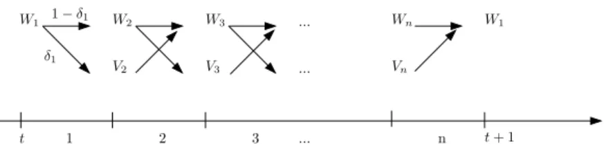
We pursue two generalizations. First, we allow any numbernof subperiods per period (ncould even change over time). Second, there are now centralized and decentralized markets open si-multaneously in every subperiod. Agents visit one market or the other each subperiod according to the following process: an agent in the centralized market atsmoves to the decentralized
mar-... ... W1 W2 W3 Wn W1 V2 V3 Vn t t+ 1 δ1 1−δ1 1 2 3 ... n
Figure 1: Market Structure
ket at s+ 1 with probability δs; and an agent in the decentralized market at s moves to the centralized market at s+ 1with probability1.17 Now agents may want to hold money for every
s, even if this is costly, since they mightfind themselves in need of it at s+ 1.
For convenience, we set δn = 0, so that everyone is in the centralized market at s = 1, and assume all agents can produce with utility linear in hours, as in the benchmark model. For each s∈ {2, ..., n}, the centralized markets are in the spirit of market 2 in the benchmark model, in the sense that credit is available, although we generalize the assumption that some agents cannot produce by now saying that productivity ωs differs randomly in an i.i.d. manner across agents and s (for convenience, ω1 is known and constant across agents). Agents in the
centralized markets ats >1have general utility functionsUs(xs, hs). The decentralized markets are in the spirit of market 3 in the benchmark, in the sense that some agents are buyers, some are sellers, and they meet and bargain bilaterally. Sellers can produce output one-for-one with labor in this market, that is, productivity is not random. Let Ws(ωs, ms, bs) be the centralized and Vs(ms, bs) the decentralized market value function at s. See Figure 1.
At s= 1, everyone is in the centralized market, and solves a problem that is very similar to the centralized market problem in various related models:
W1(ω1, m1, b1) = max
x1,h1,m2,b2{U1(x1)−h1+β1(1−δ1)EW2(ω2, m2, b2) +β1δ1V2(m2, b2)} s.t. x1 = ω1h1+φ1(m1−m2) +b2−(1 +r1)b1
1 7
Thus, agents are never in the decentralized market for two or more periods in a row, which is convenient because it guarantees they are always willing to spend all their money when they get there. This trick is borrowed from Williamson (2005). By the way, the baseline LW model is the special case wheren= 2andδ1= 1.
The first-order conditions are
1/ω1 = U1x(x1) (40)
φ1/ω1 = β1(1−δ1)EW2m(ω2, m2, b2) +β1δ1V2m(m2, b2) (41)
−1/ω1 = β1(1−δ1)EW2b(ω2, m2, b2) +β1δ1V2b(m2, b2). (42)
The envelope conditions are
W1m(ω1, m1, b1) = φ1/ω1 (43)
W1b(ω1, m1, b1) = −(1 +r1) (44)
Again, as in the benchmark model,W1 is linear, everyone chooses the samex1, and(m2, b2) is
independent of(m1, b1).
At s >1, agents in the centralized market solve:18
Ws(ωs, ms, bs) = max
xs,hs,ms+1,bs+1{
Us(xs, hs) +βs(1−δs)EWs+1(ωs+1, ms+1, bs+1) +βsδsVs+1(ms+1, bs+1)}
s.t. xs=ωshs+φs(ms−ms+1) +bs+1−(1 +rs)bs
First-order conditions are
0 = ωsUsx(xs, hs) +Ush(xs, hs) (45)
φsUsx(xs, hs) = βs(1−δs)EWs+1,m(ωs+1, ms+1, bs+1) +βsδsVs+1,m(ms+1, bs+1) (46) −Usx(xs, hs) = βs(1−δs)EWs+1,b(ωs+1, ms+1, bs+1) +βsδsVs+1,b(ms+1, bs+1) (47)
Note (40) is a special case of (45) where U1h(x1, h1) = −1, and (41)-(42) are special cases of
(46)-(47) whereU1x(x1, h1) = 1/ω1. The envelope conditions are
Wsm(ωs, ms, bs) = φsUsx(xs, hs) (48)
Wsb(ωs, ms, bs) = −(1 +rs)Usx(xs, hs). (49)
1 8
In the decentralized market bargaining problem, for simplicity, we setθ= 1in this section. Hence, in equilibrium, ds=ms and qs solves
c(qs) =βsEWs+1[ωs+1,m˜s+ms,(1 +rs)bs]−βsEWs+1[ωs+1,m˜s,(1 +rs)bs], (50)
which can be used to compute q0(ms).19 Also,
Vs(ms, bs) =σE{u(qs) +βsWs+1[ωs+1,0,(1 +rs)bs]}+ (1−σ)βsEWs+1[ωs+1, ms,(1 +rs)bs] and, hence,
Vsm(ms, bs) = σu0(qs)q0(ms) + (1−σ)βsEWs+1,m[ωs+1, ms, bs(1 +rs)] (51)
Vsb(ms, bs) = βs(1 +rs)EWs+1,b[ωs+1, ms, bs(1 +rs)]. (52)
By repeated substitution, the first-order conditions in the centralized market at sforms+1
and bs+1 can be written
φsUsx(xs, hs) = βsβs+1· · ·βnφ1,+1{δs[σe(qs+1) + 1−σ] + (1−δs)δs+1[σe(qs+2) + 1−σ]
+...+ (1−δs)(1−δs+1)· · ·(1−δn−1)} (53)
Usx(xs, hs) = βsβs+1· · ·βn(1 +rs+1)(1 +rs+2)· · ·(1 +r1,+1), (54)
wheree(qs)is defined in (25). By (54)Usx(xs, hs)is constant across agents — i.e. independent of their(ωs, ms, bs) — and hence by (48)-(49)Wsm and Wsb are too. That is,Ws is linear(ms, bs), for all s. Moreover, (50) now implies
qs0(ms) =
βsβs+1· · ·βnφs+1(1 +rs+2)· · ·(1 +r1,+1)
c0(qs) . (55)
Also, (46) now has the following property: the left side is constant and the right side depends onms+1, since this is the only thing that influencesqs+1 which is the only thing that influences
Vs+1,m. In other words, (46) pins down ms+1, independent of (ωs, ms, bs). All agents carry the same amount of money, as in the benchmark model.
1 9
The expectation in this expression is with respect to bothωs+1andm˜s, the money of the seller one meets.
We show below, however, that m˜s = M, exactly as in the benchmark model, andWs is linear in ms, so the
We can summarize what we now know about equilibrium as follows.20 First denote the right side of (54) by ks. Then given ks, (54) for s= 1, ...n, (45) for s = 2, ...n, and (40) constitute
2n−1 equations in2n−1 unknowns, pinning down(¯x1, ...x¯n,¯h2, ...h¯n) (as functions of interest rates). Noticeh1 does not appear in these conditions. We also established thatms+1 =M for
all agents for alls. The centralized market budget equation therefore tells us
bs+1= (1 +rs)bs+ ¯xs−ωsh¯s−φsms+φsM.
This says that agents’ debt ats+ 1 will be equal to their debt ats, all of which is rolled over (principle plus interest), plus consumption expenditure minus labor income, with an adjustment to maintain cash balances at the desired level.21
The key point is that some agents will quite generally carry debt, which is costly in terms of interest, while maintaining a stock of money. When they get to the start of the next period, they pay offtheir debts by adjustingh1,+1. In particular, an agent that draws a lowωswill not only have a low wage, he will additionally have a low hs, since
∂hs
∂ωs
= −ksUsxx
UsxxUshh−Usxh2
>0
by virtue of (45). His consumption may be higher or lower, depending on the cross-derivative of U, since ∂xs ∂ωs = ksUsxh UsxxUshh−Usxh2 .
For example, if U is separable in xs and hs, he will not lower xs. He will often purchase part of xs on credit while maintaining ms+1 =M. When ωs is small andms=M, he will purchase most ofxs on credit while not adjusting his money holdings. In the worst-case scenario, when
ωsis small and ms= 0, he purchases current goods on credit and also takes out a cash advance. We collect some key results from this analysis as follows.
2 0
We do not provide a formal definition of equilibrium here since it is an obvious generalization of the definitions in the benchmark model.
2 1
An individual’smsmay be above (below) his desired level fors+ 1if he just returned from the decentralized
market where he acted as a seller (buyer). In general, ifδs varies withsthen desired real balances will, too; since
Theorem 3. In the model with n subperiods, in any monetary equilibrium,
1. For all s, every agent leaves the centralized market with the samems+1.
2. For all s, Usx(xs, hs) =ks andUsh(xs, hs) =−ksωs where ks is constant across agents in
the centralized market.
3. If two agents have different(ms, bs) and the sameωs, theirhs, xs andms+1 are the same,
so they have differentbs+1; if two agents have the same (ms, bs) and different ωs, theirhs
will differ and they typically have different bs+1.
4. Agents may roll over or run up debts between s = 2 and s = n while maintaining, and
sometimes even increasing, their holdings ofms.
Theorem 4. (Rate of Return Dominance) In any monetary equilibrium, for all s6=n,
φ1,+1
φs <(1 +rs+1)(1 +rs+2)...(1 +rn)(1 +r1,+1) (56)
To say a little more about Theorem 4, a dollar held at smay be spent in the decentralized market in any of the subperiods that follow; or it may not, in which case it is brought into
t+ 1 where it yields ex post return φ1,+1/φs. Alternatively, a dollar at s of consumer credit yields compound interest between then andt+ 1given by the right side of (56). The inequality indicates, as always, that the true value of money is greater than the return from simply carrying it into t+ 1 with probability 1, since it has liquidity value. In particular, from the first-order conditions forms+1 and bs+1 we get
φ1,+1
φs {δs[σe(qs+1) + 1−σ] + (1−δs)δs+1[σe(qs+2) + 1−σ]
+...+ (1−δs)(1−δs+1)...(1−δn−1)}
= (1 +rs+1)(1 +rs+2)...(1 +rn)(1 +r1,+1) (57)
5
Conclusion
In this paper we have tried to re-visit a classic issue: the coexistence of assets with different returns. An example of this issue is the so-called credit card debt puzzle, but more generally, it is known as rate of return dominance. We build on the recent monetary theory literature by allowing the option to sometimes trade using credit. Our model is tractable. It yields strong and interesting outcomes, including the prediction that agents may purchase on credit, even when this has a cost in terms of interest and they have liquid assets at hand. While we think that there is more theoretical work to be done on rate of return dominance, and certainly more quantitative work to be done, we hope this constitutes progress.
References
[1] Berentsen, A., G. Camera and C. Waller. 2005. “Money, Credit and Banking.” Journal of Economic Theory, forthcoming.
[2] Berentsen, A., G. Camera and C. Waller. 2005. “The Distribution of Money Balances and the Non-Neutrality of Money.”International Economic Review, 46(2): 465-487.
[3] Bertaut, C. and M. Haliassos. 2002. “Debt Revolvers for Self Control". University of Cyprus.
[4] Camera, G. and D. Corbae. 1999. “Money and Price Dispersion.” International Economic Review 40(4): 985-1008.
[5] Geromichalos, Athanasios, Juan Licari and José Suárez-Lledó. 2006. “Monetary Policy and Asset Prices.” Mimeo, University of Pennsylvania.
[6] Green, Edward, and Ruilin Zhou. 1998. “A Rudimentary Model of Search with Divisible Money and Prices.”Journal of Economic Theory 81(2): 252-271.
[7] Haliassos, Michael and Reiter, M. 2005. “Credit Card Debt Puzzles". University of Cyprus.
[8] He, Ping, Lixin Huang and Randall Wright. 2005. “Money and Banking in Search Equilib-rium.”International Economic Review, 46(2): 637-670.
[9] Kircher, P. and M. Galenianos. 2006. “Dispersion of Money Holdings and Inflation.” Mimeo, University of Pennsylvania.
[10] Kocherlakota, Narayana. 1998. “Money is Memory.” Journal of Economic Theory 81(2): 232-251.
[11] Lagos, Ricardo. 2006. “Asset Prices and Liquidity in and Exchange Economy.” Federal Reserve Bank of Minneapolis StaffReport 373.
[12] Lagos, Ricardo and Guillaume Rocheteau. 2004. “Money and Capital as Competing Media of Exchange.” Federal Reserve Bank of Minneapolis StaffReport 341.
[13] Lagos, Ricardo and Randall Wright. 2003. “Dynamics, Cycles and Sunspot Equilibria in Genuinely Dynamic, Fundamentally Disaggregative Models of Money.”Journal of Economic Theory 109: 156-71.
[14] Lagos, Ricardo and Randall Wright. 2005. “A Unified Framework for Monetary Theory and Policy Analysis.”Journal of Political Economy, 113: 463-484.
[15] Lehnert, A. and Maki, D. M. 2002. “Consumption, Debt and Portfolio Choice: Testing the Effect of Bankruptcy Law.” Board of Governors of the Federal Reserve.
[16] Molico, Miguel. 1997. “The Distribution of Money and Prices in Search Equilibrium.” In-ternational Economic Review, forthcoming.
[17] Rocheteau, Guillaume and Randall Wright. 2005. “Money in Search Equilibrium, in Com-petitive Equilibrium, and in ComCom-petitive Search Equilibrium.”Econometrica, 73: 175-202.
[18] Shi, Shouyong. 1995. “Money and Prices: A Model of Search and Bargaining.”Journal of Economic Theory 67(2): 467-496.
[19] Telyukova, Irina A. 2005. “Household Need for Liquidity and the Credit Card Debt Puzzle.” Mimeo, University of Pennsylvania.
[20] Trejos, Alberto and Randall Wright. 1995. “Search, Bargaining, Money and Prices.”Journal of Political Economy 103(1): 118-141.
[21] Wallace, Neil. 2001. “Whither Monetary Economics?” International Economic Review
42(4): 847-870.
[22] Williamson, Stephen. 2004. “Search, Limited Participation and Monetary Policy.” Interna-tional Economic Review, forthcoming.
[23] Zhou, Ruilin. 1999. “Individual and Aggregate Real Balances in a Random-Matching Model.”International Economic Review 40(4): 1009-1038.
[24] Zhu, Tao. 2003. “Existence of a Monetary Steady State in a Matching Model: Indivisible Money.”Journal of Economic Theory.
Appendix
In this Appendix we do several things. First we derive the bargaining solution given in Lemma 1. The necessary and sufficient conditions for (22) are
θ£β3φ1,+1d−c3(q) ¤ u03(q) = (1−θ)£u3(q)−β3φ1,+1d ¤ c03(q) (58) θ£β3φ1,+1d−c3(q) ¤ β3φ1,+1 = (1−θ)£u3(q)−β3φ1,+1d ¤ β3φ1,+1 (59) −λ£u3(q)−β3φ1,+1d ¤1−θ£ β3φ1,+1d−c3(q) ¤θ
where λ is the Lagrange multiplier ond≤m3. There are two possible cases: If the constraint
does not bind, then λ= 0, q =q∗ and d=m∗. If the constraint binds then q is given by (58) withd=m3, as claimed.
We now argue that m3 < m∗3. First, as is standard, in any equilibrium φ1,+1 ≤ (1 +ρ)φ1;
this just says the nominal interest rateiis nonnegative. In fact, again as is standard, although we allowi→0, we only consider equilibria wherei >0, so thatφ1,+1 <(1 +ρ)φ1. Now suppose
m3 > m∗3 at some date for some agent. Since the bargaining solution tells us he never spends
more than m∗
3, he could reduce m3 by reducing h1 at t, then increase h1 at t+ 1 so that he
need not change anything else. It is easy to check that this increases utility, som3 > m∗3 cannot
occur in any equilibrium.
Hence m3 ≤m∗3. To show the strict inequality, supposem3 =m∗3 for same agent. Again he
can reduceh1 attand carry less money. If he is a buyer in subperiod 3, he gets a smallerq, but
the continuation value is the same since by the bargaining solution he still spends all his money. If he does not buy then he can increaseh1 att+ 1so that he need not change anything else. It