A Comparison of Distributed Spatial Data Management Systems for Processing Distance Join Queries

A Comparison of Distributed Spatial

Data Management Systems for Processing

Distance Join Queries

Francisco Garc´ıa-Garc´ıa1,?_{, Antonio Corral}1,?_{, Luis Iribarne}1,?_,

George Mavrommatis2_{, and Michael Vassilakopoulos}2,?

1

Dept. of Informatics, University of Almeria, Almeria, Spain. E-mail:{paco.garcia,acorral,liribarn}@ual.es 2

DaSE Lab, Dept. of Electrical and Computer Eng., University of Thessaly, Volos, Greece. E-mail:gmav,mvasilako@uth.gr

Abstract. Due to the ubiquitous use of spatial data applications and the large amounts of spatial data that these applications generate, the processing of large-scale distance joins in distributed systems is beco-ming increasingly popular. Two of the most studied distance join queries are theKClosest Pair Query (KCPQ) and the εDistance Join Query (εDJQ). TheKCPQ finds theKclosest pairs of points from two datasets and theεDJQ finds all the possible pairs of points from two datasets, that are within a distance thresholdεof each other. Distributed cluster-based computing systems can be classified in Hadoop-cluster-based and Spark-based systems. Based on this classification, in this paper, we compare two of the most current and leading distributed spatial data manage-ment systems, namely SpatialHadoop and LocationSpark, by evaluating the performance of existing and newly proposed parallel and distributed distance join query algorithms in different situations with big real-world datasets. As a general conclusion, while SpatialHadoop is more mature and robust system, LocationSpark is the winner with respect to the total execution time.

Keywords:Spatial Data Processing, Distance Joins, SpatialHadoop, LocationSpark.

1

Introduction

Nowadays, the volume of available spatial data (e.g. location, routing, naviga-tion, etc.) is increasing hugely across the world-wide. Recent developments of spatial big data systems have motivated the emergence of novel technologies for processing large-scale spatial data on clusters of computers in a distributed fashion. These Distributed Spatial Data Management Systems (DSDMSs) can be classified in disk-based [9] and in-memory [19] ones. The disk-based DSDMSs are characterized by being Hadoop-based systems and the most representative ones

?

are Hadoop-GIS [1] and SpatialHadoop [6]. The Hadoop-based systems enable to execute spatial queries using predefined high-level spatial operators without having to worry about fault tolerance and computation distribution. On the other hand, the in-memory DSDMSs are characterized as Spark-based systems and the most representative ones are SpatialSpark [15], GeoSpark [17], Simba [14] and LocationSpark [12, 13]. The Spark-based systems allow users to work on distributed in-memory data without worrying about the data distribution mechanism and fault-tolerance.

Distance join queries (DJQs) have received considerable attention from the database community, due to their importance in numerous applications, such as spatial databases and GIS, data mining, multimedia databases, etc. DJQs are costly queries because they combine two datasets taking into account a dis-tance metric. Two of the most representative ones are theK Closest Pair Query (KCPQ) and the ε Distance Join Query (εDJQ). Given two point datasets P

and Q, the KCPQ finds theK closest pairs of points fromP×Qaccording to

a certain distance function (e.g., Manhattan, Euclidean, Chebyshev, etc.). The

εDJQfinds all the possible pairs of points from_P×Q, that are within a distance

thresholdεof each other. Several research works have been devoted to improve the performance of these queries by proposing efficient algorithms in centralized environments [2, 10]. But, with the fast increase in the scale of the big input datasets, processing large data in parallel and distributed fashions is becoming a popular practice. For this reason, a number of parallel algorithms for DJQs in MapReduce [3] and Spark [18] have been designed and implemented [7, 13].

Apache Hadoop1 _{is a reliable, scalable, and efficient cloud computing} fra-mework allowing for distributed processing of large datasets using MapReduce programming model. However, it is a kind of disk-based computing framework, which writes all intermediate data to disk betweenmapandreducetasks. MapRe-duce [3] is a framework for processing and managing large-scale datasets in a distributed cluster. It was introduced with the goal of providing a simple yet po-werful parallel and distributed computing paradigm, providing good scalability and fault tolerance mechanisms. Apache Spark2 is a fast, reliable and distribu-ted in-memory large-scale data processing framework. It takes advantage of the Resilient Distributed Dataset (RDD), which allows transparently storing data in memory and persisting it to disk only if it is needed [18]. Hence, it can reduce a huge number of disk writes and reads to outperform the Hadoop platform. Since Spark maintains the status of assigned resources until a job is completed, it reduces time consumption in resource preparation and collection.

Both Hadoop and Spark have weaknesses related to efficiency when applied to spatial data. A main shortcoming is the lack of any indexing mechanism that would allow selective access to specific regions of spatial data, which would in turn yield more efficient query processing algorithms. A solution to this problem is an extension of Hadoop, called SpatialHadoop [6], which is a framework that supports spatial indexing on top of Hadoop, i.e. it adopts two-level index

struc-1

Available athttps://hadoop.apache.org/ 2

ture (global and local) to organize the stored spatial data. And other possible solution is LocationSpark [12, 13], which is a spatial data processing system built on top of Spark and it employs various spatial indexes for in-memory data.

In the literature, up to now, there are only few comparative studies between Hadoop-based and Spark-based systems. The most representative one is [11], for a general perspective. But, for comparing DSDMSs, we can find [16, 17, 8]. Motivated by this fact, in this paper we compare SpatialHadoop and Locati-onSpark for distance-based join query processing, in particular for KCPQ and

εDJQ, in order to provide criteria for adopting one or the other DSDMS. The contributions of this paper are the following:

– Novel algorithms in LocationSpark (the first ones in the literature) to per-form efficient parallel and distributedKCPQ andεDJQ, on big real-world spatial datasets

– The execution of a set of experiments for comparing the performance of the two DSDMSs (SpatialHadoop and LocationSpark).

– The execution of a set of experiments for examining the efficiency and the scalability of the existing and new DJQ algorithms.

This paper is organized as follows. In Section 2, we review related work on Hadoop-based and Spark-based systems that support spatial operations and pro-vide the motivation for this paper. In Section 3, we present preliminary concepts related to DJQs, SpatialHadoop and LocationSpark. In Section 4, the paral-lel algorithms for processing KCPQ andεDJQ in LocationSpark are proposed. In Section 5, we present representative results of the extensive experimentation that we have performed, using real-world datasets, for comparing these two cloud computing frameworks. Finally, in Section 6, we provide the conclusions arising from our work and discuss related future work directions.

2

Related Work and Motivation

Researchers, developers and practitioners worldwide have started to take advan-tage of the cluster-based systems to support large-scale data processing. There exist several cluster-based systems that support spatial queries over distributed spatial datasets and they can be classified in Hadoop-based and Spark-based sys-tems. The most important contributions in the context of Hadoop-based systems are the following research prototypes:

– Hadoop-GIS[1] extends Hive and adopts Hadoop Streaming framework and integrates several open source software packages for spatial indexing and ge-ometry computation. Hadoop-GIS only supports data up to two dimensions and two query types: rectangle range query and spatial joins.

– SpatialHadoop[6] is an extension of the MapReduce framework [3], based on Hadoop, with native support for spatial 2d data (see section 3.2).

On the other hand, the most remarkable contributions in the context of Spark-based systems are the following prototypes:

– SpatialSpark [15] is a lightweight implementation of several spatial operati-ons on top of the Spark in-memory big data system. It targets at in-memory processing for higher performance. SpatialSpark adopts data partition stra-tegies like fixed grid or kd-tree on data files in HDFS and builds an index to accelerate spatial operations. It supports range queries and spatial joins over geometric objects using conditions likeintersect andwithin.

– GeoSpark [17] extends Spark for processing spatial data. It provides a new abstraction called Spatial Resilient Distributed Datasets (SRDDs) and a few spatial operations. It allows an index (e.g. Quadtree and R-tree) to be the object inside each local RDD partition. For the query processing point of view, GeoSpark supports range query,KNNQ and spatial joins over SRDDs. – Simba (Spatial In-Memory Big data Analytics) [14] offers scalable and effi-cient in-memory spatial query processing and analytics for big spatial data. Simba is based on Spark and runs over a cluster of commodity machines. In particular, Simba extends the Spark SQL engine to support rich spatial queries and analytics through both SQL and the DataFrame API. It intro-duces partitioning techniques (e.g. STR), indexes (global and local) based on R-trees over RDDs in order to work with big spatial data and complex spatial operations (e.g. range query,KNNQ, distance join andKNNJQ). – LocationSpark [12, 13] is an efficient in-memory distributed spatial query

processing system (see section 3.3 for more details).

As we have seen, there are several distributed systems based on Hadoop or Spark for managing spatial data, but there are not many articles comparing them with respect to spatial query processing. The only contributions in this regard are [16, 17, 8]. In [16, 17], SpatialHadoop is compared with SpatialSpark and GeoSpark, respectively, for spatial join query processing. In [8], SpatialHa-doop is compared with GeoSpark with respect to the architectural point of view. Motivated by these observations, and since KCPQ [7] is implemented in Spa-tialHadoop (its adaptation to εDJQ is straightforward), and in LocationSpark neitherKCPQ norεDJQ have been implemented yet, we design and implement both DJQs in LocationSpark. Moreover, we develop a comparative performance study between SpatialHadoop and LocationSpark forKCPQ andεDJQ.

3

Preliminaries and Background

In this section, we first present the basic definitions of the KCPQ andεDJQ, followed by a brief introduction of the preliminary concepts about SpatialHadoop and LocationSpark, the DSDMSs to be compared.

3.1 The K Closest Pairs andε Distance Join Queries

The KCPQ discovers the K pairs of data formed from the elements of two datasets having the K smallest distances between them (i.e. it reports only the top K pairs). The formal definition of the KCPQ for point datasets (the

extension of this definition to other, more complex spatial objects – e.g. line-segments, objects with extents, etc. – is straightforward) is the following: Definition 1. (K Closest Pairs Query, KCPQ)

Let P={p0, p1,· · ·, pn−1} andQ={q0, q1,· · ·, qm−1} be two set of points, and a numberK∈N+. Then, the result of theK Closest Pairs Query is an ordered

collection, KCP Q(P,Q, K), containingK different pairs of points fromP×Q,

ordered by distance, with theK smallest distances between all possible pairs:

KCP Q(P,Q, K) = ((p1, q1),(p2, q2),· · ·,(pK, qK)), (pi, qi)∈P×Q, 1≤i≤K,

such that for any (p, q) ∈ P×Q\KCP Q(P,Q, K) we have dist(p1, q1) ≤

dist(p2, q2) ≤ · · · ≤ dist(pK, qK) ≤ dist(p, q).

Note that if multiple pairs of points have the sameK-th distance value, more than one collection ofK different pairs of points are suitable as a result of the query. Recall thatKCPQ is implemented in SpatialHadoop [7] using plane-sweep algorithms [10], but not in LocationSpark.

On the other hand, theεDJQ reports all the possible pairs of spatial objects from two different spatial objects datasets, P andQ, having a distance smaller

than a distance thresholdεof each other [10]. The formal definition ofεDJQ for point datasets is the following:

Definition 2. (ε Distance Join Query,εDJQ)

Let _P = {p0, p1,· · ·, pn−1} and Q = {q0, q1,· · ·, qm−1} be two set of points, and a distance threshold ε ∈ R≥0. Then, the result of the εDJQ is the set,

εDJ Q(_P,_Q, ε)⊆_P×_Q, containing all the possible different pairs of points from

P×Qthat have a distance of each other smaller than, or equal toε:

εDJ Q(_P,_Q, ε) ={(pi, qj)∈P×Q : dist(pi, qj) ≤ ε}

TheεDJQ can be considered as an extension of the KCPQ, where the dis-tance threshold of the pairs is known beforehand and the processing strategy (e.g. plane-sweep technique) can be the same as in the KCPQ for generating the candidate pairs of the final result. For this reason, its adaptation to Spati-alHadoop from KCPQ is straightforward. Note that εDJQ is not implemented in LocationSpark.

3.2 SpatialHadoop

SpatialHadoop [6] is a full-fledged MapReduce framework with native support for spatial data. It is an efficient disk-based distributed spatial query proces-sing system. Note that MapReduce [3] is a scalable, flexible and fault-tolerant programming framework for distributed large-scale data analysis. A task to be performed using the MapReduce framework has to be specified as two phases: themapphase is specified by amap functiontakes input (typically from Hadoop Distributed File System (HDFS) files), possibly performs some computations on this input, and distributes it to worker nodes; and thereduce phase which pro-cesses these results as specified by a reduce function. Additionally, a combiner

function can be used to run on the output of map phase and perform some filtering or aggregation to reduce the number of keys passed to thereducer.

SpatialHadoop is a comprehensive extension to Hadoop that injects spatial data awareness in each Hadoop layer, namely, the language, storage, MapReduce, and operations layers.MapReduce layer is the query processing layer that runs MapReduce programs, taking into account that SpatialHadoop supports spati-ally indexed input files. TheOperationlayer enables the efficient implementation of spatial operations, considering the combination of the spatial indexing in the storage layer with the new spatial functionality in theMapReduce layer. In ge-neral, a spatial query processing in SpatialHadoop consists of four steps [6, 7] (see Figure 1): (1) Preprocessing, where the data is partitioned according to a specific spatial index, generating a set of partitions or cells. (2) Pruning, when the query is issued, where the master node examines all partitions and prunes by a filter function those ones that are guaranteed not to include any possible result of the spatial query. (3) Local Spatial Query Processing, where a local spatial query processing is performed on each non-pruned partition in parallel on different machines (map tasks). Finally, (4)Global Processing, where the re-sults are collected from all machines in the previous step and the final result of the concerned spatial query is computed. Acombine function can be applied in order to decrease the volume of data that is sent from themap task. Thereduce function can be omitted when the results from themap phase are final.

Fig. 1.Spatial query processing in SpatialHadoop [6, 7].

3.3 LocationSpark

LocationSpark [12, 13] is a library in Spark that provides an API for spatial query processing and optimization based on Spark’s standard dataflow opera-tors. It is an efficient in-memory distributed spatial query processing system. LocationSpark provides several optimizations to enhance Spark for managing spatial data and they are organized by layers: memory management, spatial in-dex, query executor, query scheduler, spatial operators and spatial analytical. In theMemory Management layer for spatial data, LocationSpark dynamically caches frequently accessed data into memory, and stores the less frequently used data into disk. For the Spatial Index layer, LocationSpark builds two levels of

spatial indexes (global and local). To build a global index, LocationSpark sam-ples the underlying data to learn the data distribution in space and provides a grid and a region Quadtree. In addition, each data partition has a local index (e.g., a grid local index, an R-tree, a variant of the Quadtree, or an IR-tree). Finally, LocationSpark adopts a new Spatial Bloom Filter to reduce the com-munication cost when dispatching queries to their overlapping data partitions, termed sFilter, that can speed up query processing by avoiding needless com-munication with data partitions that do not contribute to the query answer. In theQuery Executor layer, LocationSpark evaluates the runtime and memory usage trade-offs for the various alternatives, and then, it chooses and executes the better execution plan on each slave node. LocationSpark has a new layer, termed Query Scheduler, with an automatic skew analyzer and a plan optimi-zer to mitigate query skew. The query scheduler uses a cost model to analyze the skew to be used by the spatial operators, and a plan generation algorithm to construct a load-balanced query execution plan. After plan generation, local computation nodes select the proper algorithms to improve their local perfor-mance based on the available spatial indexes and the registered queries on each node. For theSpatial Operators layer, LocationSpark supports spatial querying and spatial data updates. It provides a rich set of spatial queries including spa-tial range query,KNNQ, spatial-join, andKNNJQ. Moreover, it supports data updates and spatio-textual operations. Finally, for theSpatial Analytical layer, and due to the importance of spatial data analysis, LocationSpark provides spa-tial data analysis functions including spaspa-tial data clustering, spaspa-tial data skyline computation and spatio-textual topic summarization. Since our main objective is to include the DJQs (KCPQ andεDJQ) into LocationSpark, we are interested in theSpatial Operators layer, where we will implement them.

Fig. 2.Spatial query processing for DJQs in LocationSpark, based on [13].

To process spatial queries, LocationSpark builds a distributed spatial index structure for in-memory spatial data. As we can see in Figure 2, for DJQs, given two datasets_Pand_Q,_Pis partitioned intoN partitions based on a spatial index criteria (e.g. N leaves of a R-tree) by the Partitioner leading to the PRDD (Global Index). The sFilter determines whether a point is contained inside a spatial range or not. Next, eachworker has a local data partition _Pi (1 ≤i≤

N) and builds a Local Index (LI). QRDD is generated from _Q by a member function of RDD (Resilient Distributed Dataset) natively supported by Spark,

that forwards such point to the partitions that spatially overlap it. Now, each point of _Q is replicated to the partitions that are identified using the PRDD (Global Index), leading to the Q’RDD. Then a post-processing step (using the Skew Analyzer and the Plan Optimizer) is performed to combine the local results to generate the final output.

4

DJQ Algorithms in SpatialHadoop and LocationSpark

SinceKCPQ is already implemented in SpatialHadoop [7], in this section, we will present how we can adapt KCPQ to εDJQ in SpatialHadoop and how KCPQ andεDJQ can be implemented in LocationSpark.

4.1 KCPQ and εDJQ in SpatialHadoop

In general, theKCPQ algorithm in SpatialHadoop [7] consists of a MapReduce job. Themapfunction aims to find theKCP between each local pair of partitions from_Pand_Qwith a particular plane-sweepKCPQ algorithm [10] and the result is stored in a binary max heap (called LocalKMaxHeap). The reduce function aims to examine the candidate pairs of points from each LocalKMaxHeap and return the final set of the K closest pairs in another binary max heap (called GlobalKMaxHeap). To improve this approach, for reducing the number of pos-sible combinations of pairs of partitions, we need to find in advance an upper bound of the distance value of theK-th closest pair of the joined datasets, cal-led β. This β computation can be carried out by sampling globally from both datasets or by sampling locally for an appropriate pair of partitions and, then executing a plane-sweepKCPQ algorithm over both samples.

The method for the εDJQ in MapReduce, adapting fromKCPQ in Spati-alHadoop [7], adopts themap phase of the join MapReduce methodology. The idea is to have P andQpartitioned by some method (e.g., Grid) into two sets

of cells, with nand mcells of points, respectively. Then, every possible pair of cells is sent as input for the filter function. This function takes as input, com-binations of pairs of cells in which the input set of points are partitioned and a distance thresholdε, and it prunes pairs of cells which have minimum distances larger than ε. By using SpatialHadoop built-in function MinDistance we can calculate the minimum distance between two cells (i.e. this function computes the minimum distance between the two MBRs, Minimum Bounding Rectangles, of the two cells). On the map phase, each mapper reads the points of a pair of filtered cells and performs a plane-sweep εDJQ algorithm [10] (variation of the plane-sweep-basedKCPQ algorithm) between the points inside that pair of cells. The results from all mappers are just combined in the reduce phase and written into HDFS files, storing only the pairs of points with distance up toε. 4.2 KCPQ and εDJQ in LocationSpark

Assuming that _P is the largest dataset to be combined and _Q is the smallest one, and following the ideas presented in [13], we can describe the Execution

Plan for KCPQ in LocationSpark as follows. In Stage 1, the two datasets are partitioned according to a given spatial index schema. In Stage 2, statistic data is added to each partition,S_P andS_Q, and they are combined by pairs, S_PQ. In Stage 3, the partitions from_Pand_Qwith the largest density of points,_Pβ and Qβ, are selected to be combined by using a plane-sweepKCPQ algorithm [10]

to compute an upper bound of the distance value of theK-th closest pair (β). In Stage 4, the combination of all possible pairs of partitions fromPandQ,SPQ, is

filtered according to theβ value (i.e. only the pairs of partitions with minimum distance between the MBRs of the partitions is smaller than or equal to β are selected), giving rise to F S_PQ, and all pairs of filtered partitions are processed by using a plane-sweepKCPQ algorithm. Finally, the results are merged to get the final output.

With the previous Execution Plan and increasing the size of the datasets, the execution time increases considerably due to skew and shuffle problems. To solve it, we modify Stage 4 with the query plan that is used for the algorithms shown in [13], leaving the plan as shown in Figure 3.

Fig. 3.Execution Plan forKCPQ in LocationSpark, based on [13].

Stages 1, 2 and 3 are still used to calculate the β value which will serve to accelerate the local pruning phase on each partition. In Stage 4, using the Query Plan Scheduler,Pis partitioned intoPSandPNSbeing the partitions that

present and do not present skew, respectively. The same partitioning is used to

Q. In Stage 5, a KCPQ algorithm [10] is applied between points of PS and QS

that are in the same partition and likewise for PNS andQNS in Stage 6. These

two stages are executed independently and the results are combined in Stage 7. Finally, it is still necessary to calculate if there is any present candidate for each partition that is on the boundaries of that same partition in the other dataset. To do this, we use β0 which is the maximum distance from the current set of candidates as a radius of a range filter with center in each partition to obtain possible new candidates on those boundaries. The calculation ofKCPQ of each partition with its candidates is executed in Stages 8 and 9 and these results are combined in Stage 10 to obtain the final answer.

TheExecution Plan forεDJQ in LocationSpark is a variation of theKCPQ one, where the filtering stages are removed, since S_PQ is filtered by ε(i.e. β =

5

Experimentation

In this section we present the results of our experimental evaluation. We have used real 2d point datasets to test our DJQ algorithms in SpatialHadoop and Lo-cationSpark. We have used three datasets from OpenStreetMap3_:BUILDINGS which contains 115M records of buildings,LAKES which contains 8.4M points of water areas, andPARKS which contains 10M records of parks and green areas [6]. Moreover, to experiment with the biggest real dataset (BUILDINGS), we have created a new big quasi-real dataset from LAKES (8.4M), with a similar quantity of points. The creation process is as follows: taking one point of LA-KES, p, we generate 15 new points gathered around p (i.e. the center of the cluster), according to a Gaussian distribution with mean = 0.0 and standard de-viation = 0.2, resulting in a new quasi-real dataset, calledCLUS LAKES, with around 126M of points. The main performance measure that we have used in our experiments has been the total execution time (i.e. total response time). All ex-periments are conducted on a cluster of 12 nodes on an OpenStack environment. Each node has 4 vCPU with 8GB of main memory running Linux operating systems and Hadoop 2.7.1.2.3. Each node has a capacity of 3 vCores for MapRe-duce2 / YARN use. The version of Spark used is 1.6.2. Finally, we used the latest code available in the repositories of SpatialHadoop4 _{and LocationSpark}5_.

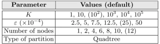
Parameter Values (default)

K 1, 10, (102), 103, 104, 105

ε(×10−4

) 2.5, 5, 7.5, 12.5, (25), 50 Number of nodes 1, 2, 4, 6, 8, 10, (12) Type of partition Quadtree

Table 1.Configuration parameters used in the experiments.

Table 1 summarizes the configuration parameters used in our experiments. Default values (in parentheses) are used unless otherwise mentioned. Spatial-Hadoop needs the datasets to be partitioned and indexed before invoking the spatial operations. The times needed for that pre-processing phase are 94 secs for LAKES, 103 sec for P ARKS, 175 sec for BU ILDIN GS and 200 sec for

CLU S LAKES. We have shown the time of this pre-processing phase in Spati-alHadoop (disk-based DSDMS), since it would be the full execution time, at least in the first running of the query. Note that, data are indexed and the index is stored on HDFS and for subsequent spatial queries, data and index are already available (this can be considered as an advantage of SpatialHadoop). On the other hand, LocationSpark (in-memory-based DSDMS) always partitions and indexes the data for every operation. The partitions/indexes are not stored on any persistent file system and cannot be reused in subsequent operations.

3 _{Available athttp://spatialhadoop.cs.umn.edu/datasets.html} 4

Available athttps://github.com/aseldawy/spatialhadoop2 5

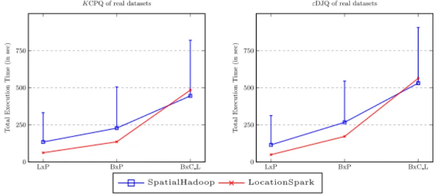
Our first experiment aims to measure the scalability of theKCPQ andεDJQ algorithms, varying the dataset sizes. As shown in the left chart of Figure 4 for the KCPQ of real datasets (LAKES×P ARKS, BU ILDIN GS ×P ARKS

and BU ILDIN GS×CLU S LAKES), the execution times in both DSDMSs increase linearly as the size of the datasets increase. Moreover, LocationSpark is faster for all the datasets combinations except for the largest one (e.g. it is 29 sec slower for the biggest datasets,BU ILDIN GS×CLU S LAKES(BxC L)). However, it should be noted that SpatialHadoop needs a pre-indexing time of 175 and 200 sec for each dataset (depicted by vertical lines in the charts) and that difference can be caused by memory constraints on the cluster.

As we have just seen forKCPQ, the behavior of the execution times when varying the size of the datasets is very similar for εDJQ. For instance, for the combination of large datasets (see the right chart of Figure 4),BU ILDIN GS× CLU S LAKES (BxC L), SpatialHadoop is 32 sec faster than LocationSpark. However, for smaller sets, LocationSpark shows better performance (e.g. it is 96 sec faster for the middle size datasets,BU ILDIN GS×P ARKS (BxP)). From these results with real data, we can conclude that both DSDMSs have similar performance, in terms of execution time, even showing LocationSpark better values in most of the cases, despite the fact that neither pre-partitioning nor pre-indexing are done.

LxP BxP BxC L 0 250 500 750 T otal Execution Time (in sec) KCPQ of real datasets LxP BxP BxC L 0 250 500 750 T otal Execution Time (in sec) εDJQ of real datasets SpatialHadoop LocationSpark

Fig. 4.KCPQ (left) andεDJQ (right) execution times considering different datasets. The second experiment studies the effect of the increasing bothKandεvalue for the combination of the biggest datasets (BU ILDIN GS×CLU S LAKES). The left chart of Figure 5 shows that the total execution time for real data-sets grows slowly as the number of results to be obtained (K) increases. Both DSDMSs, employing Quadtree, report stable execution times, even for largeK

values (e.g. K= 105_{). This means that the Quadtree is less affected by the} in-crement of K, because Quadtree employs regular space partitioning depending on the concentration of the points. As shown in the right chart of Figure 5, the total execution time grows as theεvalue increases. Both DSDMSs (SpatialHa-doop and LocationSpark) have similar relative performance for allεvalues, with SpatialHadoop being faster, except forε= 50×10−4_{, where LocationSpark}

out-performs it (i.e. LocationSpark is 377 sec faster). This difference is due to the way in which εDJQ is calculated in the latter, where fewer points are used as candidates and skew cells are dealt with itsQuery Plan Scheduler. For smaller

ε values SpatialHadoop preindexing phase reduces time considerably for very large datasets.

The main conclusions that we can extract for this experiment are: (1) the higherKorεvalues, the greater the possibility that pairs of candidates are not pruned, more tasks would be needed and more total execution time is consumed and, (2) LocationSpark shows better performance especially for higher values of

K andε thanks to its Query Plan Scheduler and the reduction of the number of candidates. 1 10 102 103 104 105 0 500 1,000 1,500 K: # of closest pairs T otal Execution Time (in sec) BUILDINGSxCLUS LAKES -KCPQ 2.5 5 7.5 12.5 25 50 0 500 1,000 1,500

ε: distance threshold values (×10−4₎

T otal Execution Time (in sec) BUILDINGSxCLUS LAKES -εDJQ SpatialHadoop LocationSpark

Fig. 5. KCPQ cost (execution time) vs. K values (left) and εDJQ cost (execution time) vs.εvalues (right).

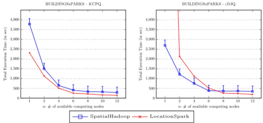
The third experiment aims to measure the speedup of the DJQ MapReduce algorithms (KCPQ andεDJQ), varying the number of computing nodes (n). The left chart of Figure 6 shows the impact of different number of computing nodes on the performance of parallelKCPQ algorithm, forBU ILDIN GS×P ARKS

with the default configuration values. From this chart, it could be concluded that the performance of our approach has direct relationship with the number of computing nodes. It could also be deduced that better performance would be obtained if more computing nodes are added. LocationSpark is still showing a better behavior than SpatialHadoop. In the right chart of Figure 6, we can observe a similar trend forεDJQ MapReduce algorithm with less execution time, but in this case LocationSpark shows worse performance for a smaller number of nodes. This is due to the fact that LocationSpark and εDJQ depends more on the available memory and when the number of nodes decreases, this memory also decreases considerably.

By analyzing the previous experimental results, we can extract several con-clusions that are shown below:

– We have experimentally demonstrated theefficiency (in terms of total exe-cution time) and thescalability(in terms ofKandεvalues, sizes of datasets

1 2 4 6 8 10 12 0 500 1,000 1,500 2,000 2,500 3,000 3,500 4,000

n: # of available computing nodes

T otal Execution Time (in sec) BUILDINGSxPARKS -KCPQ 1 2 4 6 8 10 12 0 500 1,000 1,500 2,000 2,500 3,000 3,500 4,000

n: # of available computing nodes

T otal Execution Time (in sec) BUILDINGSxPARKS -εDJQ SpatialHadoop LocationSpark

Fig. 6.Query cost with respect to the number of computing nodesn.

and number of computing nodes (n)) of the proposed parallel algorithms for DJQs (KCPQ andεDJQ) in SpatialHadoop and LocationSpark.

– The larger theKor εvalues, the larger the probability that pairs of candi-dates are not pruned, more tasks will be needed and more total execution time is consumed for reporting the final result.

– The larger the number of computing nodes (n), the faster the DJQ algo-rithms are.

– Both DSDMSs have similar performance, in terms of execution time, alt-hough LocationSpark shows better values in most of the cases (if an adequate number of processing nodes with adequate memory resources are provided), despite the fact that neither pre-partitioning nor pre-indexing are done.

6

Conclusions and Future Work

The KCPQ andεDJQ are spatial operations widely adopted by many spatial and GIS applications. These spatial queries have been actively studied in cen-tralized environments, however, for parallel and distributed frameworks has not attracted similar attention. For this reason, in this paper, we compare two of the most current and leading DSDMSs, namely SpatialHadoop and LocationSpark. To do this, we have proposed novel algorithms in LocationSpark, the first ones in literature, to perform efficient parallel and distributedKCPQ andεDJQ al-gorithms on big spatial real-world datasets, adopting the plane-sweep technique. The execution of a set of experiments has demonstrated that LocationSpark is the overall winner for the execution time, due to the efficiency of in-memory pro-cessing provided by Spark and additional improvements as theQuery Plan Sche-duler. However, SpatialHadoop is a more mature and robust DSDMS because of time dedicated to investigate and develop it (several years) and, it provides more spatial operations and spatial partitioning techniques. Future work might cover studying other Spark-based DSDMSs like Simba [14], implement other spatial partitioning techniques [4] in LocationSpark and, design and implement other DJQs in these DSDMSs for further comparison.

References

1. A. Aji, F. Wang, H. Vo, R. Lee, Q. Liu, X. Zhang and J.H. Saltz: “Hadoop-GIS: A high performance spatial data warehousing system over MapReduce”,PVLDB 6(11): 1009-1020, 2013.

2. A. Corral, Y. Manolopoulos, Y. Theodoridis and M. Vassilakopoulos: “Algorithms for processingK-closest-pair queries in spatial databases”,Data Knowl. Eng.49(1): 67-104, 2004.

3. J. Dean and S. Ghemawat: “MapReduce: Simplified data processing on large clus-ters”,OSDI Conference, pp. 137-150, 2004.

4. A. Eldawy, L. Alarabi and M.F. Mokbel: “Spatial partitioning techniques in Spa-tialHadoop”,PVLDB8(12): 1602-1613, 2015.

5. A. Eldawy, Y. Li, M.F. Mokbel and R. Janardan: “CG Hadoop: computational geometry in MapReduce”,SIGSPATIAL Conference, pp. 284-293, 2013.

6. A. Eldawy and M.F. Mokbel: “SpatialHadoop: A MapReduce framework for spatial data”,ICDE Conference, pp. 1352-1363, 2015.

7. F. Garc´ıa, A. Corral, L. Iribarne, M. Vassilakopoulos and Y. Manolopoulos: “En-hancing SpatialHadoop with Closest Pair Queries”,ADBIS Conference, pp. 212-225, 2016.

8. R.K. Lenka, R.K. Barik, N. Gupta, S.M. Ali, A. Rath and H. Dubey: “Compara-tive Analysis of SpatialHadoop and GeoSpark for Geospatial Big Data Analytics”, CoRRabs/1612.07433, 2016.

9. F. Li, B.C. Ooi, M.T. ¨Ozsu and S. Wu: “Distributed data management using MapReduce”,ACM Comput. Surv.46(3): 31:1-31:42, 2014.

10. G. Roumelis, A. Corral, M. Vassilakopoulos and Y. Manolopoulos: “New plane-sweep algorithms for distance-based join queries in spatial databases”, GeoInfor-matica20(4): 571-628, 2016.

11. J. Shi, Y. Qiu, U.F. Minhas, L. Jiao, C. Wang, B. Reinwald and F. ¨Ozcan: “Clash of the Titans: MapReduce vs. Spark for Large Scale Data Analytics”, PVLDB 8(13): 2110-2121, 2015.

12. M. Tang, Y. Yu, Q.M. Malluhi, M. Ouzzani and W.G. Aref: “LocationSpark: A Distributed In-Memory Data Management System for Big Spatial Data”,PVLDB 9(13): 1565-1568, 2016.

13. M. Tang, Y. Yu, W.G. Aref, A.R. Mahmood, Q.M. Malluhi and M. Ouzzani: “In-memory Distributed Spatial Query Processing and Optimization”, Available at: http://merlintang.github.io/paper/memory-distributed-spatial.pdf, April, 2017. 14. D. Xie, F. Li, B. Yao, G. Li, L. Zhou and M. Guo: “Simba: Efficient In-Memory

Spatial Analytics”,SIGMOD Conference, pp. 1071-1085, 2016.

15. S. You, J. Zhang and L. Gruenwald: “Large-scale spatial join query processing in cloud”,ICDE Workshops, pp. 34-41, 2015.

16. S. You, J. Zhang and L. Gruenwald: “Spatial join query processing in cloud: Analy-zing design choices and performance comparisons”,ICPPW Conference, pp. 90-97, 2015.

17. J. Yu, J. Wu and M. Sarwat: “GeoSpark: a cluster computing framework for pro-cessing large-scale spatial data”,SIGSPATIAL Conference, pp. 70:1-70:4, 2015. 18. M. Zaharia, M. Chowdhury, T. Das, A. Dave, J. Ma, M. McCauly, M.J. Franklin,

S. Shenker and I. Stoica: “Resilient Distributed Datasets: A Fault-Tolerant Ab-straction for In-Memory Cluster Computing”,NSDI Conference, pp. 15-28, 2012. 19. H. Zhang, G. Chen, B.C. Ooi, K.-L. Tan and M. Zhang: “In-Memory Big Data