Workload Scheduling in Distributed Stream Processors using Graph Partitioning

Zurich Open Repository and Archive University of Zurich Main Library Strickhofstrasse 39 CH-8057 Zurich www.zora.uzh.ch Year: 2015

Workload Scheduling in Distributed Stream Processors using Graph

Partitioning

Fischer, Lorenz ; Bernstein, Abraham

Abstract: With ever increasing data volumes, large compute clusters that process data in a distributed manner have become prevalent in industry. For distributed stream processing platforms (such as Storm) the question of how to distribute workload to available machines, has important implications for the overall performance of the system. We present a workload scheduling strategy that is based on a graph partitioning algorithm. The scheduler is application agnostic: it collects the communication behavior of running applications and creates the schedules by partitioning the result- ing communication graph using the METIS graph partitioning software. As we build upon graph partitioning algorithms that have been shown to scale to very large graphs, our approach can cope with topologies with millions of tasks. While the experiments in this paper assume static data loads, our approach could also be used in a dynamic setting. We implemented our proposed algorithm for the Storm stream processing system and evaluated it on a commodity cluster with up to 80 machines. The evaluation was conducted on four different use cases – three using synthetic data loads and one application that processes real data. We compared our algorithm against two state-of-the-art sched- uler implementations and show that our approach offers sig-nificant improvements in terms of resource utilization, enabling higher throughput at reduced network loads. We show that these improvements can be achieved while maintaining a balanced workload in terms of CPU usage and bandwidth consumption across the cluster. We also found that the performance advantage increases with message size, providing an important insight for stream-processing approaches based on micro-batching.

DOI: https://doi.org/10.1109/BigData.2015.7363749

Posted at the Zurich Open Repository and Archive, University of Zurich ZORA URL: https://doi.org/10.5167/uzh-120510

Conference or Workshop Item Accepted Version

Originally published at:

Fischer, Lorenz; Bernstein, Abraham (2015). Workload Scheduling in Distributed Stream Processors using Graph Partitioning. In: 2015 IEEE International Conference on Big Data (IEEE BigData 2015), Santa Clara, CA, USA, 29 October 2015 - 1 November 2015.

Workload Scheduling in Distributed Stream

Processors using Graph Partitioning

Lorenz Fischer

Abraham Bernstein

Abstract—With ever increasing data volumes, large compute clusters that process data in a distributed manner have become prevalent in industry. For distributed stream processing platforms (such as Storm) the question of how to distribute workload to available machines, has important implications for the overall performance of the system.

We present a workload scheduling strategy that is based on a graph partitioning algorithm. The scheduler is application agnostic: it collects the communication behavior of running applications and creates the schedules by partitioning the result-ing communication graph usresult-ing the METIS graph partitionresult-ing software. As we build upon graph partitioning algorithms that have been shown to scale to very large graphs, our approach can cope with topologies with millions of tasks. While the experiments in this paper assume static data loads, our approach could also be used in a dynamic setting.

We implemented our proposed algorithm for the Storm stream processing system and evaluated it on a commodity cluster with up to 80 machines. The evaluation was conducted on four different use cases – three using synthetic data loads and one application that processes real data.

We compared our algorithm against two state-of-the-art sched-uler implementations and show that our approach offers sig-nificant improvements in terms of resource utilization, enabling higher throughput at reduced network loads. We show that these improvements can be achieved while maintaining a balanced workload in terms of CPU usage and bandwidth consumption across the cluster. We also found that the performance advantage increases with message size, providing an important insight for stream-processing approaches based on micro-batching.

I. INTRODUCTION

When work has to be distributed across a compute cluster, scheduling—the process of deciding which cluster machine is assigned which part of the workload—is of paramount importance for the overall performance of the system. Exten-sive research has been conducted in the realm of scheduling work in data-parallel systems. In data-parallel systems, data is partitioned into small units, which are then assigned to worker nodes in a compute cluster to process. A prominent representative of data-parallel systems is Apache Hadoop1 which is the most popular implementation of MapReduce [1]. Rao and Reddy [2] give an overview over several scheduling strategies within the Hadoop MapReduce framework such as FiFo, fair, capacity, delay, deadline, and resource-aware schedulers.

1_{http://hadoop.apache.org}

In contrast to data-parallel systems, task-parallel appli-cations are designed as a set of tasks that run in parallel on a cluster for indefinite time. While these systems also incorporate data-parallism, the processing is divided across the cluster and the data is partitioned and routed to task instances, accordingly. Google’s Millwheel [3], Microsoft’s Naiad [4] and Timestream [5], IBM’s Infosphere Streams [6], as well as Apache Storm2_{are representatives of such systems.}

Workload schedulers of task-parallel systems need to distribute the compute tasks in a way that makes optimal use of the available compute resources.

In this study, we present a workload scheduler for task-based distributed stream processing systems that is task-based on a graph partitioning algorithm. We implemented the scheduler for the Apache Storm platform and measured its performance in an extensive empirical evaluation. This work is a continua-tion of ideas presented at a workshop where we first proposed building a Storm scheduler based on graph partitioning [7]. While this previous work was based on simulations, the study at hand presents an evaluation on actual compute clusters in a real world setup. In particular the contributions of this study are as follows:

1) We present an implementation of a scheduling al-gorithm to schedule operators in a distributed task-parallel stream processing system which is based on graph partitioning.

2) We present a set of benchmark topologies with their associated data to evaluate our scheduler on the Storm realtime processing framework.

3) We evaluate our algorithm against two alternative approaches in an extensive evaluation on a wide range of varying cluster configurations.

4) We report on key lessons learned and discuss the implications of our observations for the field of distributed stream processing.

The remainder of this paper is organized as follows: We give an overview of related work in Section II, before introducing our algorithm in Section III. We then present the experimental setup and our results in Sections IV and V, respectively. We close with a discussion of our findings in Section VI.

II. RELATEDWORK

Our work is related to the fields of workload scheduling in distributed systems as well as using graph partitioning algorithms for resource allocation. Here we succinctly report on related work in these fields and discuss our research in its light.

A. Workload Scheduling in Distributed Systems

Most research in workload scheduling for distributed sys-tems has been conducted for batch-based syssys-tems. In such systems data is partitioned into small shards that are then assigned to worker nodes. [2] reviews common scheduling strategies for data-parallel systems. We only mention Sparrow [8] here, because its application is a low latency data-parallel system that could be used in a streaming setup. Sparrow is a low latency task scheduler for data-parallel systems based on a decentralized randomized sampling approach that has been evaluated in the Spark [9] environment. It continuously assigns tasks of processing small batches of data based on local information to minimize the delay in job execution. The overarching goal of this work is to achieve low latency in scheduling. Our study focuses on task-parallel processing [6], where the overall system performance in terms of throughput and network utilization takes precedence over the latency of scheduling a single computation.

In contrast to batch-based distributed systems, where scheduling speed can become an issue, in a task-based environ-ments, workload assignments can persist for longer durations. One early representative of a task-based processing is Borealis [10], which places operators of a streaming system across geographically distributed computers. Pietzuch et al. presented their scheduler that is based on astream-based overlay network

(SBON) optimizing operator placement [11]. Xing et al. pre-sented two different scheduling approaches for the Borealis System. In [12] they propose a greedy heuristic to find an optimal operator placement in polynomial time and in [13] they propose to find an operator placement that is “resilient” to change, meaning that it does not have to be changed upon load changes. Heinze et al. model the problem of operator placement in Borealis as a bin-packing problem and use a firstfit heuristic to assign operators to machines (bins) [14].

Other task-based systems distribute work across a set of computers within the same data center. For example, Isard et al. presented a scheduling system for Microsoft’s Dryad [15] in [16]. This scheduler maps the problem of task to worker assignment into a graph over which a min-cost flow algorithm then minimizes the cost of a model which includes data locality, fairness, and starvation-freedom. Wolf et al. presented the scheduling system SODA [17], which is the workload scheduling system of System S (later renamed to IBM In-fosphere Streams). In SODA, the assignment of processing elements (PE) to cluster nodes is usually handled by a mixed integer program implemented in CPLEX3_{to balance CPU and}

bandwidth constraints. When the mixed integer program fails, due to the quadratic complexity of the problem, then either round-robin or a heuristics-based scheduling mechanism is used. The former essentially corresponds to Storm’s default

3_{http://www-01.ibm.com/software/commerce/optimization/cplex-optimizer}

scheduling strategy. The latter tries to assigns all communicat-ing PE pairs to the same machine incrementally startcommunicat-ing from the pair that communicates most.

Aniello et al. [18] present two scheduling algorithms for Storm. Theirofflinescheduler bases its work assignments on an analysis of the topology of the program, theironlinescheduler takes runtime CPU and network load characteristics of the cluster into account following a procedure conceptually similar to heuristic module employed by SODA: all communicating processing pairs of Storm tasks (Storm’s equivalent of a PE) are sorted according to the amount of communication between them and assigned to worker nodes on a best-effort basis.

In Naiad [4], one shard of each operator is assigned to each worker4_{, a strategy that for certain configurations is equivalent}

to the default scheduler of Storm.

Finally, two query planning systems need to be mentioned: in StreamCloud [19], information contained in the query is leveraged to do the scheduling. Hence, each operator that is used in the query needs to have a counter part in the scheduler. As inter-operator communication is handled in the query com-piler, StreamCloud’s greedy load balancing (scheduling) algo-rithm focuses on machine load in terms of CPU. Kalyvianaki et al. present an approach that solves the N P-hard multi-query planning problem by cleverly approximating an optimal placement [20]: in their SQPR planner, they incrementally add queries to the cluster, trying to re-use parts of existing queries where possible. In contrast to these works, the approach taken by Storm is to separate the task of scheduling from the query compiler, which allows arbitrary code to run in the operators. Our approach differs from the above-mentioned schedulers in that we employ a graph partitioning algorithm of the METIS software package [21]. In contrast to a min-flow approach, we consider both network and machine load. Our approach differs from SODA’s mixed integer program in that we use graph partitioning algorithms that have been shown to scale to millions of edges, using heuristics to avoid the complexity constraints [21]. Hence, our investigation will compare to the round-robin base-line and Aniello’s on-line algorithm that is conceptually similar to the latter of SODA’s heuristics.

B. Graph Partitioning for Scheduling

Others have employed graph partitioning algorithms to the problem of workload scheduling before us: Alet´a et al. [22] use graph partitioning algorithms to assign instructions to different clusters inside a microprocessor. Similar to our use-case, their goal is to group instructions/operations into clusters in order to balance the workload whilst minimizing inter-cluster communication. Curino et al. use METIS for database replication [23]: They map tuples in the database as nodes and transactions as edges of a graph and let METIS figure out an optimal replication strategy. [24] gives a survey of other applications including “VLSI circuit layout, image pro-cessing, solving sparse linear systems, computing fill-reducing orderings for sparse matrices, and distributing workloads for parallel computations.” Lastly, and most closely related to our application, graph partitioning has even been applied in

4

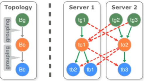
Server 1 Server 2 to1 tb1 tb2 to2 tb3 tg1 tg2 tg3 Topology Bo Bb Bg grouping grouping

Fig. 1. Logical (left) and physical (right) representation of a topology

stream processing in System S. Their offline compiler uses a graph partitioner to fuse multiple processing elements (PEs) of a stream processing graph into bigger PEs in order to decrease inter-process communication [25]. In contrast,we use

information that we collected in an onlinephase to inform

just-in-time re-scheduling of the workload in the running system. Hence, we can exploit actual run-time information such as actual computational effort and network usage to optimize our schedule.

III. SCHEDULINGALGORITHM

In this section, we will describe our approach. We will first give more details about Storm. Then we formally describe how we map the problem of workload scheduling into a graph partitioning problem.

A. Distributed Stream Processing with Storm

In contrast to batch-based distributed systems such as Apache MapReduce,5 Storm6 ingests data continuously. As in MapReduce, a Storm application allows the user to partition the data and to distribute parts of the processing across a compute cluster.

A Storm application—a topology—is a directed graph consisting of spout and bolt nodes as the one depicted in Figure 1 on the left. Spouts emit data and bolts consume data from upstream nodes and emit data to downstream nodes. Spout nodes are typically used to connect a Storm topology to external data sources such as queues, web-services, or file systems. For each spout and bolt, the programmer defines how many instances of this node should be created in the physical instantiation of the topology – the task instances. These task instances, or tasks, are distributed across all machines of the compute cluster, to which a topology has been assigned. Each edge in the topology graph defines a grouping strategy

according to which messages that pass between the nodes—

the tuples—are sent to downstream nodes. This results in a

physical topology depicted on the right of Figure 1, which is different than the logical representation.

Tuples are lists of key-value pairs. The program-mer defines the tuple format for each edge of the topology (e.g. field1=query terms, field2=browser cookie, field3=timestamp). Different grouping strategies provide dif-ferent guarantees. For example, the field grouping strategy guarantees, that all tuples that share the same value in one or multiple configurable fields are sent to the same task instance. In order to provide reliability guarantees, Storm offers an “acking” (acknowledgment) facility that makes sure that each

5_{http://hadoop.apache.org} 6_{https://storm.apache.org}

tuple is successfully processed at least once. When a spout emits a tuple, it attaches an id to the outgoing tuple and will be informed by the framework, as soon as a tuple has been fully processed by all downstream bolts. In the case of errors, Storm informs the emitting spout of any tuples that failed to be processed, so it can re-emit these tuples.

In contrast to MapReduce, where processing is moved to the data, Storm has no inherent data locality as streaming data is ingested from external sources. However, processing can be arranged in a way that reduces the amount of network load incurred by the system due to data movement while still making good use of the compute resources that are available. This process is called scheduling.

B. Workload Partitioning and Scheduling in Storm

For topology edges that have a field grouping configured, Storm guarantees that all tuples that share the same value(s) for one or multiple fields, are processed by the same task instance of the bolt. To that end it hashes the field’s values to an integer and uses the modulo function to assign a given tuple to a task instance of the receiving bolt.

As an example, consider the topology depicted in Figure 1: Whenever one of the task instances of boltBoemits a tuple, the value of the field configured in the field grouping strategy is hashed, its modulo 3 is computed, and the tuple is then sent to the task instance ofBbwith the corresponding number (tb1,tb2, ortb3). We compute modulo 3 as the receiving bolt

Bb has been configured with a degree of parallelism of 3. If there are multiple bolts in a row that all expect their input data grouped on the same field, it will be prudent to place the corresponding task instances on the same cluster machine, so that the communication overhead between the two task instances can be reduced to the passing of a pointer to an object in memory. Assuming that a storm topology keeps most of its data in memory, the topology’s throughput bottleneck, therefore, is the amount of network traffic necessary to process the data. As Storm’s decision of where to send a data tuple to depends on the contents of the tuples passed within the running topology, the actual communication behavior between the task instances can only be measured at runtime (or with highly specific knowledge about the data distributions that is typically not available ex ante). The communication behavior of a running topology can be thought of as a weighted directed graph, in which the weights on the nodes represent the compute resources that a task instance needs to process and the weights on the edges represent the accumulated size of all the tuples that are sent from one task to the next. We refer to this graph as the topology’scommunication graph. We describe this more formally in the next section.

C. Graph Partitioning for Scheduling in Storm

In the following paragraphs we will formally describe how we map the problem of workload scheduling in Storm to a graph partitioning problem.

1) The Communication Graph: The logical view of a Storm

topology can be understood as a graphT = (B, C), where B

is a finite set of bolts and spouts connected by a finite set of connections C⊂B×B. Each boltbi ∈B is configured with

a degree of parallelism dpi ∈ N. Each connection ci ∈ C is configured with a grouping strategy gi∈G.

The physical view of a Storm topology is again a graph

G= (V, E). Each bolt and spout bi ∈B is represented by a set of task instancesVi∈V where|Vi|=dpi. Any two sets of vertices VxandVy are connected through at most|Vx| × |Vy| vertices. The graph is weighted. The vertex weights vwi ∈

R>0represent the amount of compute resources consumed by task instancevi∈Vi. The edge weightsewij∈R>0represent the amount of information exchanged between the two task instancesvi andvj.

2) Graph Partitioning: A partitioning divides a set into

pairwise disjoint sets. In our case we want to partition the vertices V of a graph G into a set of K partitions. A partitioning P = {P1, . . . , PK} for V separates the set of vertices such that

• it covers the whole set of vertices:SK_k=1Pk=V and

• the partitionsPk are pairwise disjoint: TK_k=1Pk =∅

In addition, we denote (i) a partitioning function by part : V →Pthat assigns every vertexvito a partitionPk ∈P, (ii) a

cost functionbycost(G, P)∈_R, which denotes some kind of

cost associated with the partitioning P of the communication graph G that is subject to optimization, and (iii) a load

imbalance factorloadImba(G, P)∈R>0that ensures that the

workload of the tasks is evenly distributed over the machines. We can now map our problem of minimizing the number of messages that are sent between machines to a graph partitioning problem with a specific cost function. First, we define the graph to be partitioned as the communication graph

G and we set K to be equal to be the number of machines in our cluster. A partitioning of G maps each task instance (vi ∈ V) to exactly one machine. Second, we define a cost function for a partitioning P of a communication graphGas

cost(G, P) = V X i=1 V X j=1 differentPart(i, j)∗ewij

where the function differentPart(i, j)is defined as

differentPart(i, j) =

1 part(vi)6=part(vj)

0 otherwise

Third, when optimizing the costs for the partitions we add the constraint that the partitions shall be balanced with respect to the computational load. More precisely, we define a load imbalance factor as

loadImba(G, P) =max(pwk/apw)

wherepwk is the summed weights of all vertices in partition

k andapw is the average partition weight over all partitions of partitioning P.

In order to minimize the amount of network communica-tion within a running Storm topology, the following optimiza-tion problem has to be solved:

minimize

x cost(G, P)

subject to loadImba(G, P)≤I

whereIis a the maximum imbalance we are willing to accept. The communication graph is constructed as follows: In-stead of computing the object size of each tuple, we approx-imate the communication load by counting the messages that that are emitted from any spout or bolt task instance. These counts are then used as a proxy for the edge weight between the sending and the receiving task instance. Assuming that each tuple that is either emitted from or received by a task instance will also incur some processing load, we sum the number of all emitted and all received tuples and use this value as the node weight in the communication graph.

All graph partitionings in this paper were computed using the METIS algorithms for graph partitioning [21] – a well established graph partitioning package.

IV. EXPERIMENTALDESIGN

In the following paragraphs we are going to present the design of our experiments. We first list the metrics we collected to measure the performance of the systems. We then present the schedulers we evaluated and the topologies we used to measure their performance. Lastly, we present the cluster setup used.

A. Performance Metrics

A good stream scheduler maximizes the throughput of a system whilst minimizing the system load. We operationalize these measures as follows:

1) Throughput: As a streaming system runs continuously,

we measured throughput as the number of tuples that all spouts of a topology emit per second. We averaged this value over the whole runtime of a test run.

2) Bandwidth: The most constraining bottleneck in a

dis-tributed streaming system is the the network that connects cluster nodes. As such, we measured the number of bytes that were transferred over network interfaces of the cluster machines during our experiments.

Note that we do not consider CPU load to be a constraining factor as we assume that more machines can be added to a cluster to accommodate increased load requirements. In such scenarios, internode-communication is often the principle performance bottleneck [26].

B. The Schedulers

1) Default / Even Scheduler: The default scheduler shipped

with Storm is calledEven Scheduler7. It evenly assigns all task instances to the available worker nodes and does not take any performance metrics of the running topology into account. In this paper, we refer to this scheduler as the “Default” scheduler.

2) Greedy Scheduler: Aniello et al. present two different

schedulers as an alternative to the Default scheduler provided by storm in their paper in [18]. The first scheduler analyses the topologies offline and bases its scheduling decision on this offline analysis. The second scheduler they propose is a traffic-based online scheduler which takes performance metrics

7

of the running topologies into account. The online scheduler implements a “greedy heuristic” that tries to compute an optimal schedule at runtime. As the latter outperformed the former in all experiments, we only compare with the traffic-based version and refer to this scheduler as the “Greedy” scheduler. We will outline this scheduler in the paragraphs below and refer to [18] for a more detailed description.

As with our graph partitioning based scheduler, the Greedy scheduler is built around the idea of using collected perfor-mance statistics of a running topology to compute the optimal workload distribution in the cluster. Similar to our approach, information about the sending behavior of running tasks is collected. Additionally, information about how much time the threads of each task spend executing code is collected. In combination with the clock rate of the CPU, the Greedy scheduler also tries to recognize and react to system overload of compute nodes.

The algorithm works as follows: First, all task instance pairs of a running topology are sorted in descending order according to the number of messages passed between the pairs. Then, the algorithm iterates over the pairs, trying to co-locate task instances that have high communication volumes. If this co-location is not possible, because it would result in overloading one of the workers, there are nine different co-location combinations that are investigated to find the most optimal placement. An analogous strategy is then used to distribute workers across the supervisors.

We used the version of the Greedy scheduler that we downloaded from the linked sources in [18]. This version reacts to two different states that can trigger the re-scheduling process. First, scheduling can trigger when the previously computed schedule would result in an inter-machine traffic that would be lower than a certain percentage of the old schedule. This percentage value is configurable and for our experiments, has been set to 1%, meaning that we would always fire if there are traffic benefits to be expected. Second, scheduling of a topology can be triggered when any of the cluster machines is overloaded in terms of CPU usage. The data is collected and aggregated over windows and the scheduler does not schedule more often than every reschedule.timeout seconds. For our experiments we set this value to 1 minute. The sensitivity that the scheduler shows towards load imbalances can be configured using three parameters alf a, beta, and gamma, for which we used the values found in [18].8

The implementation of the Greedy scheduler we down-loaded only works for spouts and bolts that have been (man-ually) registered. As several of Storm’s internal services are based on bolts that do not contain this registration code, this implementation did not assign all task instances during the scheduling process. For this reason, we implemented a fix that evenly distributes all unassigned task instances across all workers of the cluster. These modifications, along with all the source code used for this paper, can be downloaded from https://github.com/lorenzfischer/storm-scheduler.

3) Metis Scheduler: In order to test our proposed

schedul-ing algorithm, we leveraged the graph partitionschedul-ing software METIS [21]: we first use the metrics collection framework of

8_{alf a= 0.0, beta= 0.5, gamma= 1.1}

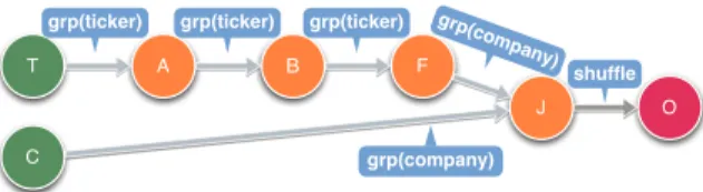
A T O C B F J grp(company) shuffle grp(ticker) grp(ticker) grp(ticker) grp(c

ompa_ny)

Fig. 2. OpenGov topology, joining ticker data (T) with public contracts (C)

Storm to collect the communication graph data at runtime. At a configurable timeout, the resulting graph is partitioned using METIS and the partitioning used as the workload schedule. We set this timeout value to always be the same as the correspond-ing timeout value of the Greedy scheduler. Note that in this paper, scheduling only happens once per evaluation run at the specified timeout. To create the schedule, we used thegpmetis

program in its standard configuration, which creates partitions of equal size, and only changed the -objtype parameter to instruct METIS to optimize for total communication volume when partitioning, rather than minimizing on total edgecut. We used Metis version 5.1.0 with default partitioning (kway) and default load imbalance of 1.03. The strategy METIS uses, to compute good partitionings fast, is multilevel graph bisection: it incrementally coarsens the graph by collapsing nodes and edges to arrive at a smaller version of the graph. It then partitions this smaller graph, before it uncoarsens the graph into its original form, adapting the partitioning at each uncoarsening step to account for the newly un-collapsed vertices and edges. In this paper, we refer to this scheduler as the “Metis scheduler.”

C. Topologies

We tested all three schedulers using four different topology implementations. In the following paragraphs each topology will be motivated and explained in detail.

1) OpenGov Topology: The first topology represents a

query over two realworld data sources which combines data on public spending in the US with stock ticker data.9We devised a query that would highlight (publicly traded) companies, that double their stock price within 20 days and are/were awarded a government contract in the same time-frame. The query requires the system to scan the two sources, aggregate/filter values, and finally join certain events that may have a causal relation to each using a temporal condition.

The resulting topology (Figure 2) first aggregates (A) the ticker-sourced (T) data to compute the minimum and maximum value over a time window of 20 days. It computes the ratio between these numbers (B) and then filters those solutions, where that ratio is smaller than or equal to two (F). The remaining company tickers are then joined (J10_{) with the}

ones that where awarded government contracts (C). The joined tuples are then sent to the output node (O). The spout nodes (T and C) read the data form HDFS and the output bolt (O) writes the results back to HDFS.

When varying the cluster size, we set the parallelism for all bolts to be equal to the number of cluster machines of the test. For the spouts, we chose the combined number to be equal to the number of cluster machines and partitioned the

9_{http://www.usaspending.gov, https://wrds-web.wharton.upenn.edu/wrds} 10_{We use a hash join with eviction rules for the temporal constraints.}

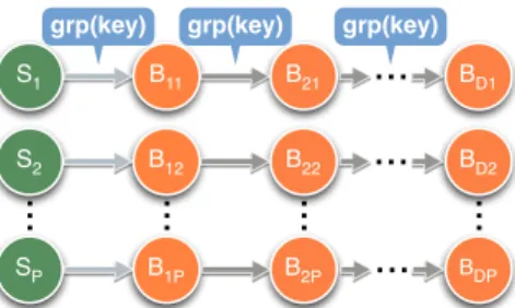
B₁₁ B₂₁ S₁ grp(key)

...

...

...

...

...

...

...

Fig. 3. Physical instantiation ofParallelandPayloadtopologies

data accordingly. The output was always sent to one single output task, so the output bolt had a degree of parallelism of one. For example, in the case of a 10 machine cluster, we configured a degree of parallelism of 10 for all bolts but the output bolt and had 5 input files for the contract and the ticker source, respectively. This setup amounts to 6 tasks for each worker machine.11

2) Parallel Topology: The idea behind this topology was to

develop a topology that would be trivial to distribute across the cluster. One way to achieve this, is to have several independent (embarassingly parallel) messaging channels: The “Parallel” topology reflects this setup. The physical instantiation of the topology is shown in Figure 3: The topology consists of one spout and a number of D (depth) bolts that are all serially connected. The tuples passing between the nodes in the topology are identical throughout the topology and consist of a single 128-bit MD5 hash value which is generated in the spout. The degree of parallelism (P) is defined for the whole topology and defines how many instances of each spout/bolt will be instantiated in the running topology.

To keep the communication between the bolts in straight lines, each spout generates a key value that will always be routed to the same bolt instance when sent over an edge configured with the field-grouping strategy. Whenever a bolt receives a tuple, it emits a new tuple that contains the key value of the received tuple before acknowledging the received tuple. As the bolts are also connected to each other using field-grouped edges, each bolt task emits values that are routed to exactly one other bolt. This setup results in a quadraticD×P

topology instantiation. Assuming that one worker node in the cluster is capable of runningD+1 tasks, the optimal workload scheduling in this topology would be to put all D bolt tasks together with their spout task on one machine and do the same for all otherP groups.

To prevent our bandwidth measurements to be influenced from waiting threads on overloaded worker nodes, we empir-ically tested how many task instances can be assigned to one worker machine without the worker being overloaded. Figure 4 shows the throughput values achieved on one worker machine running varying numbers of tasks. We note that while running fewer than 8 tasks is underutilizing the available resources, running more than 12 tasks yields no further increase in throughput. As our topologies need to run several statistics collection routines, we kept the number of tasks running on any single worker machine around 8. For this reason we chose

D = 7, meaning that we ran 8 task instances per machine (1 spout task and 7 bolt tasks). When we varied the cluster size, we always set the value ofP to be the same as the number of

11_{Plus one spare output bolt task.}

8 10 12 2 4 6 8 10 12 14 16 Tasks Mio Tuples

Fig. 4. Throughput achieved by varying the number of tasks on one cluster machine transmitting tuples of size 3KB.

workers.

3) Payload Topology: As we anticipated the bookkeeping

overhead of Storm to dominate the performance of a topology with a very small payload such as the 128-bit key of the Parallel topology, we created a variation of it: the “Payload” topology. This topology is structurally equivalent to the Parallel topology (see Figure 3). The only difference is in the tuples that are sent between tasks. In addition to the key field, which we cannot change without destroying the parallel character of the topology, we added a payload field to simulate an application that processes larger tuples, such as for example e-mail messages. We chose the size of the payload field, so that the size of the tuples amount to 3KB of data, this being the average size of an e-mail message in the publicly available Enron e-mail dataset.12

4) Reference Topology: We have generously been provided

with the code for the topologies that Aniello et al. used in [18] to evaluate their schedulers. The topology is similar in structure to the Parallel and Payload topologies and its logical representation can be found is shown in Figure 5. There is again only one spout type. However, there are three bolt types, two intermediate bolts (stateful and simple) and one final “AckBolt”. The stateful and the simple bolt contain almost equivalent code. In the basic configuration we used, they emit integer values that increase by one for each emitted message. This results in a behavior in which a bolt, which is connected to its successor by a field-groping edge, will send an equal amount of messages to each task instance of the successor bolt in a round-robin fashion. The grouping on the edges between the spout and the bolts alternates between field-grouping and shuffle-grouping, the latter of which being a uniform distribution of the messages which results in a flooding of the network resource between two connected bolts. The size of the tuples passed between the tasks is 96bits: One integer field (32 bit) and one long field (64bit). The long field contains a timestamp which is generated in the spout an evaluated in the last (ack-) bolt of the chain. The acking facility of Storm has been turned off and replaced with a custom acking and message throttling facility, most likely to prevent the performance to be dominated by Storms bookkeeping overhead.

While the topology offers a wide array of configuration parameters, we used the topology in its default configuration and only set the minimally required parameters.13 Similar to the Parallel topology, the Reference topology has a parameter for the number of “stages” (stage.count). It defines the length of the chain between the spout (including) and the acker bolt (excluding). We used a “stage.count” of 7, which results in a chain of 8 Storm nodes. While there are separate configuration

12_{http://enrondata.org/content} 13_{We refer to [18] for details.}

B1 F11 S shuffle ... BN FN A grp/shfl grp(key) grp(key)

Fig. 5. Logical view of theReferencetopology presented in [18]

parameters that allow a different the degree of parallelism to be configured for the spout and each bolt type, we used the same value for all of them in our evaluations (similar to theP value of the Parallel/Payload topology). This strategy results again in 8 task instances per worker/supervisor when using an even schedule. Again, when varying the cluster size, we used the number of workers in the cluster as the degree of parallelism for all the topology components.

As the acking facility is normally also used to prevent buffer overflows, Aniello and his team implemented their own message throttling facility which we configured with the same value they used in [18]. While the description in [18] states that the rate at which new tuples are emitted from the spouts should be constant, we observed non-constant oscillating throughput rates. We compensate for this in our evaluations below.

D. Cluster Configuration

This section will give a brief overview over the cluster hard- and software we used for our experiments.

1) Hardware: Many compute clusters that are in

pro-duction in industry, consist of several thousand commodity computers [26]. While we did not have a cluster of this magnitude at our disposal, we made an effort to at least simulate such a cluster by connecting the work station com-puters, that our department offers to our students to work on, into an 80 machine Hadoop cluster. The student computers are iMac computers with Intel Core i5 CPUs (4 cores with each 2.7GHz), 8GB ram, and 250GB SSD hard drives. The iMacs are distributed over two rooms, in rows of at most 8 computers (some rows contain fewer computers). Each row is connected using a 1Gbps switches. All rows are connected over at most 2 Cisco Catalyst 4510R+E (48Gbps) switches. We scheduled our evaluations during off hours. However, we cannot exclude that there were students using the iMacs systems during the evaluations. We compensated for this by running each evaluation 3 times and taking the best value in terms of throughput as the result for the respective test run.

In version 0.23, Hadoop introduced support for other appli-cations than MapReduce through its YARN14 _resource

sched-uler. For our experiments, we used the Storm-Yarn project,15

which is an effort to run Storm inside a Hadoop cluster. In order to prevent the Hadoop cluster from going down because of a student accidentally shutting down his work station, we ran the Hadoop Job Tracker as well as the Zookeeper16_{instance on}

a separate machine. For this, we used a virtual machine with 4 simulated 2.6GHz CPUs.As the Greedy scheduler relies on a MySQL server to collect performance statistics, we setup a MySQL instance running on a separate virtual machine which was running on a simulated 4-core CPU with 2GHz per core.

2) Software: All iMac computers ran OS X 10.9.4, having

Java 1.8.0 11.jdk installed. The virtual machine running the

14_{http://hadoop.apache.org/docs/current/hadoop-yarn/hadoop-yarn-site} 15_{https://github.com/yahoo/storm-yarn} 16_{http://zookeeper.apache.org} Network Throughput 7 -18 1 -17 -32 -88 -37 -47 3 -12 5 -13 3 -16 6 6 -1 27 3 4 2 56 -7 2 6 42 0 -1 1 27 3 12 -50 0 50 -50 0 50 10 Node Cluster 80 Node Cluster

OpenGov Parallel PayloadReference OpenGov Parallel PayloadReference Topology

% Change

Scheduler Greedy Metis

Fig. 6. Baseline comparison in regards to bandwidth consumption and throughput for the Greedy and Metis scheduler against the Default scheduler on a 10 node cluster as well as an 80 node cluster.

job tracker ran on Debian 7.5 (wheezy). We used Hadoop 2.2.0 as the base system and Storm 0.9.0.1 through Storm-Yarn 1.0-alpha orchestrated by Zookeeper 3.4.5. The virtual machine running the MySQL instance was running on Debian 6.0.9 (squeeze) running MySQL 14.14. Each Storm node was allocated 6GB memory and one worker (slot) with a thread pool size of 8, two threads per core.

V. EXPERIMENTS

We ran two sets of experiments: First, we ran all schedulers with all four topologies, across a series of different cluster configurations. The results of these experiments are presented in section V-A. To investigate two observations we made in this first set of experiments in more detail, we ran a second set of experiments on which we report in V-B.

A. Bandwidth and Throughput Experiments

We ran all four topologies using all three schedulers three times each using different cluster size configurations varying between 10 and 80 machines. Each configuration was running for 300 seconds. For the Metis and Greedy schedulers, the re-scheduling timeout was set to 60 seconds, after which the computed schedule is applied to the running system, i.e. task instances are re-assigning to potentially different machines. Note that state handling in Storm is the responsibility of the topology developer. As the time it takes for all the machines to start all required processes can vary, we removed the first and the last 60 seconds from the data, leaving us with data for 180 seconds of log data for each run. This also removes the metrics data collected before the re-scheduling occurs.

In figure 6 we present an overview over the achieved reduction of bandwidth consumption as well as the increased throughput for both schedulers compared to the default sched-uler as a baseline. As the performance in a cluster system with up to 80 nodes can vary in each run, we computed the relative changes using the best-of-three result in terms of throughput for each configuration. We show max-min-avg statistics as well as a discussion of these results in the following paragraphs.

1) Reduced Network Load through Scheduling: Studying

figure 6, we observe that using our Metis scheduler results in substantial reductions in network usage in almost all con-figurations. The greatest improvements were achieved with the Payload topology, where we measured reduced network load of up to 88% for the 10 node cluster configuration. The greatest average improvements in terms of network load were measured for the Payload topology (33.75%), the lowest using the Parallel topology (14%). All of these improvements

Scheduler / Default Greedy Metis Topology a m a m id a m id ig Parallel 5 10 21 53 0 13 29 6 6 Payload 20 38 23 53 12 26 70 52 38 OpenGov 4 11 5 12 0 9 17 19 19 Reference 9 16 9 22 1 5 12 3 2

TABLE I: Average (a) and maximum (m) min-max-spread over three runs, in terms of throughput, as well as the improvement compared to the Default Scheduler (id) and the Greedy scheduler (ig), computed over cluster configurations ranging from 10 to 80 nodes (percentage values).

are statistically significant with p < 0.05. As we have non-normally distributed data, we employed a Mann-Whitney test to calculate significance.

Applying the Greedy scheduler yields bandwidth savings as well. However, we observed many instances in which the gains are either not very large, or not statistically significant. We investigated this issue and noticed that for problems of size 20 and more, the Greedy scheduler often did not reschedule a topology. The Greedy scheduler exhibited greatest decreases in network usage for the Reference topology (9.75% on average). From these observations it seems that the Greedy scheduler is better suited for topologies with varying workloads and that our topologies, which show mostly static throughput rates, were not well suited to take advantage of this scheduler.

2) Increased Throughput through Scheduling: Even though

we cannot make a statement about the true bottleneck of the system being CPU, network, or system latency, we observe higher throughput when using our Metis scheduler compared to the Default scheduler in all cases, and in most cases compared to the Greedy scheduler. Comparing the best-of-three evaluation runs, we observed a significant (p < 0.05) improvement over the Default scheduler in terms of throughput in all configurations and over all topologies. Compared with the Greedy scheduler, we observed significant (p < 0.05) throughput increases in all but one case (we measured a 1% lower throughput using Metis compared to the Greedy sched-uler in the 80-node Parallel topology run). Other instances where Metis performed worse than Greedy were not statis-tically significant and they were measured for the Reference topology using a 50, 60, and 70 node cluster. Table I serves as a summary: The greatest average improvement (across all cluster configurations) were measured with the Payload and the OpenGov topologies (+52% and 19% on average). We noticed that tuple improvements tend to be higher in topologies in which the tuple sizes are large. Tuple sizes of the four topologies are listed in Table II. We investigate this in more detail in Section V-B1. We also measured the variation between the three evaluation runs for each configuration: The greatest min-max-spread can be observed for the payload topology. This intuitively makes sense, as when optimizing the schedule of topologies with large tuple sizes, one would expect to achieve greater improvement for good schedules, but also greater variability between evaluation runs. As Figure 7 shows, however, our Metis scheduler outperforms both other sched-ulers even if we were to take the worst-of-three performance in most cases.

3) Balanced Workload: One implicit assumption we make

in this paper is, that by assigning workload based on simple tuple counts, we can achieve a balanced workload distribution in terms of CPUload across a cluster. To investigate this, we

Topology Size Contents Reference 12B ID + System Time Parallel 16B single 128bit hash Opengov 50B - 110B Dates, Prices, and Names Payload 3072B Average Email Size

TABLE II: Typical Tuple Sizes (in bytes)

0 100 200 300 400 20 40 60 80 Cluster Size 1k tuples/s Scheduler Default Greedy Metis Throughput Payload Topology

Fig. 7. Payload Topology: min-max-avg throughput.

plotted the average CPU load per worker in Figure 8.We ob-serve that using our Metis scheduler did result in distributions that are similar to the distributions achieved using the Default and the Greedy scheduler. Studying the lower row of Figure 8 we note that the number of outliers (machines with radically higher CPU load) are in general higher. We assume that this is due to the fact, that with 80 machines in a cluster, it is very likely that some other process such as an automatic update or backup happened during the time we ran our evaluations.

B. Tuple Size & Fault Tolerance Experiments

While the savings in bandwidth achieved through schedul-ing are substantial, we noticed that they do not necessarily correlate with equally substantial increases in tuple throughput. In particular, we observe that the throughput increases through scheduling are larger with increasing tuple-size. We suspected that this is due to bookkeeping overhead induced by Storm’s acking facility which provides fault tolerance. To investigate this we conducted a second set of experiments: In the next paragraph, we vary the tuple size systematically and observe changes in the throughput and in section V-B2 we examine the impact of the acking facility on the bandwidth consumed by the topology.

1) Tuple Size vs. Throughput: From the three topologies

whose throughput is not externally controlled (Parallel, Pay-load, OpenGov), we see that the improvements in bandwidth usage and throughput tend to be higher, the bigger the size of the tuples that are processed are. In Figure 9, we plotted the average throughput over all spouts in a 40-machine cluster and varied the payload of the tuples processed. To prevent

OpenGov Parallel Payload Reference

0 500 1000 1500 2000 0 500 1000 1500 2000 10 Nodes 80 Nodes

Def Gre Met Def Gre Met Def Gre Met Def Gre Met Topology

CPU Load

Fig. 8. Mean workload distribution in terms of CPU load per worker for the best of three runs using the Default (Def), Greedy (Gre) and Metis (Met) scheduler for all topologies on clusters with 10 and 80 nodes.

0 5000 10000 15000 20000 16B 112B 1KB 10KB 100KB 1MB 10MB Tuple Size Tuples/Second Scheduler Default Greedy Metis Tuple Size Analysis

Fig. 9. Throughput measured in tuples per second per spout with varying tuple sizes on a cluster of 40 machines on the Payload topology.

0 5 10 15 20 20 40 60 80 Cluster Size GB/Second Scheduler Default Metis Acking Acking Off Acking On

Acking vs. No Acking: Bandwidth

Fig. 10. Bandwidth usage with a topology emitting a constant rate of 4000 (112B) tuples/s, with the acking facility turned on and off.

out-of-memory exceptions, we used a shortened topology with only depth 3 for these experiments. The experiment confirms our observation that the bigger the payload, the more we can improve throughput by adequate workload scheduling. Our METIS-based scheduler outperforms both, the Greedy and the Default scheduler, by a large margin. For tuple sizes of 10KB and up by a factor more than four.

2) Fault Tolerance vs. Throughput: The throughput of a

topology is dependent on how fast messages can be processed. One component that makes up for the processing time is, how fast messages can be fully processed (and acknowledged). To assess the degree to which the facility providing fault tolerance in Storm (the acking facility) had an impact on the performance, we ran a set of experiments with the acking facility turned on and off. In Storm, throughput is throttled using the acking facility: The user defines an upper bound for the number of unacknowledged tuples per spout.17 _{As this}

mechanism is unavailable when the acking facility is turned off, we chose a constant rate of 4000 tuples and resolved to measuring the amount of bandwidth incurred on the network during the test runs. The results are shown in Figure 10, where we plot the bandwidth usage of the Payload topology using different cluster sizes. For these evaluations we chose a medium size payload of 112 bytes (corresponding to the typical OpenGov message size) and compared the performance of the Default scheduler with the performance of our graph-partitioning-based approach. As we can see in the figure, the acking facility of Storm uses a substantial amount of bandwidth that we cannot compensate for by mere scheduling. In order to understand these results, we need to elaborate on how Storm’s acking facility is implemented. Acking in Storm works as follows: The bookkeeping of the acking facility is done by a system internal Acker bolt. Whenever a spout emits

17_{See the Storm optionmax.spout.pending}

1e+06 2e+06 3e+06 4e+06 5e+06 20 40 60 80 Cluster Size Tuples/Second Scheduler Default Metis Acking Acking Off Acking On

Acking vs. No Acking: Tuples Processed

Fig. 11. Number of tuples processed within the whole topology at constant throughput rate of 4000 tuples/s, with the acking facility turned on and off.

a message, a random identifier is generated and attached to the tuple.When a task instance receives and processes a tuple, it acknowledges the receipt of the tuple with the responsible acker task instance. The receiving task instance can generate one or multiple new tuples in response to processing a received tuple. When emitting a tuple, it “anchors” the new tuple by attaching the id of the “parent” tuple to the emitted tuple, building a tuple tree in the process. The component responsible of keeping track of these tuple trees is the acker bolt. By default, the acker bolt has a degree of parallelism equal to the number of workers in the cluster, so there is one acker for each worker. When a spout emits a tuple, it sends the message id of that tuple to the responsible acker task instance. This acker instance will keep track of all emitted tuples and inform the emitting spout task instance, when the tuple tree for the emitted tuple has been fully acknowledged. The decision over which acker instance is responsible for which tuple is made in the same fashion the regular scheduler is implemented, by first hashing the message id and by taking the remainder of a division by the number of acker instances (worker nodes). As the spout task instances generate these message ids in a random fashion, each acker will be responsible to track the tuple tree of various different spout task instances.

While this leads to an equal distribution in terms of message ids to ackers, it also requires that the acking facility needs to send network messages across the whole cluster in order to function, regardless of what scheduler is used. We show this effect in Figure 11, in which we plotted the total number of tuples processed by the whole Payload topology that, again, emits in each spout at a constant rate of 4000 tuples per second: The acking facility effectively doubles the number of messages that need to be processed by the system.

As a consequence, the random choice of the message ids pre-vents optimization of the communication workload produced by the acking facility. This in turn explains, why topologies with small tuple sizes do not profit from scheduling to the same extend as topologies with large tuple sizes: When tuples are small the non-optimizable acking overhead uses a large fraction of the network bandwidth. As the strategy of uniformly choosing message identifiers in Storm guarantees an equal workload distribution of the bookeeping work, one solution to this problem could be to not acknowledge every single tuple separately, but to batch multiple tuples into mini-batches, an approach recent additions to the Storm framework have taken.

VI. CONCLUSIONS& LIMITATIONS

In this paper we presented a graph partitioning based scheduling approach for task-parallel distributed stream pro-cessing systems. We implemented our approach as a scheduler for the Storm realtime computation framework using the

METIS graph partitioning software and evaluated its perfor-mance against two state of the art schedulers. We have shown that a workload scheduler based on graph-partitioning can substantially and significantly lower network utilization while at the same time increase overall throughput. Our scheduler showed superior performance in almost all experiments with decreases of network bandwidth of up to 88% and increased throughput values of up to 56%, respectively. We have shown that this approach scales well to setups with up to 80 machines and 360 task instances. As our approach builds on a proven graph partitioner that scales to graphs with millions of edges [21], we dare to hope that our scheduler can scale to much larger setups. The fact that the improvements increase with tu-ple size along with the observation that fault tolerance through acking is expensive suggests that the recent trend towards mini-batching in task-parallel distributed systems is likely to profit even more from throughput-based online scheduling.

Our investigation is hampered by the following limitations. First, we only approximate worker machine load by counting the number of tuples that are received and emitted by the tasks running on the machine. We believe that more accurate performance metrics, similar to the ones Aniello et al. use in [18], could provide more precise statistics that may result in better schedules. Second, our current approach does not take into account some computational resources such as available memory or disk space. Such an extension seems desirable and straightforward via a more complex load function of our communication graph. Third, our findings’ external validity is somewhat hampered by the topologies chosen. In the real world, topologies are oftentimes somewhat more complicated and experience bursty load (see [27]).

Even in the light of these limitations, this paper has pre-sented and evaluated a novel approach for workload scheduling in a task-parallel distributed streaming system. From our findings, we believe that it presents a step towards a holistic solution for scheduling that leverages a proven optimization approach for realistic cluster sizes.

REFERENCES

[1] J. Dean and S. Ghemawat, “Mapreduce: Simplified data processing on large clusters,” inProceedings of the 6th Conference on Symposium on Opearting Systems Design & Implementation - OSDI '04.

[2] B. T. Rao and L. Reddy, “Survey on improved scheduling in hadoop mapreduce in cloud environments,”International Journal of Computer Applications.

[3] T. Akidau, A. Balikov, K. Bekiroglu, S. Chernyak, J. Haberman, R. Lax, S. McVeety, D. Mills, P. Nordstrom, and W. Sam, “Millwheel : Fault-tolerant stream processing at internet scale,”Proceedings of the VLDB Endowment.

[4] D. G. Murray, F. McSherry, R. Isaacs, M. Isard, P. Barham, and M. Abadi, “Naiad: A timely dataflow system,” inProceedings of the TwentyFourth ACM Symposium on Operating Systems Principles -SOSP '13.

[5] Z. Qian, Y. He, C. Su, Z. Wu, H. Zhu, T. Zhang, L. Zhou, Y. Yu, and Z. Zhang, “TimeStream: Reliable stream computation in the cloud,” in Proceedings of the 8th ACM European Conference on Computer Systems - EuroSys '13.

[6] S. Schneider, M. Hirzel, B. Gedik, and K.-L. Wu, “Auto-parallelizing stateful distributed streaming applications,” inProceedings of the 21st international conference on Parallel architectures and compilation techniques - PACT '12.

[7] L. Fischer, T. Scharrenbach, and A. Bernstein, “Scalable linked data stream processing via network-aware workload scheduling,” in 9th

International Workshop on Scalable Semantic Web Knowledge Base Systems (2013).

[8] K. Ousterhout, P. Wendell, M. Zaharia, and I. Stoica, “Sparrow: Distributed, low latency scheduling,” in Proceedings of the Twenty-Fourth ACM Symposium on Operating Systems Principles - SOSP '13. [9] M. Zaharia, M. Chowdhury, M. J. Franklin, S. Shenker, and I. Stoica, “Spark: Cluster computing with working sets,” inProceedings of the 2nd USENIX Conference on Hot Topics in Cloud Computing - HotCloud '10.

[10] D. J. Abadi, Y. Ahmad, M. Balazinska, J.-h. Hwang, W. Lindner, A. S. Maskey, A. Rasin, E. Ryvkina, N. Tatbul, Y. Xing, and S. Zdonik, “The design of the borealis stream processing engine,” inProceedings of the 2005 CIDR Conference. Citeseer.

[11] P. Pietzuch, J. Ledlie, J. Shneidman, M. Roussopoulos, M. Welsh, and M. Seltzer, “Network-aware operator placement for stream-processing systems,” in 22nd International Conference on Data Engineering -ICDE '06.

[12] Y. Xing, S. Zdonik, and J.-H. Hwang, “Dynamic load distribution in the borealis stream processor,” in21st International Conference on Data Engineering - ICDE '05.

[13] Y. Xing, J.-H. Hwang, U. C¸ etintemel, and S. Zdonik, “Providing resiliency to load variations in distributed stream processing,” in Pro-ceedings of the 32nd International Conference on Very Large Data Bases, ser. VLDB ’06.

[14] T. Heinze, Z. Jerzak, G. Hackenbroich, and C. Fetzer, “Latency-aware elastic scaling for distributed data stream processing systems,” in Proceedings of the 8th ACM International Conference on Distributed Event-Based Systems - DEBS '14.

[15] M. Isard, M. Budiu, Y. Yu, A. Birrell, and D. Fetterly, “Dryad: Distributed data-parallel programs from sequential building blocks,” in Proceedings of the 2nd ACM SIGOPS/EuroSys European Conference on Computer Systems 2007 - EuroSys '07.

[16] M. Isard, V. Prabhakaran, J. Currey, U. Wieder, K. Talwar, and A. Gold-berg, “Quincy: Fair scheduling for distributed computing clusters,” in Proceedings of the ACM SIGOPS 22nd Symposium on Operating Systems Principles - SOSP '09.

[17] J. Wolf, N. Bansal, K. Hildrum, S. Parekh, D. Rajan, R. Wagle, K.-L. Wu, and L. Fleischer, “Soda: An optimizing scheduler for large-scale stream-based distributed computer systems,” inMiddleware '08. [18] L. Aniello, R. Baldoni, and L. Querzoni, “Adaptive online scheduling

in storm,” inProceedings of the 7th ACM International Conference on Distributed Event-Based Systems - DEBS '13.

[19] V. Gulisano, R. Jimenez-Peris, M. Patino-Martinez, C. Soriente, and P. Valduriez, “StreamCloud: An elastic and scalable data streaming system,”IEEE Transactions on Parallel and Distributed Systems. [20] E. Kalyvianaki, W. Wiesemann, Q. H. Vu, D. Kuhn, and P. Pietzuch,

“Sqpr: Stream query planning with reuse,”Proceedings - International Conference on Data Engineering.

[21] G. Karypis and V. Kumar, “A fast and high quality multilevel scheme for partitioning irregular graphs,”SIAM Journal on Scientific Computing. [22] A. Alet`a, J. M. Codina, J. Sanchez, and A. Gonz´alez,

“Graph-partitioning based instruction scheduling for clustered processors,” in Proceedings of the 34th Annual ACM/IEEE International Symposium on Microarchitecture.

[23] C. Curino, E. Jones, Y. Zhang, and S. Madden, “Schism,”Proc. VLDB Endow.

[24] B. L. Chamberlain, “Graph partitioning algorithms for distributing workloads of parallel computations,” Tech. Rep.

[25] R. Khandekar, K. Hildrum, S. Parekh, D. Rajan, J. Wolf, K.-L. Wu, H. Andrade, and B. Gedik, “Cola: Optimizing stream process-ing applications via graph partitionprocess-ing,” in Proceedings of the 10th ACM/IFIP/USENIX International Conference on Middleware. [26] M. Al-Fares, A. Loukissas, and A. Vahdat, “A scalable, commodity data

center network architecture,” in Proceedings of the ACM SIGCOMM 2008 conference on Data communication - SIGCOMM '08.

[27] S. Gao, T. Scharrenbach, and A. Bernstein, “The CLOCK data-aware eviction approach: Towards processing linked data streams with limited resources,” inProceedings of the 11th Extended Semantic Web Confer-ence - ESWC '14.