DEVELOPMENT AND EVALUATION OF REMOTE SENSING TECHNIQUES FOR ASSESSING WINTER WHEAT GROWTH AND YIELD
A Dissertation by
SARAH OPEYEMI AJAYI
Submitted to the Office of Graduate and Professional Studies of Texas A&M University
in partial fulfillment of the requirements for the degree of DOCTOR OF PHILOSOPHY
Chair of Committee, Amir M. H. Ibrahim Co-Chair of Committee, Qingwu Xue
Committee Members, Nithya Rajan Jackie Rudd Shuyu Liu Ruixiu Sui
Head of Department, David D. Baltensperger May 2018
Major Subject: Agronomy
ii ABSTRACT
Wheat (Triticum aestivum L.) production can be enhanced through the development of improved cultivars with wider genetic background, capable of producing higher yield under various agro-climatic conditions, biotic and abiotic stresses. Early growth stages in wheat can be influenced by many factors, such as planting date, type of cultivar, and water management, among others. It is essential to monitor the crop performance early by taking
accurate measurements of crop growth parameters. Monitoring wheat performance during the
growing season will provide information on productivity and prospects for realizing yield potential. However, monitoring conventional methods are time-consuming, labor-intensive and can cause large sampling errors. Remote sensing tools have provided easy and quick measurements of ground cover and aboveground biomass, without destructive sampling. The central objective of this research is to evaluate the performance of wheat genotypes using remote sensors on a ground-based plant sensing system, Greenseeker®, and manned aircraft system,
under rainfed and irrigated conditions. Field experiments were conducted in the Texas A&M AgriLife Research Experiment Station at Bushland, Texas, in 2011-2012, 2012-2013, 2014-2015 and 2014-2015-2016 winter wheat growing seasons. Yield as the major desirable trait for plant breeders was associated with biomass at anthesis and maturity, harvest index, spikes m-2, seeds m-2, seeds spike-1 and TKW. Spectral data from the remote sensors were taken during tillering, jointing, and heading stage, and used to compute eleven spectral vegetation indices.
Results showed that significant variation exists among the genotypes using the indices at different growth stages. Field data included aboveground biomass, percent ground cover (%GC), and yield. The field data and vegetation indices had a significant relationship (R2 =
iii
among the field data with a single index (R2 = 0.84; training and R2 = 0.94; validation, P<.0001).
Results indicate that the indices could be used as an indirect selection tool for screening a large number of early-generation lines and advanced wheat genotypes. Overall, this study illustrated the potential use of remote sensing techniques by wheat breeders for high-throughput phenotyping to screen for drought tolerant and high-yielding genotypes.
iv
DEDICATION To my Heavenly Father for the strength, wisdom and life given me to complete my program.
v
ACKNOWLEDGEMENTS
It has been a journey up to this point and, certainly, the achievements I have made would not have been possible without the concerted effort of a few people. I would like to thank my committee chairs, Dr. Qingwu Xue and Dr. Amir M.H Ibrahim for their exemplary guidance and commitment to my studies. I also thank my committee members, Dr. Nithya Rajan, Dr. Jackie Rudd, Dr. Shuyu Liu and Dr. Ruixiu Sui for their guidance and relentless support throughout the course of my doctoral program.
I owe my gratitude to Mr. Kirk Jessup for the incredible amount of support he offered during my research study. It is impossible to imagine the accomplishment I made without the help of Mr. Kirk Jessup and no amount of gratitude is commensurate with his work.
Specifically, I thank him for his help in data collection. I also thank Dr. Srirama Krishna-Reddy, Dr. Gautam Pradhan and Mr. Mahendra Bhandri and the whole team at the crop physiology lab for their help in data collection.
My sincere gratitude goes to the College of Agriculture and Life Sciences (COALS) for the financial support of my doctorate studies through the Excellence Fellowship. I also thank Texas A&M AgriLife Research and the Department of Soil and Crop Sciences for the graduate assistantship funding, travel grants and field trip funding during my doctorate studies. I am thankful for the financial support for my research from the Texas Wheat Producers Board. I am also thankful to Mr. Olan Moore, High Plains Consulting for the aerial imagery.
I am thankful to my friends and colleagues at the crop physiology lab team and the entire Wheat Improvement Team at both College Station and Amarillo, TX who made my research study achievable. I thank Dr. Geraldine Opena, Dr. Nithya Subramanian, Ms.Yan
vi
Yang, Mr. Smit Dhakal, Mr. Muhammed Jamil, Mr. Bryan Simoneaux, Mr. Anil Adhikari, Mr. Hussam Alwadi, and Miss Eileen Chen for their advice, support, and friendship.
I am grateful to the administrative staff at the Department of Soil and Crop
Sciences and Texas A&M AgriLife Research particularly the Department Head, Dr. David Baltensperger, and program manager Ms. Carol Rhodes for their support and facilitation of my doctoral research program.
Finally, thanks to my father (late), mother and sister for their prayers and
encouragement, and to my husband for his patience and love. Most importantly, I thank the Lord God Almighty for without Him I can do nothing.
vii
CONTRIBUTORS AND FUNDING SOURCES Contributors
This work was supervised by a dissertation committee consisting of Dr. Qingwu Xue; Associate Professor in Crop stress physiology at Texas A&M AgriLife Research (advisor), Dr. Amir M.H Ibrahim; Professor in Wheat breeding and genetics of the
Department of soil and crop sciences (co-advisor), Dr. Nithya Rajan; Associate Professor in Crop physiology/Agroecology in the Department of soil and crop sciences, Dr. Jackie Rudd; Professor in Wheat breeding and genetics at Texas A&M AgriLife Research, Dr. Shuyu Liu; Associate Professor in Small grain genetics at Texas A&M AgriLife Research and Dr. Ruixiu Sui; Adjunct Professor in the Department of Biological & Agricultural Engineering.
All work for the dissertation was completed by the student, under the advisement of the committee.
Funding Sources
Graduate study was supported by the Excellence Fellowship from Texas A&M University, College of Agriculture and Life Sciences (COALS), graduate assistantship funding, travel grants and field trip from the Department of Soil and Crop Sciences and Texas A&M AgriLife Research, and the Texas Wheat Producers Board.
viii
NOMENCLATURE
ABM Aboveground biomass
ANOVA Analysis of variance
AN Anthesis
CT Canopy temperature
CTD Canopy temperature depression GCV Genotypic coefficient of variation
GLM General Linear Model
HTPPs High throughput phenotyping platforms
JT Jointing
MA Maturity
MSS Multispectral scanner
NDVI Normalized Difference Vegetation index
NIR Near infrared
PCV Phenotypic coefficient of variation PVI Perpendicular Vegetation index
RVI Ratio vegetation index
SRI Spectral reflectance indices SVI Spectral vegetation indices
TKW Thousand kernel weight
ix TABLE OF CONTENTS Page ABSTRACT………...ii DEDICATION………...iv ACKNOWLEDGEMENTS………v
CONTRIBUTORS AND FUNDING SOURCES……….vi
NOMENCLATURE………viii
TABLE OF CONTENT……….ix
LIST OF FIGURES……….xii
LIST OF TABLES………...xiv
CHAPTER I INTRODUCTION AND LITERATURE REVIEW………..1
II GENETIC VARIABILITY AND TRAIT ASSOCIATION WITH YIELD IN WINTER WHEAT (Triticum aestivum L.) UNDER IRRIGATED AND RAINFED………...………..9
I n t r o d u c t i o n … … … 9
M a t e r i a l s a n d m e t h o d s … … … . . 1 2 Description of study area……...………..12
Experimental design………...………...13
Data collection....……….15
Data analysis………16
Results……….18
Analysis of variance and mean performance………...18
Variances, coefficient of variability and heritability for traits in the 20 wheat genotypes………...28
Association between pairs of traits for the 20 wheat genotypes………..33
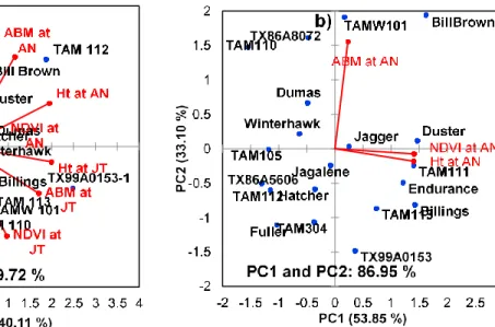
Genotype by trait biplots for trait relations and genotype comparisons…...40
Discussion……… ...44
III ASSESSMENT OF TWO GROUND-BASED CROP CANOPY SENSORS IN WINTER WHEAT……..………48
x
Introduction ……… 48
M a t e r i a l s a n d M e t h o d s … … … . 5 0 Ground based sensors……...………...53
Ground based plant health sensing system.……….………...53
Greenseeker® handheld crop sensor………..53
Field data collection………54
Aboveground biomass………...……….……...54 Plant height………...………..54 Leaf chlorophyll..………..………..….………...54 Yield………..………..54 Data analysis………...55 Results……….55
Summary statistics of field data and sensor parameters………...55
Correlation between field data and sensor parameters………....62
Evaluation of vegetation indices for the estimation of aboveground biomass and yield ………...64
Relationship between observed and predicted values of aboveground biomass and yield………68
Biplot analysis showing the performance of the twenty wheat genotypes and overall associations……….73
Discussion………...77
Genotypic variation of plant and sensor parameters across growth stages………...77
Correlation between NDVI and aboveground biomass with yield…….78
Interaction effect of genotypes, environmental conditions and years….79 Relationship between field data and sensor parameters………..79
Selection of genotypes……….80
IV NON-DESTRUCTIVE SAMPLING FOR MONITORING GROWTH, PERFORMANCE AND YIELD OF WINTER WHEAT GENOTYPES…..…82
Int roduct i on ………82
M a t e r i a l s a n d m e t h o d s … … … . 8 6 Acquisition of Aerial Imagery...………..87
Ground truth data collection ………...92
Digital photography for ground cover (GC) estimation…………....92
Aboveground biomass....………93
Yield………93
Data analysis………...93
Results………...94
Genotypic variation, growth stage and water regime………...94
Interaction among genotypes, growth stages, years and water regime……97
Correlation between SVI and field data……….99
Regression analysis……..………..103
xi
Genotypic variation and interaction between genotypes, growth
stages, years and water regime………..…111
Correlation and Regression analysis……….112
V SUMMARY AND CONCLUSION………..115
REFERENCES………...………...119
xii
LIST OF FIGURES
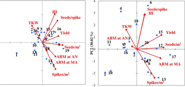
Page Figure 1 Biplot based on the twenty wheat genotypes (blue color), two water
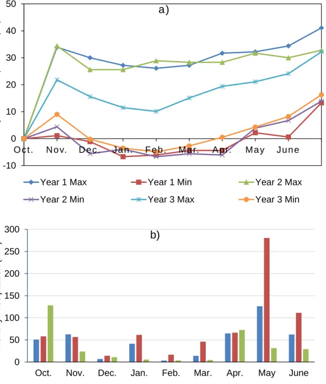
regimes (Rainfed and Irrigated) and eight traits (red color) for two years……43 Figure 2 a) Mean maximum (Max) and minimum (Min) temperatures, and b) total
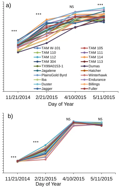
monthly precipitation from October to June for the 2012-2013 (Year 1), 2014-2015 (Year 2) and 2015-2016 (Year 3) winter wheat-growing season in Bushland, TX………..….52 Figure 3 NDVI values obtained from the Greenseeker® sensor during the growing
season in rainfed (a, c) and irrigated (b, d) fields………...…...60 Figure 4 Relationship between aboveground biomass (ABM) and NDVI at jointing
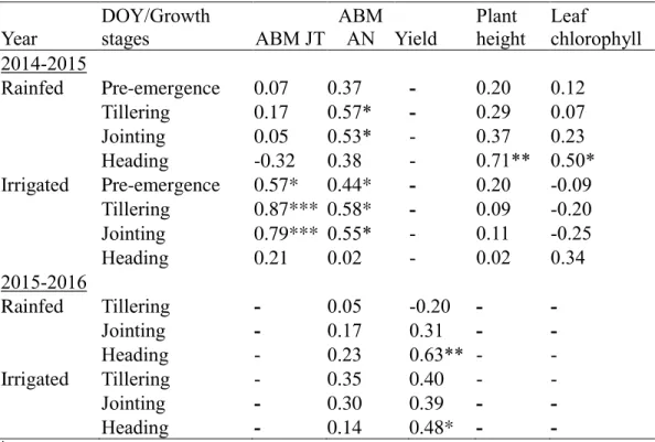
and anthesis under rainfed and irrigated fields using the NDVI values from the ground-based plant health sensing system………..…….69 Figure 5 Scatter plots showing training (black) and validation (grey) sets between
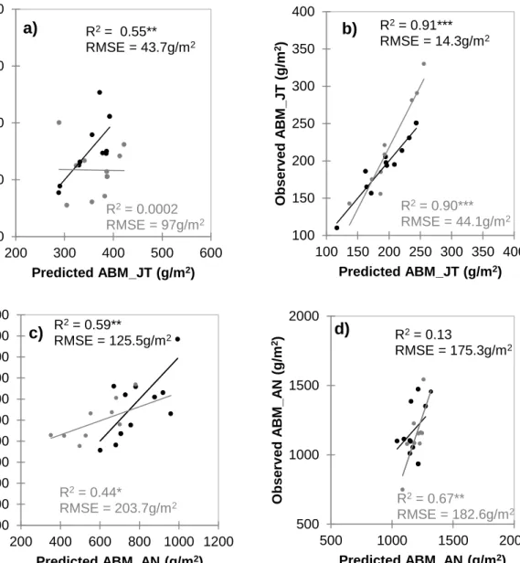
observed and predicted aboveground biomass (ABM) under rainfed (a, c) and irrigated (b, d) fields at jointing (JT) and anthesis (AN) using the NDVI values from the Greenseeker® sensor in 2014-2015 growing season (Year 2)……...71 Figure 6 Scatter plots showing training (black) and validation (grey) sets between
observed and predicted aboveground biomass (ABM), and yield under rainfed (a, c) and irrigated (b, d) fields at jointing (JT) and anthesis (AN) using the NDVI values from the Greenseeker® sensor under rainfed and irrigated fields in 2015-2016 growing season (Year 3)...72 Figure 7 Biplot showing the twenty genotypes and field parameters from the
ground-based plant health sensor under rainfed (a) and irrigated (b)
fields in year 1...75 Figure 8. Biplot showing the twenty genotypes and field parameters from the
Greenseeker® sensor under rainfed (a) and irrigated (b) fields in year 2; rainfed (c) and irrigated (d) fields in year 3………..76 Figure 9 Pictures showing the manned aircraft and the multiple camera array
Tetracam system……….89 Figure 10 Flow chart of aerial image analysis………..90 Figure 11 Aerial images of the rainfed (left) and irrigated (right) fields displayed
xiii
in color infrared………91 Figure 12 Screenshot showing the pre-processing of the digital photographs in
Adobe Photoshop……….92 Figure 13 Best Functional Relationship between field parameters and SVI for
year 1 under rainfed (a-d) and irrigated (e-h) fields………..108 Figure 14 Model Performance with percent ground cover observed and predicted for year 2………..110
xiv
LIST OF TABLES
Page Table 1 Mean maximum (Max) and minimum (Min) temperatures, and total
monthly precipitation from October to June for the 2011-2012 (Year 1)
and 2015-2016 (Year 2) winter wheat-growing season in Bushland, TX……...14 Table 2 Wheat genotypes used in this study and their pedigrees………...…………...15 Table 3 Mean sum of square for analysis of variance of 20 wheat genotypes across rainfed and irrigated environments for the growing seasons 2012-2013
(Year 1) and 2015-2016 (Year 2)………..………..19 Table 4 Mean sum of square for analysis of variance of 14 genotypes across rainfed and irrigated environments for both growing seasons………….………20 Table 5 Mean performance of aboveground biomass at anthesis and maturity, harvest index, yield and yield components for 20 genotypes across rainfed and
irrigated environments for the growing season 2012-2013 (Year 1)………..…24 Table 6 Mean performance of aboveground biomass at anthesis and harvest, harvest index, yield and yield components for 20 genotypes across rainfed and
irrigated environments for the growing season 2015-2016 (Year 2)…………..26 Table 7 Variance components and repeatability for different traits of 20 wheat
genotypes under rainfed and irrigated conditions during year 1 (a) and
year 2 (b).……….………..30 Table 8 Variance components and heritability for different traits of 20 wheat
genotypes under rainfed and irrigated conditions during year1 and year 2……32 Table 9 Phenotypic (rp) and genotypic (rg) correlation coefficient for traits in 20
wheat genotypes under rainfed and irrigated conditions during year 1…..……36 Table 10 Phenotypic (rp) and genotypic (rg) correlation coefficient for traits in 20
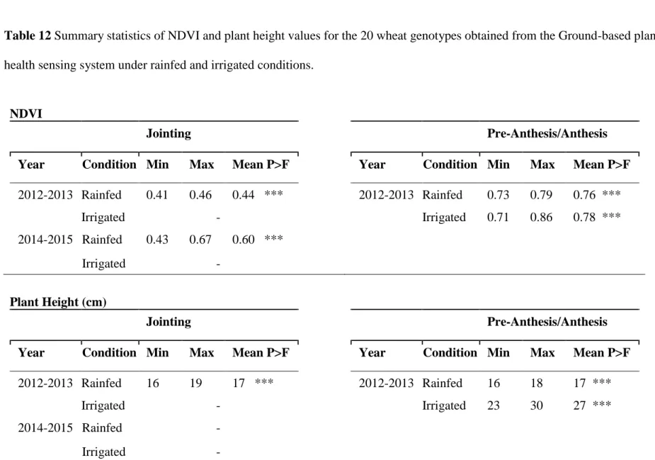
wheat genotypes under rainfed and irrigated conditions during year 2………38 Table 11 Summary statistics of plant height, leaf chlorophyll, yield, and
aboveground biomass (ABM) for the 20 genotypes……….58 Table 12 Summary statistics of NDVI and plant height values for the 20 wheat
genotypes obtained from the Ground-based plant health sensing system under rainfed and irrigated conditions………..59
xv
Table 13 Correlation between the field data and sensor parameters from the
ground-based plant health system………....63 Table 14 Correlation between the field data and the NDVI values from the
Greenseeker® sensor………...64 Table 15 The Regression models and statistics from the sensor parameters obtained from the ground-based plant health system………...66 Table 16 The Regression models and statistics from the sensor parameters obtained from the Greenseeker® sensor……….……...67 Table 17 Combined analyses of variance of the aboveground biomass (ABM) at
jointing (JT) and anthesis (AN) across three years, two water regimes
and twenty wheat genotypes………68
Table 18 Mean Maximum (Max) and Minimum (Min) temperatures, and total monthly precipitation from October to June for the 2014-2015 (Year 1) and 2015-2016 (Year 2) winter wheat-growing season in Bushland, TX…...87 Table 19 Spectral vegetation index definition………...….91 Table 20 Statistical summary of several spectral vegetation indices and field data
at three growth stages, presented for two years under rainfed and irrigated conditions……….95 Table 21 Combined analysis of variance (ANOVA) mean sum of squares for several spectral vegetation indices across three growth stages, two years and under rainfed and irrigated conditions………98 Table 22 Correlation coefficients between the spectral vegetation indices and field data...101 Table 23 Regression models and their statistics between ABM at anthesis and the spectral vegetation indices for year 1……….104 Table 24 Regression models and their statistics between ABM at jointing and the spectral vegetation indices for year 1……….105 Table 25 Regression models and their statistics between ABM at anthesis and the spectral vegetation indices for year 2……….106 Table 26 Regression models and their statistics between Yield and the spectral
1 CHAPTER I
INTRODUCTION AND LITERATURE REVIEW
Wheat (Triticum aestivum L.) is one of the world’s most important cereals and staple foods, and there is increasing demand for its production. Wheat is a major crop in the U.S. Southern Great Plains, including the Texas High Plains (Howell et al., 1995; Musick et al., 1994). The U.S. Southern Great Plains accounts for approximately 30% of total U.S. wheat production (Lollato et al., 2017). Wheat cultivation under optimum management technique requires growing the best-adapted cultivars in the most suitable environmental condition. Due to the nature of the semi-arid environment, wheat production in the area is primarily limited by drought stress during the growing season. In addition, other abiotic and biotic stresses such as heat, disease, insects, and weeds frequently hamper yield and end-use quality.
Drought is responsible for severe food shortages and famine in developing countries where irrigation facilities are not well developed to meet the transpiration needs of the crop. The Ogallala aquifer is the major water source for irrigation in the Texas High Plains. Based on the limited amount of freshwater resources available for irrigation (Botterill and Fisher, 2003), it is essential to develop production systems with limited irrigation while simultaneously improving water use efficiency. Water-use efficiency (WUE) is the amount of yield produced per unit of water lost through evapotranspiration. WUE is a physiological trait that depends on the drought tolerance of the crop defined as the ability of the plants to temporarily maintain its processes (such as photosynthesis, respiration, nutrition uptake, plant hormone functions) at low water levels. Drought tolerance is a quantitative trait with a
2
complex phenotype affected by the plant phenology. Generally, plants tend to reduce water use under drought stress. Since crop productivity is a function of water use, plant breeders are faced with the challenge of improving WUE among other traits (Blum, 2005).
Over the decades, wheat breeding has played an important role in increasing yield by developing cultivars with better drought tolerance traits. Breeding efforts for improved drought tolerance over the past few decades have revolved around the exploitation of high yield potential or selection of genotypes for morphological and physiological characters responsible for drought tolerance under various field conditions. This can be achieved partly by developing new drought-tolerant, water-efficient (Orr et al., 1998) and high yielding crop varieties. Drought tolerance is a target trait for breeding approaches to crop improvement. Over 80 years of breeding activities for major crops have led to low to moderate increase in yield under drought. Reasonable effort has been made to understand the physiological and molecular responses of plants to water deficits (Cattivelli et al., 2008). According to Nakhforoosh et al. (2016), the developments in genotyping and sequencing in the last decade have resulted in a tangible increase in genomic data. However, the genetic basis of tolerance is known to be polygenic (Ravi et al., 2011), and this brings about the major uncertainty as regards the choice of measured traits and the difficult task of ensuring an appropriate growing environment. Genotypic information must be complemented with the related plant phenotypical traits. Drought tolerance is regulated by genetic and environmental factors and by cultivation methods or crop management. To improve drought tolerance traits there is need to analyze the possible mechanisms and physiological characteristics of various wheat genotypes.
3
Wheat breeding for drought tolerance has been constrained by the absence of effective tools for the precise phenotyping of drought-related traits. The spectral reflectance methods that integrate the whole canopy for the yield assessment of many genotypes in a short time are highly desirable because field evaluation of genotypes for several years across locations is expensive and time-consuming (Reynolds et al., 1999). The advancement in remote sensing technology has recently led to the development of high-throughput phenotyping platforms (HTPPs) to overcome limitations in phenotypic data collection using conventional methods (Passioura, 2012). There is the need to implement non-destructive, easy, quick and practical tools that can evaluate large numbers of genotypes in a relatively short time. This can be done using remote sensing tools with the canopy spectral reflectance indices (SRIs) technique. This technique is based on the amount of light reflected from the canopy at a specific wavelength, due to the biochemical, physiological and structural properties of the canopy, showing spectral information to assess canopy chlorophyll content, photosynthetic efficiency, plant vigor, chlorophyll content, aboveground biomass, leaf area index, grain yield, and plant water status (Ajayi et al., 2016; El-Hendawy et al., 2015; Gutierrez et al., 2010; Prasad et al., 2007).
The crop canopy reflectance is the fraction of incoming light reflected by the crop canopy. Chlorophyll present in leaves absorbs light in the visible (VIS) light wavelengths (450-700 nanometers (nm)), with more blue (450-520 nm) and red (630-680 nm) light being absorbed than green light (520-600 nm). This results in higher reflectance in the green band, and is the reason that plants appear green to the human eyes. Compared to visible light, plants absorb much less near-infrared (NIR) light. That is, plants reflect more light in NIR wavelengths of 700-1400 nm, with percent NIR reflectance increasing as crop biomass
4
increases. The shortwave infrared wavelengths of 1400-2500 nm are characteristic of the water content in the leaves of the plant canopy. These reflectance characteristics for visible, NIR and SWIR light of crop canopies are the basis for the development of numerous vegetative indices (Araus et al., 2001).
Vegetation indices (VI) are mathematical equations of spectral bands of the electromagnetic spectrum, mainly in the VIS and NIR regions. The ratio indices were originally described by Birth and McVey (1968). Ratio indices of reflected and transmitted radiation have been used since the late 1960s to estimate plant growth. Jordan (1969) first published on the use of the simple ratio vegetation index (RVI), in which he used the ratio of transmitted radiation at 800 nm to 675 nm to estimate the leaf area index (LAI). Several band combinations have been used to define spectral vegetation indices since then, but the most common are in the strong chlorophyll absorption region (around 670 nm) and in the NIR region (750 - 900 nm), where vegetation reflects highly due to leaf cellular structure. Vegetation indices attempt to maximize the spectral contribution from green vegetation and minimize the effects of the soil background, atmosphere, and sun-target-sensor geometry. In addition, because the index is constructed as a ratio, problems of variable illumination due to topography are minimized. However, the index is susceptible to division by zero errors and the resulting measurement scale is not linear. A study regarding its efficiency has been published by Vaiopoulos et al. (2004). Since vegetation has high NIR reflectance but low red reflectance, RVI is sensitive when vegetation increases than when vegetation is low. Its sensitivity is enhanced by the Normalized Difference Vegetation Index (NDVI).
The NDVI was introduced by Rouse et al. (1974) in order to produce a spectral VI that separates green vegetation from its background soil brightness using Landsat
5
Multispectral Scanner (MSS) data. It is expressed as the difference between the NIR and red bands normalized by the sum of those bands. It is based on the contrast between the maximum absorption in the red due to chlorophyll pigments and the maximum reflection in the infrared caused by leaf cellular structure. It is the most commonly used VI as it retains the ability to minimize topographic effects while producing a linear measurement scale. In addition, division by zero errors is significantly reduced. Furthermore, the measurement scale has the desirable property of ranging from -1 to +1, with 0 representing no vegetation, negative values representing non-vegetated surfaces and positive values representing vegetation density. Light reflected from the soil can have a significant effect on NDVI values; the greater the radiance reflected from the soil, the lower the NDVI values are. NDVI is more sensitive to sparse vegetation densities and less sensitive to high vegetation densities. Other researchers have used a variation of NDVI, called green or blue NDVI (GNDVI or BNDVI), to account for variations in the green or blue band instead of a red band, which is good for estimating LAI and detecting water stress on plants (Gitelson et al., 1996; Wang et al., 2007). NDVI and RVI are the most common vegetation indices used in spectral reflectance studies today.
There exists a challenge to develop remote sensing systems that are targeted specifically to the trait of interest. Ghanem et al. (2015) noted that current HTPP systems using imaging are unable to observe plant characteristics that are targeted quantitative traits. Measurements such as plant height and leaf number, which are readily measured can indicate early plant vigor and leaf area development. These measurements seem more appropriate for the initial screening in the field. There is also an uncertainty of the choice of traits to be measured and the difficulty of ensuring an ideal and controllable experimental growing
6
environment. Morphophysiological measurements such as LAI, and the total dry weight per plant (TDW), canopy temperature (CT), leaf relative water content (RWC), leaf water potential, and water content of the aboveground biomass demonstrated strong relationships with SRIs (Barakat et al., 2016; El-Hendawy et al., 2015). The recent study showed the potential of spectral reflectance indices to detect the water status of the wheat plants and detect differences in green biomass, green leaf area, and grain yield effectively under water shortage conditions (El-Hendawy et al., 2015). The spectral reflectance indices and morphophysiological traits that are used as reliable selection criteria should have higher genetic variation and heritability (El-Hendawy et al., 2015). El-Hendawy et al. (2017) considered the performance of wheat genotypes under different water regimes and tested the relationships between SRIs and drought tolerance indices with grain yield. Their results show that selection based on the drought tolerance indices has the possibility to identify wheat genotypes that produce desirable yields in both normal and stress conditions. The use of either vegetation or water SRI to predict grain yield is also dependent on the phenological growth stage. The response of the plant due to water stress can be observed in the production of photo assimilates, and their further transformation into grain yield.
Infrared thermography involves low-cost CT measurements for high-throughput field phenotyping. The CT is an indicator of crop water stress. Canopy temperature depression (CTD) is the difference between air temperature and CT; it gives indirect estimate of stomatal conductance, leaf chlorophyll, leaf water potential and grain yield. A cooler canopy (higher CTD) may be one of the reasons for higher wheat yield under dryland conditions (Pradhan et al., 2014). Bellundagi et al. (2013) supported their findings with additional field data such as ground cover, flag leaf area, and leaf relative water content.
7
Another approach is the use of thermal infrared (TIR) detectors to measure plant temperature which may vary due to partial stomatal closure. That is, the soil water being conserved by the plant may be due to partial stomatal closure under high atmospheric vapor pressure deficit, leading to yield increase. TIR can be useful also as an early indirect selection to eliminate those lines that under high vapor pressure deficit conditions exhibit low temperatures (Ghanem et al., 2015). Wheat breeders can improve on these characteristics which may have a significant effect on grain yield.
Overall, the factors to be considered for water use efficiency and drought tolerance are those that are responsible for wheat cultivars to perform optimally under drought stress. These include i) ability to capture more soil water; ii) ability to optimize the available water for efficient use; and iii) partitioning assimilates for reproductive growth under stress (Aparicio et al., 2002b; Lorens et al., 1987; Reynolds et al., 2005). All these can be monitored and assessed throughout the growing season and under water-stressed condition using remote sensing tools as indirect selection criteria for drought tolerance and water use efficiency. The progress of wheat breeding requires accurate physiological phenotyping of the desirable traits. However, it is difficult and complex to phenotype for traits that are not visible to the naked eyes. A well-planned step by step physiological phenotyping approach will assist to effectively address the challenge of integrating phenotyping in a breeding program. For improved breeding and phenotyping effort in identifying drought tolerance and water use efficient genotypes, the following steps can be noted. This include: i) selecting traits that are evidently going to improve the crop productivity; ii) having basic knowledge of the trait to direct the indirect selection approach; and iii) developing several phenotypic and genotypic screening for insight on the trait expression at various growth stages (also
8
across years and location) in the breeding process (Ghanem et al., 2015; Glazier et al., 2002; Miflin, 2000).
This dissertation focuses on the evaluation of aboveground biomass, yield and its components, assessment of remote sensors both ground-based and aerial systems, under rainfed and irrigated conditions. Chapter II covers the evaluation of wheat genotypes for their yield potential and dry matter accumulation and their relation to yield component traits to identify sources of germplasm for breeding drought tolerance. Chapter III, IV, and V reflect on the use of ground-based and aerial remote sensors to assess the growth, performance and yield of winter wheat genotypes. Development of stress tolerant cultivars is always a major objective of many breeding programs. However, success has been limited by inadequate screening techniques in identifying genotypes that show clear differences in response to various environmental stresses during the growing season. The overall objective of this study was to develop and evaluate remote sensing techniques for assessing phenotypic traits of winter wheat genotypes in the Texas High Plains.
9 CHAPTER II
GENETIC VARIABILITY AND TRAIT ASSOCIATION WITH YIELD IN WINTER WHEAT (Triticum aestivum L.) UNDER IRRIGATED AND RAINFED
CONDITIONS INTRODUCTION
In most wheat (Triticum aestivum L.) breeding programs, yield is the major selection criterion influenced directly and indirectly by several environmental, morphological, physiological, biochemical, and metabolic plant processes, where their genetics and relationships are unclearly known (Jackson et al., 1996; Orr et al., 1998). Yield is a quantitative trait that may be influenced by the following morpho-physiological and yield component traits: canopy temperature (CT), leaf relative water content, leaf water
potential, water content of the aboveground biomass, photosynthetic efficiency, plant vigor, chlorophyll content, leaf area index, plant height, harvest index (HI), number of spikes/m2, seeds/spike, and 1000-kernel weight (TKW). Wheat yields are reduced when the plant is water-stressed as a result of the physiological and biochemical processes being altered (Lascano et al., 2001). Hence, the life cycle of the plant is shortened by reducing the size of organs such as leaves, tillers, spikes, the number of spikelets, and the ratio of spike dry weight to total dry weight. Yield components are determined throughout the development and growth during wheat growing season. The three yield components include spikes per unit area, seeds per spike and seed weight. The product of these components is yield, when measured without error and expressed in the appropriate unit. The development of high-yielding genotypes through identifying drought tolerant mechanisms is important for increasing yield potential under both rainfed and irrigated conditions. The quantitative variation in a plant population is based on the phenotypic,
10
genotypic and environmental variation. The phenotypic variance includes genetic variance, genotype x environment interaction and error variance (Acquaah, 2012). Wheat breeders improve large populations by selecting genotypes based on their phenotypes. The genetic component of variation is important as a result of being transferred to the next generation (Hamdi, 1992). Genetic variability among wheat genotypes can be estimated based on qualitative and quantitative traits. Heritability in broad sense, it is the ratio of genotypic variation to the phenotypic variance, which is the proportion of phenotypic variance due to solely genetic differences i.e. heritable. Heritability varies from zero to one; from no genetic contribution (instead all environment) to all genetic contribution, respectively (Acquaah, 2012).
Yield selection under drought stress conditions is difficult as a result of its low heritability due to variations in the magnitude of the stress conditions on the field (Ludlow and Muchow, 1990; Yağdi and Sozen, 2009). In all studies that are dedicated to drought tolerance the crucial aspect is the assessment of the degree of drought tolerance in different genotypes. In many studies the identification of tolerant and susceptible genotypes is based on few plant traits related to drought response such as stomatal conductance,
photosynthetic capacity, rooting depth, osmotic adjustment (Araus et al., 2002; Cattivelli et al., 2008). Selection for drought tolerant wheat genotypes may be more efficient under well-watered conditions than under water-stressed conditions, with identifying genotypes with higher yield potential than others (Rajaram, 2001; Rajaram et al., 1996). Grain yield selection is a conventional approach when measuring yield itself, whereas it is a logical approach when considering indirect traits (Richards, 1996). Kashif and Khaliq (2004) suggested that indirect selection for yield using its components, might be more effective
11
than direct selection. This is because of low heritability for yield, also when the component has a higher heritability than yield and the genetic correlation between the two traits is high. The difficulty in identifying a physiological parameter as a reliable indicator of yield in dry conditions has suggested that yield performance over a range of environments should be used as the main indicator for drought tolerance (Voltas et al., 2005). The selection for drought tolerant genotypes should be based on important
morpho-physiological and yield component traits, not only on yield. In order to make good use of the genetic variability among the large population, there is need to have information about the mutual association between yield and yield components. That is, the correlation coefficients of various component traits with yield and among themselves (Mary and Gopalan, 2006).
The ability to discriminate among performance of different genotypes depends on the information on the environment (E) where the plant are growing so as to separate genotypic effects (G) from the total phenotype (P) where (P=G+E+G*E). Also one can evaluate and relate the response of similar genotypes in different environment or vice-versa (Orr et al., 1998). The genotype by environment interaction (G*E or GEI) is the interaction of genotype with the factors (either environmental or physiological) that can affect the expression of a trait. According to Reynolds et al. (2001), traits which have less G*E have their genotypes classified based on these traits and despite their trait expression, will mostly maintain their classification across different environments. These traits are highly heritable with limited environmental effect on their expression, hence these traits will be effectively selected across locations and years. Generally, there is a greater probability of
12
obtaining significant G*E when the genetic complexity of a trait is greater (Alberts, 2004; Reynolds et al., 2001).
The size of genetic variability in a population and the extent of heritability of the desirable traits, determine the rate of genetic gain for yield in a breeding program. The objective of this study was to investigate plant traits that contribute to yield under different two water regimes – rainfed and irrigated, and to what extent these traits may be
considered as specific selection criteria for tolerance to drought stress conditions in the Southern Great Plains (SGP). These objectives was achieved by estimating genetic
variability, identifying traits that impact drought tolerance, estimate the extent of genotypic and phenotypic variability (heritability) and evaluate association among the yield and yield components among the 20 wheat genotypes.
MATERIALS AND METHODS Description of Study Area
Field experiment was conducted at the Texas A&M AgriLife Research Experiment Station, Bushland, Texas (Lat. 35º11’N, Long. 102º06’W; elevation 1170m above the mean sea level) during the 2011-2012 (Year 1) and 2015-2016 (Year 2) growing seasons. The soil type was Pullman clay loam (fine, mixed, thermic Torrertic Paleustoll: USDA classification) described by Unger and Pringle (1981). The climatic condition was semi-arid with erratic precipitation and high evaporative demands. Weather data (Table 1) was downloaded for the Bushland station for Year 1 and Year 2 from the Texas High Plains Evapotranspiration (TXHPET) Network (http://txhighplainset.tamu.edu) and US Climate Data Network (http://usclimatedata.com), respectively. Precipitation was significantly and generally lower for year 1 than year 2, especially at the earlier and later growth stages, that is pre-emergence
13
and anthesis, respectively. The total precipitation during the growing season was 166 mm and 310 mm (Year 1 and 2), and the average maximum and minimum temperature during the growing season was 18.4 ºC and 1.8 ºC, respectively, in 2011-2012, and 21.6 ºC and 4.5 ºC, respectively, in 2015-2016. Although the temperature in year 2 was generally higher, it can be explained by the increased precipitation. Overall, year 1 had wheat plants more water stressed throughout the entire growing season.
Experimental Design
Twenty winter wheat genotypes were grown under two water regimes – rainfed and irrigated, during 2011-2012 and 2015-2016. Ten of these genotypes were developed by the Texas A&M wheat breeding program, while the other ten were developed by wheat
breeding programs from Kansas, Colorado, Oklahoma and Nebraska. As seen in Table 2, these genotypes consist of wide genetic background based on their pedigree. In the irrigated treatment, irrigation was applied several times during the wheat growing season to supplement seasonal rainfall. The experimental design was a randomized complete block design (RCBD) with three replications. The seeding rate for irrigated and rainfed fields, was 100 kg/ha and 67 kg/ha, respectively. The plot size for irrigated plots was 1.52 m x 3.05m (4.64 m2) and 1.52 m x 4.27 m (7.0 m2) for rainfed plots, while the row spacing for all plots was 18 cm.
14
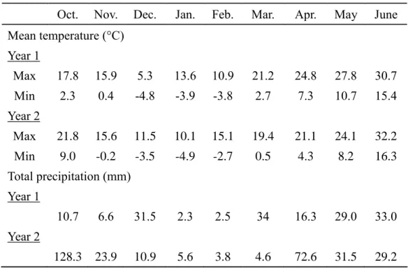
Table 1 Mean maximum (Max) and minimum (Min) temperatures, and total monthly precipitation from October to June for the 2011-2012 (Year 1) and 2015-2016 (Year 2) in Bushland, TX.
Oct. Nov. Dec. Jan. Feb. Mar. Apr. May June Mean temperature (°C) Year 1 Max 17.8 15.9 5.3 13.6 10.9 21.2 24.8 27.8 30.7 Min 2.3 0.4 -4.8 -3.9 -3.8 2.7 7.3 10.7 15.4 Year 2 Max 21.8 15.6 11.5 10.1 15.1 19.4 21.1 24.1 32.2 Min 9.0 -0.2 -3.5 -4.9 -2.7 0.5 4.3 8.2 16.3 Total precipitation (mm) Year 1 10.7 6.6 31.5 2.3 2.5 34 16.3 29.0 33.0 Year 2 128.3 23.9 10.9 5.6 3.8 4.6 72.6 31.5 29.2
15
Table 2 Wheat genotypes used in this study and their pedigrees.
Name
Year of
release Pedigree
TAM W-101 1971 KS56761/Bison (=TX65A1682) (CI 15324) TAM 105 1979 Short wheat/Sturdy composite bulk selection TAM 110† 1996 TXGH12588-105=(TAM 105*4/Amigo*4//Largo) TAM 111 2003 TAM 107/TX78V3620/CTK78/3/TX87V1233 TAM 112† 2005 105*4/Amigo*4//Largo)
TAM 304 2007 TX01D3232=TX92U3060/TX91D6564 (=X95U104-P66)
TAM 113 2010 TX02A0252=TX90V6313//TX94V3724(TAM-200 BC41254-1-8-1-1/TX86V1405
TX99A0153-1† Not released Ogallala/TAM-202
TX86A5606† Not released TAM 105*4/ Amigo*4//Largo TX86A8072† Not released TAM 105*4/ Amigo*4//Largo TAM 114 2014
TX07A001505=T107//TX98V3620/Ctk78/3/TX87V1233/4/N87V106//TX 86V1540/T200
TX11Vsyn0101 Not released TAM 111*2/CIMMYT E95Syn4152-5 PlainsGoldByrd Not released CO06424=TAM 112/CO970547-7
Iba 2013 OK07209=OK93P656-(RMH 3299)/OK99621 F4:10 AMPSY068 Not released TAM 111*2/CIMMYT E951yn4152-37
AMPSY588 Not released TAM 112/CIMMYT E951yn4152-46//TAM 112 Dumas 2000 WI90-425/WI89-483 Jagalene 2001 Abilene/Jagger Hatcher 2005 Yumar/PI372129//TAM-200/3/4*Yumar/4/KS91H184/Vista BillBrown 2007 Yumar/Arlin Winterhawk 2007 474S10-1/X87897-26//HBK0736-3 Endurance 2004 HBY756A/´Siouxland`//´2180` Duster 2006 OK93P656H3299-2C04=WO405D/HGF112//W7469C/HCF012 Billings 2009 OK03522=N566/OK94P597 F4:14
Jagger 1994 KS82W418/Stephens (=KS84063-9-39-3) (PI 593688) Fuller 2006 KS00F5-14-7=BULK SELN
†The genotype has 1AL.1RS rye translocation.
Data collection
Aboveground biomass was collected at anthesis and at maturity; 50 cm of one row was cut at ground level from each plot. For each sample, the stems (including leaves and leaf sheaths) and heads were separated and counted. To determine the dry biomass, the stems and heads were dried at 60°C for 72 hours.
16
Yields were obtained by machine-harvesting with a Wintersteiger plot combine. The yield based on about 10 % moisture content was expressed on a kilogram per hectare basis. To calculate the harvest index (grain yield divided by aboveground biomass), grain yield or seed weight was obtained from 50 cm of one row at maturity. The four yield
components (spikes per square meter, seeds per spike, thousand-kernel weight (TKW), and seeds per square meter) were determined. The threshed seeds were weighed after dried to 0% moisture at 130°C for 19 h (ASAE, 1998). Then, the TKW was calculated by weighing 250 seeds and multiplied by four. Seeds per spike and seeds per square meter were
determined by dividing the total number of seeds by the number of spikes per sample and then dividing by sample area.
Data Analysis
Statistical analysis carried out in this study was done using the SAS version 9.3 (Statistical Analysis System Institute, Cary, NC, USA), META-R (Multi Environment Trial Analysis with R) macro (Alvarado et al., 2015) and XLSTAT developed by Addinsoft (2010) for Microsoft Excel. Analysis of variance (ANOVA) was performed using the General Linear Model procedure. Individual water regime data were subjected to ANOVA to determine the significance of genotypic component in each environment. Analysis of variance was performed using the following equation to determine if there was a significant effect of genotype, year, and environment, genotype x environment, and genotype x year interactions on the traits:
17
where Yijkl is the measurement of genotype k on plot l in block j, and environment i; μ is
the overall mean of all plots in all environments; Ei is the effect of environment i; Bji is the
effect of block j within environment i using replication; Gk is the effect of genotype k; GEik
is the interaction of genotype i with experiment k;
ε
ijkl is the plot residual.Means of the individual environment data was subjected to ANOVA to determine the significance of genotypic component in each environment. Significant means were
compared using least significant difference (LSD) multiple means comparison technique at Probability value ≤ 0.05. The statistical model used for individual environment analysis was as follows:
Yik= μ + Rk + Gi + Ɛik
Where Yik is the observed phenotypic value of the ith genotype in kth replicate, μ is the overall mean, Rk is the replication effect, Gi is the genetic effect of ith genotype and Ɛik is
the residual.
Using the META-R, heritability in a broad sense was estimated from the result of variance analysis according to the formula used by Burton and Devane (1953), also computing phenotypic and environmental variance. Genotypic and phenotypic correlations were worked out according to the method given by Burton (1952) and Kwon and Torrie (1964). Phenotypic (δ2p) and genotypic (δ2g) variances were obtained according to Baye
(2002) as δ2g = MSp –(MSe/r), and δ2p = MSg/r, where MSp and MSgare mean squares of
phenotypes and genotypes, respectively; r was number of replication. The mean values were used for genetic analyses to determine phenotypic coefficient of variation (PCV) and
18
genotypic coefficient of variation (GCV) using the variances (δ2) and mean (x), according
to Singh and Chaudhary (1979) as:
GCV (%) = √(δ2g)/x * 100 PCV (%) = √(δ2p)/x * 100
Broad-sense heritability (h2) or repeatability estimate of each trait was computed as: Heritability (h2) = δ2g/ δ2p
Principal component analysis for GGE (i.e., G = genotype and GE = genotype by environment and/or trait interaction) was performed to visualize relationships among genotypes and environment and/or traits by using the genotypic means of each environment in the XLSTAT software.
RESULTS
Analysis of variance and mean performance
The analysis of variance indicated the existence of highly significant variability for all the traits studied (Table 3). For year 1, the mean sum of squares due to genotype x environment interaction was high for only spikes/m2, TKW, and yield. There was no genotype x environment interaction for year 2. Environmental (water regime) variance for all traits appeared significant for both years, except spikes/m2 and seeds per spikefor year 2. For year 1, the mean sum of squares due to genotypes was high for all the traits except aboveground biomass at anthesis. Year 2 recorded all traits with high mean sum of squares due to genotypes except aboveground biomass at maturity and anthesis.
19
Table 3 Mean sum of square for analysis of variance of 20 wheat genotypes across rainfed and irrigated environments for the growing seasons 2011-2012 (Year 1) and 2015-2016 (Year 2).
Traits Genotype (G) Environment (E) G x E
Year 1 Biomass at MA 50861.64* 31549138.32*** 31285.21 Harvest index 0.006** 0.06*** 0.002 Spikes/m2 48797.71* 13035001.06*** 46060.61* Seeds/spike 25.42** 32.12* 9.37 Seeds/m2 19322982** 3944076122*** 9042614 Biomass at AN 28727.22 12607509.58*** 23290.52 Yield 9283.99** 3620502.06*** 8394.99*** TKW 19.43* 1488.54*** 16.55* Year 2 Biomass at MA 66460.37 932489.49** 116657.21 Harvest index 0.005* 0.13*** 0.003 Spikes/m2 113719.81*** 51405.25 53892.04 Seeds/spike 23.35*** 6.62 4.54 Seeds/m2 32338913.1** 279129908*** 18565758 Biomass at AN 48101.65 5500586.74*** 49470.53 Yield 6009.93* 1069523.69*** 3687.49 TKW 38.22*** 263.70*** 3.03
*, **, and ***Significant at0.05, 0.01 and <.0001, respectively
Similar genotypes (14 total) that were planted in both year 1 and 2 were selected to perform analysis of variance for year and genotype x year interaction (Table 4). Significant interaction exists among the 14 genotypes and years only with spikes/m2, seeds per spike
and TKW. The year effect was highly significant for all the traits, so also the genotypes for all traits except seeds/m2, aboveground biomass at maturity and anthesis.
20
Table 4 Mean sum of square for analysis of variance of 14 genotypes across rainfed and irrigated environments for both growing seasons.
Source Genotype (G) Year (Y) G x Y
Trait/df 13 3 39 Biomass at MA 78929.29 13200034.99*** 67169.98 Harvest index 0.005* 0.07*** 0.003 Spikes/m2 109525.62*** 3602351.25*** 59236.19** Seeds/spike 23.41*** 77.62*** 9.36* Seeds/m2 23726362 1061609004*** 14305562 Biomass at AN 21305.37 4300849.08*** 37862.08 Yield 11278.48** 1372253.89*** 5959.45 TKW 32.08*** 1820.77*** 8.28*
*, **, and ***Significant at0.05, 0.01 and <.0001, respectively
There was considerable variability in the mean values of aboveground biomass, yield and yield component traits in each individual environment for each of the two years (Tables 5 and 6). Significant variation was found among the 20 genotypes for only TKW for year 1 under rainfed condition. Under irrigated condition, all traits were significantly different among the 20 wheat genotypes except aboveground biomass, harvest, and TKW. The study in Year 2 under rainfed condition showed significant differences in spikes/m2 and TKW among the 20 wheat genotypes. Under irrigated condition, all traits appeared significantly different among the genotypes except aboveground biomass at anthesis and maturity.
According to the means of three replications for year 1 (Table 5), the aboveground biomass at maturity was between 364 and 592 g/m2 (average of 458 g/m2) and, 1241 and 1787 g/m2 (average of 1484 g/m2) under rainfed and irrigated conditions, respectively.
21
Jagger was the highest followed by TX99A0153-1, Billings, Winterhawk, Endurance, TAM 111, Hatcher, TAM 112, and TAM 113 under rainfed condition in year 1. Under irrigated condition for year 1, Hatcher had the highest aboveground biomass at maturity, followed by Winterhawk, Duster, TX99A0153-1, and TAM 113, while the lowest was found with TAM 110, and Dumas. For year 2 (Table 6), the aboveground biomass at maturity was determined between 1178 and 2000 g/m2 (average of 1519 g/m2) and, 1434
and 2020 g/m2 (average of 1696 g/m2) under rainfed and irrigated conditions, respectively. Under rainfed condition, TAM 105 had the highest aboveground biomass at maturity, the lowest was TX99A0153-1, and Iba, while TAM 304 had the highest under irrigated condition and the lowest was Dumas and TAM 110. Aboveground biomass at anthesis for year 1 under rainfed condition ranged from 345 to 583 g/m2 with TAM 113 and
TX99A0153-1 as the minimum and maximum, respectively. Values under irrigated condition ranged from 887 to 1261 g/m2 with TAM 110 and Jagger as the minimum and
maximum, respectively.
Harvest index values were generally within 0.18 and 0.38 under rainfed condition and within 0.27 and 0.41 under irrigated condition for both years. Endurance (0.38), TAM 110, TX99A0153-1, TX86A5606 and Duster (0.36), and Jagalene (0.35) had the highest harvest index value under rainfed condition for year 1, while year 2 recorded TAM 112 (0.33), TAM 111 and Winterhawk (0.31), TAM 105 (0.29), TAM 113 (0.28), TAM 304 and Hatcher (0.27) as the highest. Lowest under year 1 was TAM W-101 (0.22), and under year 2 was TX11Vsyn0101 and TAM 114 (0.18), and TX99A0153-1 (0.19).
TAM 112 (652) and BillBrown (529) had the highest spikes/m2, the lowest was Fuller (334) and TAM 105 (337) under rainfed condition in year 1. Year 2 had TAM 105
22
(1537) has the significantly highest spikes/m2 value and TX99A0153-1 (731) as the
significantly lowest value. Under irrigated condition in year 1, the value was between 772 and 1339 with TAM 111 and Duster as the minimum and maximum, respectively.
Spikes/m2 in year 2 under irrigated condition ranged from 709 to 1244, with AMPSY 068 and Iba as the significantly lowest and highest, respectively.
For year 1, seeds per spike values ranged from approximately 10 to 20 with TAM W-101 and Endurance as the minimum and maximum, respectively under rainfed
condition. Seeds per spike values ranged from 12 to 24 under irrigated condition, with TAM W-101 and TAM 304 as the minimum and maximum, respectively. Seeds/m2 values were between 3800 and 10538 for TAM W-101 and Jagger respectively, under rainfed condition, while under irrigated condition the values were significantly higher and was between 13133 and 24020 for TAM W-101 and Duster respectively, for year 1. Year 2 under rainfed condition had seeds/m2 values ranged from 6926 and 19451 for
TX99A0153-1 and TAM 105, respectively. Under irrigated condition, seeds/m2 values were between 12131 and 20956 for Hatcher and TAM 304, respectively.
Thousand-kernel weight (TKW) ranged from 14 g to 26 g under rainfed condition in year 1 with BillBrown and TAM W-101 as the lowest and highest, respectively and year 2 it ranged from 27 to 40 g with Duster and AMPSY 068 as the minimum and maximum, respectively. For year 1 under irrigated condition, TKW ranged from 24 g in BillBrown to 33 g in Billings. In year 2, TKW ranged from 31 to 40 g with Plains Gold Byrd, TAM 105, and Duster as the lowest (31 g) and AMPSY 068 and Billings as the highest
23
Yield values under rainfed condition for year 1 was determined between 66 and 105 g/m2 with TAM W-101 and TAM 112 as the minimum and maximum, respectively. Year 2 was found between 249 and 411 g/m2 with TAM 114 and Plains Gold Byrd as lowest and highest, respectively. Irrigated condition for year 1 recorded yield values that ranged from 414 to 649 g/m2 with TAM W-101 and Winterhawk as the minimum and maximum, respectively. Yield values for year 2 was between 433 and 549 g/m2 with TAM 105 and
Plains Gold Byrd as the minimum and maximum, respectively. Generally, TAM genotypes showed more similar values for yield, and yield component traits compared to the other genotypes.
24
Table 5 Mean performance of aboveground biomass at anthesis and maturity, harvest index, yield and yield components for 20 genotypes across rainfed and irrigated environments for the growing season 2011-2012 (Year 1).
Genotype Biomass at MA HI Spikes Seeds/ spike Seeds Biomass at AN Yield TKW g/m2 no./m2 no./m2 g/m2 g/m2 g Rainfed TAM W-101 439.93 0.22 401.20 9.63 3800.38 415.67 66.23 26.20 TAM 105 364.42 0.30 337.46 16.69 5392.12 470.87 86.16 23.10 TAM 110 388.11 0.36 412.45 17.12 7021.69 359.77 86.47 19.90 TAM 111 477.05 0.32 397.45 16.18 6415.67 454.22 87.59 23.40 TAM 112 474.43 0.28 652.42 13.00 7651.11 483.16 104.97 17.80 TAM 304 429.77 0.31 431.20 17.67 7787.49 377.02 78.50 17.10 TAM 113 472.97 0.29 419.95 14.22 6200.27 344.73 99.76 22.70 TX99A0153-1 531.23 0.36 487.44 17.34 8641.72 582.86 103.95 21.90 TX86A5606 386.99 0.36 408.70 16.32 6689.52 351.74 83.51 21.40 TX86A8072 436.22 0.30 419.95 14.64 6146.94 425.42 78.91 21.60 Dumas 460.55 0.26 442.44 14.29 6310.28 461.12 77.48 19.40 Jagalene 457.93 0.35 464.94 16.01 7421.64 428.20 99.96 21.80 Hatcher 476.12 0.24 408.70 14.31 5843.65 400.34 86.16 20.00 BillBrown 448.52 0.26 528.68 16.10 8491.31 461.98 78.09 14.30 Winterhawk 500.79 0.34 386.20 17.66 6812.25 447.99 98.02 24.90 Endurance 482.41 0.38 457.44 19.66 8955.62 383.31 100.17 20.40 Duster 447.54 0.36 438.70 17.78 7732.76 461.57 96.79 20.60 Billings 518.82 0.30 468.69 14.94 6935.65 395.58 95.87 21.80 Jagger 592.05 0.32 536.18 19.48 10538.4 414.96 101.19 18.20 Fuller 377.88 0.31 333.71 16.63 5644.35 483.05 90.97 20.70 Mean 458.19 0.31 441.69 15.98 7021.64 430.18 90.04 19.57 LSD (0.05) NS NS NS NS NS NS NS 3.09
25 Table 5 Continued. Genotype Biomass at MA HI Spikes Seeds/ spike Seeds Biomass at AN Yield TKW g/m2 no./m2 no./m2 g/m2 g/m2 g Irrigated TAM W-101 1311.06 0.31 1106.11 12.16 13132.75 986.43 413.65 31.50 TAM 105 1394.38 0.36 1106.11 16.68 18407.90 918.15 500.15 27.20 TAM 110 1241.21 0.39 1102.36 15.30 16861.66 886.73 478.85 28.40 TAM 111 1319.16 0.39 772.40 21.62 16471.74 1182.26 514.32 31.40 TAM 112 1425.95 0.37 1053.62 16.48 16973.35 1032.25 527.71 31.10 TAM 304 1481.59 0.41 869.89 23.97 20731.84 1117.36 603.49 29.10 TAM 113 1609.67 0.32 1267.34 16.17 20451.06 1108.44 526.13 25.40 TX99A0153-1 1631.50 0.34 1248.59 15.45 19389.51 1068.47 561.94 29.20 TX86A5606 1309.86 0.37 1064.87 15.68 16348.40 964.57 488.64 29.50 TX86A8072 1391.86 0.30 1031.12 14.20 14686.87 1308.06 419.65 28.30 Dumas 1269.48 0.34 847.39 17.60 15085.48 1155.42 425.50 28.40 Jagalene 1512.56 0.39 1267.34 17.20 21900.27 910.16 582.49 26.80 Hatcher 1787.74 0.32 1421.07 14.74 20713.59 992.31 571.62 28.00 BillBrown 1527.37 0.35 1109.86 16.63 18814.31 1116.54 532.77 24.40 Winterhawk 1723.02 0.38 1154.86 17.95 20503.62 1125.35 649.08 31.70 Endurance 1412.19 0.35 1042.37 16.43 17144.61 1168.84 489.39 28.80 Duster 1686.28 0.37 1338.58 17.81 24020.27 1000.30 622.31 25.90 Billings 1517.89 0.39 963.63 18.45 17732.25 1038.06 583.76 32.90 Jagger 1529.62 0.34 1181.10 17.70 20812.02 1261.15 524.63 25.70 Fuller 1591.26 0.35 1068.62 18.14 19571.36 1228.08 556.28 28.60 Mean 1483.68 0.36 1100.86 17.02 18487.64 1078.45 437.43 26.61 LSD (0.05) NS NS 309.89 3.56 5744.90 NS 151.72 NS
26
Table 6 Mean performance of aboveground biomass at anthesis and harvest, harvest index, yield and yield components for 20 genotypes across rainfed and irrigated environments for the growing season 2015-2016 (Year 2).
Genotype Biomass at MA HI Spikes Seeds/ spike Seeds Biomass at AN Yield TKW g/m2 no./m2 no./m2 g/m2 g/m2 g Rainfed TAM 105 1999.70 0.29 1537.31 20.26 19451.35 654.26 368.49 29.23 TAM 110 1603.67 0.23 1199.85 16.44 11578.89 796.36 354.74 31.77 TAM 111 1529.36 0.31 854.89 19.97 13919.13 636.90 366.65 34.03 TAM 112 1695.46 0.33 1057.37 20.30 16785.42 612.37 329.21 33.10 TAM 113 1788.75 0.28 967.38 19.84 16269.75 662.43 362.21 32.20 TAM 114 1470.30 0.18 1023.62 18.16 10190.72 839.56 249.43 29.07 TAM 304 1479.30 0.27 952.38 20.05 13697.45 904.65 287.94 29.57 TX99A0153-1 1177.95 0.19 731.16 13.84 6926.44 729.17 288.48 33.45 Dumas 1367.90 0.22 806.15 18.02 9822.90 739.82 286.35 29.77 Jagalene 1439.33 0.29 926.13 21.00 12896.25 928.23 303.01 31.80 Hatcher 1463.74 0.27 971.13 18.81 11845.94 895.09 330.40 32.90 Plains Gold Byrd 1541.92 0.30 1012.37 21.45 15757.93 811.47 411.30 30.27 Winterhawk 1483.50 0.31 1117.36 19.92 14690.38 840.76 332.39 33.50 Iba 1237.50 0.25 1072.37 22.19 11267.26 785.30 379.58 28.73 Endurance 1531.55 0.23 933.63 19.69 13079.25 547.96 274.22 31.30 Duster 1537.53 0.25 1154.86 22.73 14821.31 629.32 334.77 27.23 Billings 1514.29 0.22 858.64 15.43 10102.05 528.20 271.42 33.50 AMPSY068 1369.78 0.24 693.66 15.61 8701.52 708.17 296.53 39.83 AMPSY588 1414.74 0.22 914.89 15.76 9681.18 776.98 293.08 35.80 TX11Vsyn0101 1546.74 0.18 849.27 14.25 9532.63 697.23 238.49 32.60 Mean 1518.44 0.26 986.28 18.84 12654.25 736.21 317.93 31.96 LSD (0.05) NS NS NS 4.54 NS NS NS 2.03
27 Table 6 Continued. Genotype Biomass at MA HI Spikes Seeds/ spike Seeds Biomass at AN Yield TKW g/m2 no./m2 no./m2 g/m2 g/m2 g Irrigated TAM 105 1505.77 0.27 941.13 17.78 12633.32 1108.85 433.03 31.67 TAM 110 1454.22 0.35 1038.62 19.72 14110.98 1013.21 462.68 35.67 TAM 111 1653.43 0.36 824.90 19.99 16371.41 1119.46 519.67 36.33 TAM 112 1773.30 0.35 997.38 19.23 17372.83 1136.86 509.35 36.33 TAM 113 1675.70 0.32 933.63 19.00 15226.37 1204.31 533.87 35.33 TAM 114 1630.75 0.29 978.63 19.68 13972.60 1456.51 494.97 33.67 TAM 304 2019.72 0.34 1031.12 21.51 20956.15 1258.33 528.99 32.33 TX99A0153-1 1885.86 0.28 1113.61 16.03 14980.30 1037.83 521.79 35.00 Dumas 1434.27 0.31 727.41 19.92 13746.17 1000.75 447.69 33.00 Jagalene 1714.85 0.33 937.38 18.92 15909.51 951.46 460.78 36.00 Hatcher 1553.54 0.28 869.89 17.95 12131.09 1240.45 535.48 36.33 Plains Gold Byrd 1943.61 0.33 1214.85 21.94 20874.93 1329.86 548.53 31.00 Winterhawk 1506.26 0.32 787.40 18.37 13437.51 1255.98 531.29 35.67 Iba 1998.16 0.33 1244.84 21.72 20061.33 1221.04 547.92 33.33 Endurance 1724.18 0.35 907.39 20.63 17341.74 1232.62 498.88 34.67 Duster 1846.08 0.32 1094.86 21.35 18446.79 1083.28 535.34 31.33 Billings 1814.59 0.32 802.40 16.50 15007.70 1418.67 513.65 39.00 AMPSY068 1539.18 0.33 708.66 16.88 12761.07 1369.33 512.40 39.67 AMPSY588 1646.53 0.33 963.63 18.11 14979.28 1136.03 504.58 37.00 TX11Vsyn0101 1602.29 0.29 731.16 18.08 12625.06 966.82 494.08 37.00 Mean 1696.12 0.32 942.45 19.17 15647.31 1179.33 506.75 35.02 LSD (0.05) NS 0.05 229.28 1.66 4046.60 NS 59.18 2.64
28
Variances, coefficient of variability and heritability for traits in the 20 wheat genotypes
The estimates of phenotypic variance, genotypic variance, environmental variance, broad sense heritability or repeatability, phenotypic and genotypic coefficient of variability (PCV and GCV) for year 1 and 2 are given in Tables 7 and 8. Generally, it was observed that the phenotypic variance was significantly greater than the genotypic and
environmental variances for all traits under both water regimes and years. The
environmental variance was greater than the genotypic variance for all the traits under both water regimes and years, with some exceptions such as; aboveground biomass at maturity under irrigated condition for year 1, seeds/spike and TKW under rainfed condition for year 2, spikes/m2, seeds/spike, seeds/m2, and TKW under irrigated condition for year 2. As seen in Table 8, environmental variance was greater than genotypic variance for all traits except TKW in year 2, and equal variance of 3.13 for seeds/spike.
Repeatability for all the traits under rainfed and irrigated condition ranged from 0.15 to 0.41, for year 1, while year 2 ranged from 0.24 to 0.81 (Table 7a-b). Broad-sense
heritability estimated on the basis of genotypic and phenotypic variances for each year was between 2% and 25% for all traits in year 1, between 0.4% and 72% for all traits in year 2 (Table 8). Seeds/spike had the highest heritability estimates of 25% in year 1. Spike/m2,
aboveground biomass at anthesis, yield and TKW had the lowest heritability estimates in year 1. Seeds/spike and TKW had the highest heritability estimates of 50% and 72%, respectively, in year 2 only. The lowest heritability estimates was found with aboveground biomass at anthesis and maturity in year 2.
29
It was observed that seeds/m2 showed the highest PCV under rainfed and irrigated
condition for both years, while yield had the highest PCV under irrigated condition in year 1. The highest GCV was found also with seeds/m2 under rainfed condition for year 1 and year 2, and under irrigated condition in year 2. Under irrigated condition for year 1, the highest PCV was found with yield, and lowest was harvest index, for year 2 the highest PCV was seeds/m2 while lowest was yield and TKW. For year 1 under rainfed condition,
30
Table 7 Variance componentsand repeatability for different traits of 20 wheat genotypes under rainfed and irrigated conditions during year 1 (a) and year 2 (b).
(a) Trait Phenotypic Variance Genotypic Variance Environmental Variance Repeatability PCV (%) GCV (%) Rainfed Biomass at MA 13860.90 3029.02 10831.88 0.22 25.70 12.01 Harvest index 0.005 0.002 0.003 0.41 21.75 13.93 Spikes/m2 17755.02 5148.00 12607.02 0.29 30.17 16.24 Seeds/spike 14.37 5.25 9.12 0.37 23.71 14.33 Seeds/m2 6360506.90 2175359.20 4185147.70 0.34 35.92 21.01 Biomass at AN 15018.20 3179.53 11838.67 0.21 28.49 13.11 Yield 342.50 115.60 226.89 0.34 20.55 11.94 TKW 22.89 3.50 19.39 0.15 24.45 9.56 Irrigated Biomass at MA 24353.26 65011.24 40657.98 0.37 10.52 17.19 Harvest index 0.001 0.002 0.002 0.33 7.83 13.68 Spikes/m2 26471.44 60393.71 33922.27 0.44 14.78 22.32 Seeds/spike 6.35 10.48 4.13 0.61 14.81 19.02 Seeds/m2 7279839.17 17034637.77 9754798.60 0.43 14.59 22.32 Biomass at AN 14159.72 60975.99 46816.27 0.23 11.03 22.90 Yield 5777.39 14075.01 8297.62 0.41 17.38 27.12 TKW 5.53 20.11 14.58 0.28 8.84 16.85
31 Table 7 Continued. (b) Trait Phenotypic Variance Genotypic Variance Environmental Variance Repeatability PCV (%) GCV (%) Rainfed Biomass at MA 114557.56 29125.70 85431.86 0.25 22.29 11.24 Harvest index 0.01 0.002 0.004 0.34 27.93 16.17 Spikes/m2 69093.29 32006.23 37087.06 0.46 26.65 18.14 Seeds/spike 11.41 6.14 5.28 0.54 17.93 13.15 Seeds/m2 26660198.77 9138820.77 17521378.00 0.34 40.80 23.89 Biomass at AN 56674.06 13437.62 43236.45 0.24 32.34 15.75 Yield 4929.93 2140.96 2788.98 0.43 22.08 14.55 TKW 9.93 8.01 1.93 0.81 9.86 8.85 Irrigated Biomass at MA 87828.54 31521.81 56306.74 0.36 17.47 10.47 Harvest index 0.002 0.001 0.001 0.40 12.89 8.20 Spikes/m2 43532.90 23666.96 19865.94 0.54 22.14 16.32 Seeds/spike 4.05 3.00 1.05 0.74 10.50 9.04 Seeds/m2 13681522.80 7543487.90 6138034.90 0.55 23.64 17.55 Biomass at AN 78835.99 19979.71 58856.28 0.25 23.81 11.99 Yield 2251.55 1091.53 1160.02 0.48 9.36 6.52 TKW 8.43 5.76 2.67 0.68 8.29 6.85
32
Table 8 Variance componentsandheritability for different traits of 20 wheat genotypes under rainfed and irrigated conditions during year 1 and year 2.
Trait Phenotypic Variance Genotypic Variance Environmental Variance Heritability (%) PCV (%) GCV (%) Year 1 Biomass at MA 30996.26 3262.74 27733.52 0.11 18.13 5.88 Harvest index 0.003 0.001 0.002 0.19 16.00 7.04 Spikes/m2 24327.37 456.18 23871.19 0.02 20.22 2.77 Seeds/spike 10.88 2.67 8.21 0.25 19.99 9.91 Seeds/m2 10284381.67 1713394.67 8570987.00 0.17 25.14 10.26 Biomass at AN 32461.05 906.12 31554.93 0.03 23.89 3.99 Yield 4635.94 148.17 4487.78 0.03 25.82 4.62 TKW 9.80 0.48 9.32 0.05 13.56 3.00 Year 2 Biomass at MA 76772.78 -8366.28 85139.06 -0.11 17.24 5.69 Harvest index 0.003 0.0004 0.003 0.14 19.04 7.04 Spikes/m2 44120.64 9971.30 34149.35 0.23 21.78 10.35 Seeds/spike 6.27 3.13 3.13 0.50 13.17 9.32 Seeds/m2 17092443.83 2295525.83 14796918.00 0.13 29.22 10.71 Biomass at AN 56220.54 -228.15 56448.69 -0.004 24.76 1.58 Yield 3317.77 387.08 2930.68 0.12 13.97 4.77 TKW 8.15 5.86 2.28 0.72 8.52 7.23