LED Selection for Spectral (Multispectral) Imaging

Rochester Institute of Technology Rochester Institute of Technology

RIT Scholar Works

RIT Scholar Works

Theses 5-2020

LED Selection for Spectral (Multispectral) Imaging

LED Selection for Spectral (Multispectral) Imaging

[email protected]

Follow this and additional works at: https://scholarworks.rit.edu/theses

Recommended Citation Recommended Citation

Paray, Jenibel N., "LED Selection for Spectral (Multispectral) Imaging" (2020). Thesis. Rochester Institute of Technology. Accessed from

This Thesis is brought to you for free and open access by RIT Scholar Works. It has been accepted for inclusion in Theses by an authorized administrator of RIT Scholar Works. For more information, please contact

Program of Color Science Munsell Color Science Laboratory

College of Science Rochester, NY

LED SELECTION FOR SPECTRAL

(MULTISPECTRAL) IMAGING

By Jenibel N. Paray

May 2020

A Thesis Submitted in

Partial Fulfillment of the Requirements for the Degree of Master of Science in Color Science

Signature of Author _____________________________________________________________ Accepted by __________________________________________________________________

Program of Color Science Munsell Color Science Laboratory

College of Science Rochester, NY

CERTIFICATE OF APPROVAL

_____________________________________________________________ MASTER’S DEGREE THESIS

_____________________________________________________________ The Master’s Degree Thesis of Jenibel N. Paray

Has been examined and approved by the Committee as satisfactory for the

Thesis required for the Master’s degree in Color Science

Dr. Roy S. Berns, Advisor

Dr. Mark D. Fairchild, Faculty Member

THESIS RELEASE PERMISSION ROCHESTER INSTITUTE OF TECHNOLOGY

PROGRAM OF COLOR SCIENCE

Title of Thesis:

LED Selection for Spectral (Multispectral) Imaging

I, Jenibel N. Paray, hereby grant permission to Wallace Memorial Library of R.I.T. to reproduce my thesis in whole or in part. Any reproduction will not be for commercial use or profit.

Signature______________________________________________________________________ Date

Abstract

Research was performed to design an LED-based spectral imaging system having channels, commonly referred to as a multispectral imaging system. The first part tackled the evaluation of a

camera model in predicting the signals of a 10 LED LEDmotive Technologies Spectra Tunelab

coupled with a Finger Lakes Instrumentation panchromatic camera. The camera model was shown to be valid and effective in predicting the camera signal taking into account the color transformation noise. The second part involved the computational selection of 10 LEDs in order to determine the optimum combination for a custom Spectra Tunelab. The computational selection used the spectral data provided by the manufacturer for their 37 available LEDs. The LEDs were grouped according to a specified wavelength range. The binning process helped in decreasing the computational cost and time; the possible combinations were reduced to 110,592 from the initial calculated value of 348,330,136 possible combinations. The combinations were further reduced to

1000 according to spectral reflectance Root-Mean-Square-Error (RMSE). The Euclidean and score

ranking methods were then used to evaluate color transformation noise, spectral error and colorimetric accuracy. Goodness of Fit Coefficient and Throughput were calculated as well to further evaluate the combinations. A compromise among the values were reached to identify the best possible LED combination. The optimal combination has peak wavelengths at 390 nm, 450 nm, 475 nm, 505 nm, 540 nm, 550 nm, 590 nm, 620 nm, 660 nm, and 745 nm. All the LEDs were narrow band except the LED with its peak wavelength at 550 nm. This particular LED was similar to the human visual system’s luminous efficiency function. Its inclusion was important for colorimetric accuracy and small color transformation noise. When evaluating a large color-gamut target made using commonly used commercial pigments and several artist pigments, the following

quality metrics were achieved: average ∆E00 of 0.12, total Noise, N of 3.35, a lightness noise (∆L)

Acknowledgements

First and foremost, I praise God and his unfathomable power, for blessing me with skills and resources to proceed successfully. This thesis appears in its current form due to the assistance and guidance of several people. I would therefore like to offer my sincere thanks to all of them.

To my adviser, Dr. Roy Berns, for his patience and guidance in this research. It’s a great honor to have him as my adviser and professor. His knowledge and expertise in the Color Science industry is beyond anyone I know. It’s indeed a great opportunity to be able to work with him before he retired.

To the rest of the professors and staff in the Munsell Color Science Laboratory, Dr. Mark Fairchild, Dr. Susan Farnand, Dr. Michael Murdoch, Dr. Dave Wyble, Dr. Elena Fedorovskaya and Mrs. Valerie Helmink for sharing their knowledge and helping me all throughout the program. To all my friends and classmates in the lab, Yue, Luke and everyone else who made things a lot easier and a lot more fun.

To the friends I made in Rochester, Courtney, Natasha and Joe whose company and friendship helped me adjust in the US.

To my previous professors in De La Salle University, Dr. Romeric Pobre and Brother Joseph Scheiter, for their constant advise and encouragements.

To all my friends back in the Philippines, Red, Regine, Ric and everyone else for their moral support and lasting friendship.

To my Filipino friends here in the US, Jennifer, Alexis, Jessica, Celeste and Lorie who kept in touch and kept me sane all throughout my graduate studies here.

To Matt, for always being there, for his love and support.

And of course, my long list would not be complete without thanking my family. To my dearest parents, Blaise and Juniel and to my sister, Aletha, my brother-in-law, Leo and my nephews, Julian and Bran for their unwavering love and support.

Table of Contents

Abstract ... i

Acknowledgements ... ii

Table of Contents ... iii

List of Figures ... v

List of Tables ... vii

Chapter 1: Introduction ... 1

Chapter 2: Review of Related Literature ... 3

2. Multispectral Imaging System ... 3

2.1. Applications in Cultural Heritage Conservation ... 4

2.1.1. The Development of Multispectral Imaging at the Munsell Color Science Laboratory ... 4

2.1.2 Multispectral Imaging of Archimedes Palimpsest at Chester F. Carlson Center for Imaging Science ... 6

2.2 LED based-Multispectral Imaging System ... 8

Chapter 3: Verifying the Camera Model ... 12

3.1 Multispectral Imaging Workflow ... 12

3.2 The Imaging System ... 14

3.3 The Target ... 19

3.4 Camera Signal ... 20

3.5 Conclusions ... 38

Chapter 4: Optimal LED Selection ... 39

4.1 LED (Light Emitting Diode) system ... 39

4.2 Computational Imaging Simulation ... 42

4.4 Conclusions ... 54

Chapter 5: Conclusions and Future Research ... 56

References ... 58

Appendix A: Spectral Power Distribution of the LEDs ... 63

Appendix B: Measured Camera Spectral Sensitivity ... 80

List of Figures

Figure 1. (a) Multispectral imaging system using filters and (b) multispectral image cube. ... 3

Figure 2. Spectral power distribution of the two sets of LEDs used in Shrestha and Hardeberg (2014). ... 9

Figure 3. Workflow of multispectral imaging. ... 13

Figure 4. Illustration of the imaging system. ... 13

Figure 5. LED-based multispectral imaging at Munsell Color Science Laboratory- Rochester Institute of Technology. ... 14

Figure 6. Newport Cornerstone monochromator, Microline ML50100 monochrome CCD camera and Photo Research PR-655 set up. (Disclaimer: The picture was shot in a well-lit room for the sake of clearly showing the set-up; the entirety of the experiment occurred in a dark room). ... 15

Figure 7. The box in the 540 nm image shows the area for which the values were extracted, 204 by 245 pixels. ... 16

Figure 8. Microline ML50100 camera spectral sensitivity normalized to unity at peak height. 16 Figure 9. Spectra Tune Lab front and rear view (accessed on March 2020, https://ledmotive.com). ... 17

Figure 10. Spectral power distribution of the LEDs from LEDmotive Technologies. ... 18

Figure 11. Measured spectral radiance of the LEDs from LEDmotive Technologies. ... 18

Figure 12. DT Next Generation Target V2 reflectance measurement. ... 19

Figure 13. Sample image of a target showing marked areas where camera signals were averaged. ... 20

Figure 14. Actual and Predicted Camera Signals. ... 22

Figure 15. The difference between the measured spectra and the calculated predicted spectra from the actual camera signal. ... 29

Figure 16. The difference between the measured spectra and the calculated predicted spectra from the predicted camera signal. ... 29

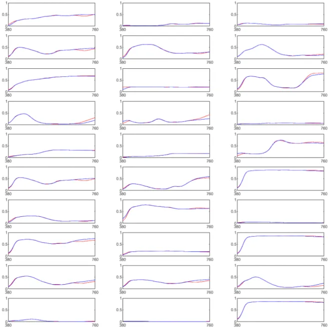
Figure 17. The measured reflectance spectra (red line) compared to the predicted reflectance spectra (blue line) calculated from the actual camera signal. ... 32

Figure 18. The measured reflectance spectra (red line) compared to the predicted reflectance

spectra (blue line) calculated using the predicted camera signal. ... 35

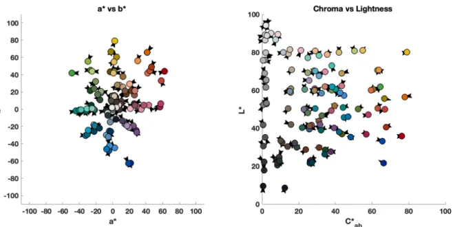
Figure 19. CIELAB a* vs. b* and L* vs. C*ab vector plots of the measured and predicted colorimetric data calculated from the actual camera signal. ... 36

Figure 20. CIELAB a* vs. b* and L* vs. C*ab vector plots of the measured and predicted colorimetric data calculated from the predicted camera signal. ... 36

Figure 21. CIELAB a* vs. b* and L* vs. C*ab vector plots of the measured and predicted colorimetric data calculated from the optimized matrix coefficients of the actual camera signal. ... 37

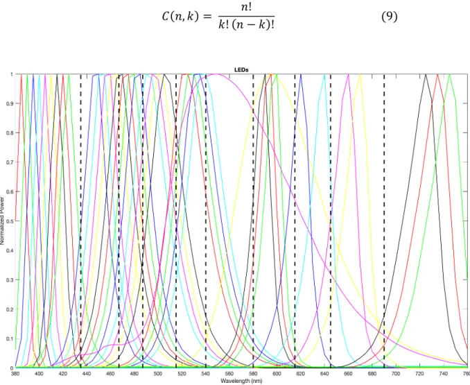
Figure 22. Normalized spectral power distributions of 37 LEDs used in the simulation. ... 40

Figure 23. Computational LED Selection simulation flow. ... 42

Figure 24. Frequency distribution of the LED lights for the Top 1000 Combinations. ... 44

Figure 25. ∆E00, Noise and RMSE of the top 1000 combinations. ... 45

Figure 26. ∆E00, Noise (∆L) and RMSE of the top 1000 combinations. ... 45

Figure 27. ∆E00 and RMSE of the top 1000 combinations. ... 46

Figure 28. Signal to Noise Ratio for Combination # 671. ... 48

Figure 29. Signal to Noise Ratio for Combination # 669. ... 48

Figure 30. Signal to Noise Ratio for Combination # 83. ... 49

Figure 31. Signal to Noise Ratio for Combination # 30. ... 49

Figure 32. The measured reflectance spectra (red line) compared to the predicted reflectance spectra (blue line) calculated from LED combination number 671. ... 52

Figure 33. The difference between the measured spectra and the calculated predicted spectra from LED combination number 671. ... 53

Figure 34. CIELAB a* vs. b* and L* vs. C*ab vector plots of the measured and predicted colorimetric data calculated from LED combination number 671. ... 53

Appendix: Figure 35. Actual measured radiance values of the LEDs from LEDmotive Technologies. ... 82

List of Tables

Table 1. Calculated R2_{, slope and y-intercept of the targets. ... 22}

Table 2. Nonlinear optimization initial and final matrices. ... 26

Table 3. Color matrix transformation optimization results. ... 27

Table 4. Peak wavelengths of the 37 available LEDs. ... 40

Table 5. Top LED combinations. ... 47

Appendix: Table 6. LEDS in LED Bin number 1 with their corresponding Spectral Power Distribution. ... 63

Table 7. LEDS in LED Bin number 2 with their corresponding Spectral Power Distribution. ... 64

Table 8. LEDS in LED Bin number 3 with their corresponding Spectral Power Distribution. ... 66

Table 9. LEDS in LED Bin number 4 with their corresponding Spectral Power Distribution. ... 67

Table 10. LEDS in LED Bin number 5 with their corresponding Spectral Power Distribution. . 69

Table 11. LEDS in LED Bin number 6 with their corresponding Spectral Power Distribution. . 71

Table 12. LEDS in LED Bin number 7 with their corresponding Spectral Power Distribution. . 72

Table 13. LEDS in LED Bin number 8 with their corresponding Spectral Power Distribution. . 74

Table 14. LEDS in LED Bin number 9 with their corresponding Spectral Power Distribution. . 76

Table 15. LEDS in LED Bin number 10 with their corresponding Spectral Power Distribution. 77 Table 16. Measured camera spectral sensitivity of the Microline ML50100 monochrome CCD camera. ... 80

Chapter 1: Introduction

Imaging as a function of wavelength is defined as spectral imaging or imaging spectroscopy. Multispectral and hyperspectral imaging are more popular terms although ambiguous. This thesis is concerned with designing an LED-based spectral imaging system with 10 channels. The cultural heritage imaging community would define this as a multispectral system. Accordingly, this term is used throughout the thesis.

The use multispectral imaging systems in cultural heritage conservation had been shown to be effective in art reproduction (Imai, F. H., Rosen, M. R., & Berns, R. S., 2001), pigment identification (Abed, F. M., 2014), pigment mapping (Zhao, Y., Berns, R. S., Taplin, L. A., & Coddington, J. , 2008), digital restoration (Easton, R. L., Christens-Barry, W. A., & Knox, K. T., 2011) etc. Renowned museums such as the Getty Conservation Institute and the Smithsonian Museum Conservation Institute have dedicated imaging departments working on multispectral imaging research for imaging of artworks and artifacts (Wong, L. and Trentelman, K., 2017; Multispectral and Hyperspectral Imaging, n.d.). The Munsell Color Science Laboratory (MCSL) and the Chester F. Carlson Center for Imaging Science Department at Rochester Institute of Technology have established research programs in multispectral imaging. A notable one from MCSL involves the development of the dual RGB system which was used in the pigment mapping of Vincent van Gogh’s The Starry Night (Zhao, Y., Berns, R. S., Taplin, L. A., & Coddington, J. , 2008). The camera used an RGB sensor and two sequential absorption filters. A second system developed at MCSL used a panchromatic sensor and seven sequential absorption filters (Burns, P. D. and Berns, R. S. , 1996; Burns, Peter, 1997; Berns, 2018; Wang, Y., & Berns, R. S. , 2017; Wang, 2016). (A review of multispectral literature is presented in Chapter 2.)

This thesis describes research to specify a third MCSL multispectral imaging system where colored LEDs replace absorption filters (Berns, R. S., 2019). LED illuminators work best for historic and light sensitive artifacts such as fragile manuscripts or old paintings because they generate light by electronic transitions instead of thermal interactions. This process gives off little to no heat to the illuminated object (Easton, R. L., Christens-Barry, W. A., & Knox, K. T., 2011). LEDs have several advantages over other illuminants such as good energy efficiency, long life span, durability, cold temperature operation, no IR or UV emissions and wide scopes of options available in the market (8 Advantages of LED Lighting, n.d.).

The Norwegian Colour and Visual Computing Laboratory at Norwegian University of Science and Technology had previously researched the development and use of LEDs in multispectral imaging system led by Dr. Raju Shrestha and Dr. Jon Yngve Hardeberg. Their work includes LED based multispectral film scanner for film digitization (Shrestha, R., Hardeberg, J. Y., & Boust, C., 2012), identifying the factors influencing a LED based multispectral imaging system (Shrestha, R., & Hardeberg, J. Y. , 2013; Shrestha, R., & Hardeberg, J. Y. , 2014), LED matrix design for multispectral imaging system (Shrestha, R., & Hardeberg, J. Y., 2013) and the comparison of LED based multispectral imaging system against a filter based multispectral imaging system and a hyperspectral imaging system (Shrestha, R., & Hardeberg, J. Y., 2018). The said works helped in pinpointing the metrics (∆E00, Goodness of Fit Coefficient and Root mean

square error) to be used in evaluating the colorimetric and spectral accuracy in the LED-based multispectral imaging system proposed in this thesis. Furthermore, they showed that the LED-based multispectral imaging system composed of six LEDs performed better than a filter-LED-based multispectral imaging system and was as good as the hyperspectral imaging system (Shrestha, R., & Hardeberg, J. Y., 2018). Of course, the quality and performance of the filter-based spectral imaging system used in (Shrestha, R., & Hardeberg, J. Y., 2018) can be improved by increasing the number of channels and the use of a more refined camera.

The thesis is subdivided into two sections. The first part involved the evaluation of a camera model in predicting the signals of a LED illumination system coupled with a panchromatic camera. The 10 LEDs were chosen by the manufacturing company with the goal of well simulating conventional lighting. The second part dealt with the computational selection of LEDs using the spectral data from the 37 LED lights available from the manufacturer. The computational selection performed an imaging simulation in order to determine the best LED set composed of 10 LEDs. The optimal set can be used to specify a custom Spectra Tunelab source. The Euclidean method and Score ranking method were used in order to determine the best LED combination. Imai et. al (2002) showed that no metric is superior over others and so it was recommended to use a combination of metrics in order to gain the advantage of each metric (Imai, F.H.; Rosen, M.R.; Berns, R.S., 2002). The ideal combination would yield good colorimetric accuracy, good spectral accuracy and low image noise. Future works involves the purchase of the LEDs chosen from the computational selection to build the LED-based multispectral imaging system and comparison of the results from the computational imaging simulation to the actual imaging experimentation.

Chapter 2: Review of Related Literature

2. Multispectral Imaging System

A multispectral imaging system captures data within the specified region of interest across the electromagnetic spectrum. The multispectral image produced is usually created with multiple bands of wavelengths collected using narrow-band LED illumination or colored filters placed between the object and the sensor (Berns, R. S., 2019). Each channel yields spectral information that is uniquely present only in the specified wavelength region. For example, a certain pigment in an artwork cannot be detected in the visible spectrum but can be detected in the infrared region. As such, increasing the number of channels yields more spectral information (Wang, Y., & Berns, R. S. , 2017; Dickinson, C. , 2001). Bear in mind that creating such systems increases cost and complexity. Berns (2005) discussed a trade-off between spectral accuracy, colorimetric accuracy, cost, and hardware and software complexity. Most multispectral imaging systems use monochrome cameras. An ideal multispectral imaging system would have good colorimetric accuracy, good spectral accuracy, and low image noise (Berns, Roy S., 2005).

A schematic representation of a multispectral imaging system and a multispectral image is shown in Figure 1. Figure 1a shows a filter-based multispectral imaging system, showing a filter wheel in front of a camera. In a LED-based multispectral imaging system, the filter-wheel is removed, and LED illuminants are used. Figure 1b shows the multispectral data cube containing multiple channels.

2.1. Applications in Cultural Heritage Conservation

Multispectral imaging has significant applications in military, medicine, remote sensing and cultural heritage conservation (Coffey, Valerie C., 2012). This thesis focuses on the application of multispectral imaging in cultural heritage conservation. Some application of multispectral imaging in cultural heritage conservation includes pigment identification (Zhao, Y., Berns, R. S., Taplin, L. A., & Coddington, J. , 2008), spectral based color-reproduction of artwork (Berns, R. S., Imai, F. H., Burns, P. D., & Tzeng, D. Y., 1998; Imai, F. H., Rosen, M. R., & Berns, R. S., 2001) and reconstruction of ancient manuscripts (Hansen, D. Michael, 2006). The Munsell Color Science Laboratory and the Chester F. Carlson Center for Imaging Science at Rochester Institute of Technology have established research programs in the development of multispectral imaging in cultural heritage conservation. Past and current on-going research are described below.

2.1.1. The Development of Multispectral Imaging at the Munsell Color Science

Laboratory

A spectral-based color reproduction system using multispectral imaging was developed at the Rochester Institute of Technology-Munsell Color Science Laboratory around 1998 by Dr. Roy Berns and Dr. Francisco Imai (Berns, R. S., Imai, F. H., Burns, P. D., & Tzeng, D. Y., 1998). In 2001, the effectiveness of multi-channel visible-spectrum imaging was demonstrated in creating the least metameric reproduction of a van Gogh target with reasonable colorimetric and spectral accuracy. The researchers made use of two approaches in capturing the images. A wide-band capture approach was applied using a conventional camera and Kodak Wratten filters. This showed a less satisfactory result than a narrow-band approach using a liquid crystal tunable filter (LCTF). Imai et. al (2000) published a comparison of two imaging techniques. The wide-band is less time consuming and more applicable to colorants having wide-band spectral features while narrow-band does not require prior knowledge of the colorants used in the artwork and registration and calibration artifacts are not an issue (Imai, F. H., Rosen, M. R., & Berns, R. S., 2001; Imai, F. H., Rosen, M. R., & Berns, R. S., 2000). A collection of pigments researched to be in the actual van Gogh Self-portrait painting was used in the creation of the target. The effectiveness was evaluated by comparing the estimated spectral reflectance derived from the eigenvector analysis against the measured spectral reflectance from a spectrophotometer. The reflectance spectra of the printed reproduction of the van Gogh target was measured and compared to the measured reflectance of

the target in order to evaluate the accuracy of the spectral-based printing system. For colorimetric accuracy, the system showed a ∆E*94 of 5.0 and for spectral accuracy, a 3.1% RMSE (Imai, F. H.,

Rosen, M. R., & Berns, R. S., 2001).

Another notable example of the application of multispectral imaging in the field of cultural heritage conservation was the pigment mapping of Vincent van Gogh’s The Starry Night. Zhao et. al (2008) made use of the dual RGB system developed in the Munsell Color Science Laboratory. A Color-Filter-Array (CFA) camera combined with two optimized filters was used to capture the two RGB images assembled to a six-channel spectral image. The two green channels are nearly identical thus only five channels are used for spectral reconstruction. To preserve high colorimetric accuracy, a spectral reconstruction method that combines spectral and colorimetric transformations was used together with the system to retrieve pixel by pixel spectral reflectance factor (Wang, Y., & Berns, R. S. , 2017; Zhao, Y., Berns, R. S., Taplin, L. A., & Coddington, J. , 2008; Berns, R., Taplin, L., & Nezamabadi, M., 2005; Berns, R., Taplin, L., & Nezamabadi, M., 2004). The same calibration target used in Imai et. al (2001) was used in pigment mapping of Vincent van Gogh’s

The Starry Night. A calibration target is needed in order to use the method which in the case of pigment mapping of Vincent van Gogh’s The Starry Night was readily available from the past publication (see (Imai, F. H., Rosen, M. R., & Berns, R. S., 2001)). The Matrix R method was used in the pigment mapping as well, it is a type of learning-based reconstruction developed through Wyszecki’s hypothesis and Cohen and Kappauf’s Matrix R theory (Zhao, Y., & Berns, R. S., 2007). Matrix R theory is a spectral decomposition derived from Wyszecki’s hypothesis that a ‘‘fundamental stimulus’’ and a ‘‘metameric black’’ can be derived from decomposing a “color stimulus” into two spectra (Wyszecki, G. , 1953).

In addition to the Matrix R method, Kubelka-Munk (K-M) theory was applied to map the pigments in van Gogh’s The Starry Night. K-M theory was used to predict the spectral reflectance of the pigment mixture using the individual measured reflectance of the pigments used to create the mixture (Berns, R. S., 2019; Abed, F. M., 2014; Walowit, E., Mccarthy, C. J., & Berns, R. S. , 1987). Each pixel is matched with the most probable pixel based on the predicated values from the K-M calculations. The map is then created from the accumulated matched pigments.

In summary, the effectiveness of the pigment mapping technique depends on the prior knowledge of the artist’s palette. However, the availability of a universal target works as well for

deriving the eigenvectors needed to estimate the spectra (Imai, F. H., & Berns, R. S., 2002). The study was able to map-out seven out of 10 paints from the artist’s palette.

Some more current research at MCSL for multispectral imaging in cultural heritage conservation involves digital reproduction of artwork via a computer graphics rendering tool combined with a modified photometric stereo technique (Cox, B. D., & Berns, R. S., 2015), imaging using an affordable single, commercially available mirrorless digital camera (Kuzio, O., & Berns, R. S., 2019) and now the development of an LED-based multispectral imaging, the subject of this thesis.

2.1.2 Multispectral Imaging of Archimedes Palimpsest at Chester F. Carlson

Center for Imaging Science

Research regarding multispectral imaging of Archimedes palimpsest at Chester F. Carlson Center for Imaging Science had been on-going since 2000. The goal of the research is to recover Archimedes’ original written text that was erased and overwritten with the Euchologion (a Christian prayer book). Such a document is known as a palimpsest. In addition to the overwriting done by 13th _{century Christian monks, forged pictures were also added that hid more of its written}

texts. Improper handling and storage led to the further degradation of the pages of the palimpsest making its text more undiscernible. The palimpsest provides an insight into Archimedes’ works and the progress of mathematics and physics in 3rd _{century BCE. The Archimedes Palimpsest}

contains seven treatises of Archimedes. These are, “On the Equilibrium of Planes", "Spiral Lines", "Measurement of a Circle", "On the Sphere and Cylinder", "On Floating Bodies", "The Method of Mechanical Theorems" and "Stomachion", all of which proves how Archimedes was way ahead of his time (The Archimedes Palimpsest, n.d.; Netz R., and Noel W., 2007.).

Several imaging techniques were tried in order to meet the goal. Initial imaging involved the use of least-squares spectral unmixing, where the components of the images were categorized into overwriting, underwriting, parchment and mold. The images were captured using a 12-bit scientific camera coupled with five glass filters transmitting light from ultraviolet to infrared region with widths of 100 nm. In addition to, three illuminants were used (visible light, shortwave ultraviolet lamps and longwave ultraviolet lamps). This subsequently produced 15 spectral images processed using the least-squares spectral algorithm. This was done to strip off the prayer book and reveal the undertext palimpsest. The technique was successful in stripping off much of the ink

from the prayer book however it also removed some underwriting that were overlaid by the inks from the prayer book leaving gaps making the palimpsest more unreadable (Easton, R., & Knox, K., 2004; Walvoord, D. J., & Easton, R. L., 2008; Easton, R. L., Christens-Barry, W. A., & Knox, K. T., 2011; Knox, K. T., Dickinson, C., Wei, L., Easton Jr, R. L., & Johnston, R. H., 2001; Easton, R. L., Christens-Barry, W. A., & Knox, K. T, 2011).

In order to solve this dilemma, the researchers deemed it more appropriate to just retain the overwriting but have it less visible and fainted in the background by increasing the contrast and appearance of the original underwriting. Images of the pages were captured under varying LED illuminants ranging from short wavelength to long wavelength. The LED illumination system called “Eureka Lights” was composed of one waveband (λ ~ 365nm) in the UV region, seven in visible region (λ~ 445nm, 470nm, 505nm, 530nm, 570nm, 617nm, and 625nm) and three in infrared region (λ ~ 700nm, 735nm, and 870nm). It was seen that the underwriting fades more with an increase in wavelength, thus imaging it under ultraviolet illumination was the best choice. The pseudo-color technique was then applied by assigning specific colors for the four categories (overwriting, underwriting, parchment and mold). The resulting image showed a red text for the underwriting and a neutral gray or black for the unwanted text. This contrast helped the scholars in deciphering the texts in the intact portions of the palimpsest, however the moldy sections and the degraded pages are still problematic (Hansen, D. Michael, 2006; Walvoord, D. J., & Easton, R. L., 2008; Easton, R. L., Christens-Barry, W. A., & Knox, K. T., 2011; Knox, K. T., Dickinson, C., Wei, L., Easton Jr, R. L., & Johnston, R. H., 2001; Knox, K. T., 2008).

For the degraded and moldy portion of the palimpsest, the researches made use of a character recognition method. This method makes use of a training library built from the transcribed portions of the palimpsest. The method yields a list of probable words that matches the character fragment and then are further evaluated by the scholar to see if the word makes coherent sense in the palimpsest (Walvoord, D. J., & Easton, R. L., 2008; Easton, R. L., Christens-Barry, W. A., & Knox, K. T., 2011; Walvoord, D. J. , 2008). In addition to Perry et. al (2018) implemented the use of two-dimensional flattening on damaged and distorted documents (Peery, T. R., & Messinger, D., 2018). The research aimed to develop and enhance the training technique in order to be applied to the damage portions of the palimpsest. The technique aimed to digitally unravel or flatten warped objects such as scrolls damaged by fire, water or other force of nature. The study showed that flattening in sections then assembling these images rather than doing the whole

document yielded better results. Furthermore, although the flat to sharp method required fewer steps, the method yielded less spectral error (Peery, T. R., & Messinger, D., 2018).

Perry et. al (2018) also published a study comparing the currently available multispectral imaging at the Chester F. Carlson Center for Imaging Science to a hyperspectral imaging system (HSI) available at the University of Rochester in terms of noise. Although hyperspectral imaging systems was seen to have spectral/spatial compromise unlike a multispectral imaging system, a lower quality system would still meet the requirement if the application of the system heavily depends on human vision. An example would be the transcribing of a palimpsest which is done within the limits of the human visual system. A finer higher resolution image beyond what is detectable or needed to read the text is unnecessary (Peery, T. R., & Messinger, D., 2018; Peery, Tyler R., 2019). Furthermore, panchromatic sharpening was seen to be effective in recovering the decrease in spatial resolution compared with hyperspectral imaging (Peery, T. R., & Messinger, D. W. , 2019).

In summary, a variation and a combination of imaging techniques is needed for the different portions of the palimpsest. The condition of the palimpsest and the demands of the scholars who transcribed the texts heavily influenced the imaging technique used.

2.2 LED based-Multispectral Imaging System

This thesis aims to develop a LED-based multispectral imaging system. The use of LEDs instead of filters is another way of doing multispectral imaging. In this approach, an image is captured using a monochrome camera for each LED light. These set of n images captured under the set of n lights is combined to produce the n-channel multispectral image (Park, J.I., Lee M.H., Grossberg M.D.Z.D., and Nayar S.K.).

The rise of the manufacturing industries of LED nowadays lead to the increase in options, availability and cost effectiveness (Shrestha, R., & Hardeberg, J. Y., 2013). LED based multispectral imaging research had been shown to have important application in film digitization (Shrestha, R., Hardeberg, J. Y., & Boust, C., 2012), digital color proof in print reproduction (Yamamoto, S., Tsumura, N., Nakaguchi, T., & Miyake, Y., 2007), cultural heritage conservation (Shrestha, R., & Hardeberg, J. Y. , 2013), and medical imaging (Everdell N. L., Styles I. B., Claridge E., Hebden J. C., and Calcagni A. S. , 2009), among others. Light generated from LEDs apply little to no heat, which is vital in the imaging of fragile historical documents or artworks.

The availability of narrow-band LEDs is also good for spectral image processing (Easton, R. L., Christens-Barry, W. A., & Knox, K. T., 2011). The researchers are particularly interested in the application of multispectral imaging in cultural heritage conservation. Previous studies relating to LED-based multispectral imaging are discussed below.

Shrestha and Hardeberg (2014) determined four major factors that affect the performance of multispectral imaging using LEDs: camera type, demosaicing method, the number of LEDs, and noise. LED based multispectral imaging simulations using a monochrome camera and an RGB camera were performed. The simulation made use of two sets of LED lights: the first set was composed of 19 LED that were previously used in the development of a LED based multispectral film scanner (see (Shrestha, R., Hardeberg, J. Y., & Boust, C., 2012)) and the other set was composed of 6 LEDs fromJUST Normlicht LED Color Control light booth. The spectral power distribution (SPD)of the two sets of LEDs are shown in Figure 2. The spectral power distributions of the LEDs were uniformly distributed throughout the visible spectrum. Shrestha and Hardeberg simulated six and nine band systems as what were previously found to be the constrained range of the number of LEDs in this system in their previous research (see (Shrestha, R., Hardeberg, J. Y., & Boust, C., 2012)).

Figure 2. Spectral power distribution of the two sets of LEDs used in Shrestha and Hardeberg (2014).

The results showed that the nine-band system using a monochrome camera performed the best with an RMS error of 0.011 while the two six-band systems using the monochrome camera and the RGB camera performed the same. Noise was investigated as well by introducing a random

gaussian noise of about 0% to 20%. As expected, the amount of noise is directly proportional to the RMS error and also to the increase in the number of LEDs used. Although the RGB camera speeds up the image capturing process, the necessary demosaicing had an impact on the spatial accuracy thus affecting the quality of the images (Shrestha, R., & Hardeberg, J. Y. , 2014; Shrestha, R., & Hardeberg, J. Y., 2013). The use of a monochrome camera combined with a large selection of LEDs covering the range of the electromagnetic spectrum was ultimately recommended (Shrestha, R., & Hardeberg, J. Y. , 2014).

This thesis starts with the computational selection of the LEDs for multispectral imaging. LED selection plays a vital role in constructing and designing a LED-based multispectral imaging system. The number of LEDs corresponds to the number of channels, as such the image quality, spectral accuracy and colorimetric accuracy heavily depends on the number of LEDs and its region of interest in the electromagnetic spectrum. The maximum number of LEDs that can be used in the system is usually restricted by cost and manufacturing limitations (Shrestha, R., Hardeberg, J. Y., & Boust, C., 2012). Previous researches regarding LED selection and filter selection provided valuable insights for the selection process in this research (Shrestha, R., Hardeberg, J. Y., & Boust, C., 2012; Wang, Y., & Berns, R. S. , 2017; Li, S. X., 2018).

Wang et. al (2016) made use of fitting Gaussians method and a traditional subsets selection method in choosing the best filter for wide-band multispectral imaging. Narrow-band was deemed to be unfit for cultural-heritage studio imaging due to its complex image registration, costly customized filters and time-consuming measurements. An imaging simulation was performed using the Schott filter spectral database and the current filters sold by the Andover Corporation. The fitting Gaussian method is a method of choosing seven filters that were the closest to the theoretical Gaussian filters while the traditional selection method involved dividing the LED sets according to their region of interest then running the simulation and sorting according to the computed colorimetric and spectral accuracy. The study showed that fitting Gaussian method was better compared to the traditional selection method utilizing less computational time and better results. The fitting Gaussian method yielded a noise of 1.08, ∆E00 of 0.28, RMS of 0.019 in

comparison to the selection method who’s top 1000 combinations yielded noise of less than 1.60, ∆E00 larger than 0.7 and RMS in the range of 0.022-0.024. The researchers then chose the filters

Li (2018) had a similar approach to Shrestha et. al (2012) in the use of metrics such as Root mean square error and Goodness of Fit Coefficient (Shrestha, R., Hardeberg, J. Y., & Boust, C., 2012) and made use of the maximum linear independent (MLI) filter selection method. The spectral data of 45 broadband filters (400-700 nm) from Hoya manufacturing was used in the imaging simulation. An optimal filter set is selected via a filter vector analysis. The metrics chosen determined the optimal filter set. The results of the simulation showed that the chosen filter set had five-channels with a uniform peak distribution in its transmittance curves, overlapped transmittance curve with the adjacent filter and a distinct transmittance peak in its first filter.

Based on the study of Imai et. al (2002), there was not a metric that was conclusively superior over others for all purposes. As such it was recommended to use a combination of the metrics in order to gain the advantage of each metric (Imai, F.H.; Rosen, M.R.; Berns, R.S., 2002). The metrics chosen in this thesis are discussed in detail in the following chapters.

Chapter 3: Verifying the Camera Model

Preliminary experiments to verify the camera model and evaluate the currently available LEDs at Munsell Color Science Laboratory (MCSL) are discussed below. The chapter is divided into parts to describe the imaging system composed of 10 LEDs and a monochrome camera and the calculations performed to evaluate the colorimetric and spectral accuracy of the imaging system. The calculation includes the use of the actual camera signal taken from the images and the calculated predicted camera signal.

3.1 Multispectral Imaging Workflow

The workflow for multispectral imaging process is shown in Figure 3. The images captured under each light were flat fielded and registered. (Dark current subtraction was performed automatically in the camera software.) Flat fielding is needed to correct the non-uniformity in the images due to the pixel to pixel gain variation of the sensor, nonuniform lighting and light fall off caused by the lens (Li, S. X., 2018; Kalajian, P. , 2011).

Image registration is needed due to the variation in the camera focus for each LED light. The image registration helped in reducing the difference in magnification and the shift in imaging caused by chromatic aberration. MATLAB’s Speeded-Up Robust Features (SURF) registration was used in this thesis (MathWorks, n.d.). SURF is a feature detector algorithm that detects feature-points in an image. These features could be corners, blobs, lines, edges etc. In a study conducted by Tareen and Saleem in 2018 comparing various feature detector algorithms, SURF was seen to detect more features than other algorithms (SIFT, AKAZE, KAZE) (Tareen, S. A. K., & Saleem, Z., 2018). The variation in camera focus in each LED light and the consequent image registration wasn’t as big of a challenge in multispectral imaging using LED light compared to multispectral imaging using filters with varying thickness. The Sky X professional software by Software Bisque Inc had automatic focusing function that helped determined the best focus during the imaging. The variation in camera focus value under each LED light ranged from 0-1 %. The chosen reference image was the image taken under the LED whose peak sensitivity was nearest to V(λ). Lastly, the images were evaluated according to image quality, colorimetric accuracy and spectral accuracy.

An illustration of the imaging system is depicted in Figure 4 and the actual set up is shown in Figure 5. The imaging system is composed of a Finger Lakes Instrumentation Microline ML50100 monochrome CCD camera, Rodenstock HR Digaron-S 4.0/100 mm with Copal shutter, and 10 LEDs from LEDmotive Technologies. A more detailed description of the instruments used is provided in the following sections.

Figure 3. Workflow of multispectral imaging.

Figure 4. Illustration of the imaging system.

Capturing an image under each light

Flat-fielding of the captured images

Image Registration

Evaluating the results according to image quality, colorimetric accuracy and spectral accuracy

Figure 5. LED-based multispectral imaging at Munsell Color Science Laboratory- Rochester Institute of Technology.

3.2 The Imaging System

The camera sensitivity of a Microline ML50100 monochrome CCD camera manufactured by Finger Lakes Instrumentation with attached lens was measured using a Newport Cornerstone monochromator. The set-up of the camera sensitivity measurement is seen in Figure 6. The measurement was done in a dark room. The Newport Cornerstone monochromator was controlled by MATLAB. The lamp was warmed-up 10 minutes prior to the measurement. The monochromator was adjusted at levels 1-3, (1)330-600 nm, (2)600-800 nm and (3) 800-1100 nm in accordance to the wavelength being measured. The radiance was measured from 400-760 nm with increments of 10 nm using a Photo Research PR-655. The values were then interpolated to produce increments in 1 nm data.

Images at each wavelength were captured taking a great care to make sure the images were not overexposed. Given that the tiff images were too large and takes a large amount of time to load and process, only the values on the chosen certain portion of the image were used in the calculation

(see Figure 7). Furthermore, only the image containing the light is needed, and so selecting a certain portion is an easier and a faster way. There were 204x245 pixels selected. The mean digital counts were then divided by their corresponding radiance. The black background was subtracted automatically by the Sky X professional software.

The Sky X professional software by Software Bisque Inc. was used to control the camera. The software proved to be very useful in providing automatic dark subtraction, camera temperature control and computer-aided focusing.

The camera is a 16-bit 50.1-megapixel camera that operates using a KAF-50100 Image Sensor. The said camera’s sensitivity was used in the verification of the camera model and the computational imaging simulation. The camera relative spectral sensitivity of the monochrome camera is shown in Figure 8.

Figure 6. Newport Cornerstone monochromator, Microline ML50100 monochrome CCD camera and Photo Research PR-655 set up. (Disclaimer: The picture was shot in a well-lit room

for the sake of clearly showing the set-up; the entirety of the experiment occurred in a dark room). Monochromator Monochrome CCD Camera PR-655 Integrating _Sphere Arc Lamp Monochromator Level Dial

Figure 7. The box in the 540 nm image shows the area for which the values were extracted, 204 by 245 pixels.

Figure 8. Microline ML50100 camera spectral sensitivity normalized to unity at peak height.

The LED system used in this thesis is made by LEDmotive Technologies (see Figure 9 for the actual model). The spectra tune lab device is composed of 10 LEDs with varying peak

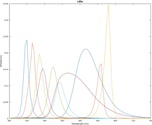
wavelengths from 430-660 nm, specifically 430 nm, 445 nm, 465 nm, 475 nm, 505 nm, 520 nm, 545 nm, 595 nm, 640 nm and 660 nm. The manufacturer’s data of the spectral power distribution of the LEDs is shown below in Figure 10. The LEDs were measured again in the lab using Photo Research PR-655, the measured radiance was rescaled and plotted for comparison as shown in Figure 11. The LEDs were embedded within the device and were controlled using the LEDmotive µWAVE software. As of now the software only runs in a Windows OS. The software is capable of delivering either a single monochromatic light or a combination of these lights. The lights require no warm-up time and can be dimmed from 0% - 100% per channel with a resolution depth of 12 bits (4096 steps) (LEDMOTIVE, n.d.). A Godox standard 7” reflector was attached to the front of the light source.

Figure 9. Spectra Tune Lab front and rear view (accessed on March 2020, https://ledmotive.com).

Figure 10. Spectral power distribution of the LEDs from LEDmotive Technologies.

Figure 11. Measured spectral radiance of the LEDs from LEDmotive Technologies.

380 430 480 530 580 630 680 730 780 Wavelength (nm) 0 0.005 0.01 0.015 0.02 0.025 0.03 0.035 Relative Power LEDs

3.3 The Target

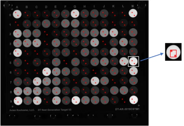
The imaging made use of DT Next Generation Target V2 made by Avian Rochester, L.L.C. It is composed of 130 patches. The target was modified to include pigments such as bone black, lead white, titanium white, ultramarine, cobalt blue and chromium oxide green. The said pigments were popular in artist’s palette. For example, lead white is a popular white pigment in old master paintings before it was replaced by titanium white in the 20th _{century (Fortunato, 2005). Modifying}

the target to include historical pigments is important in multispectral imaging of paintings. The reflectance of the target was measured using an i1 Pro 2 X-rite spectrophotometer using 45°a/0° geometry as seen in Figure 12.

3.4 Camera Signal

The camera signal represents the measured amount of light from the image, which is the number of electrons captured by the CCD or the number of counts present in the captured image (Clark, R., n.d.). In multispectral imaging, the camera signal is taken as the mean pixel value in the specified area, for which in the case of the Next Generation Target is the area of each patch. As seen in Figure 13 below, around 60% of the patch was used to determine the camera signal. The red asterisk determines the border of the camera signal taken; lines connecting the asterisk forms a rectangle, clearly showing the actual area of the patch.

Figure 13. Sample image of a target showing marked areas where camera signals were averaged.

Aside from the data using the captured images, the camera signal was predicted. The camera signal c was calculated using the Equation 1 below, where S defines the spectral sensitivity of the monochrome camera, E represents the LEDs spectral power distribution (SPD) and R is the reflectance measurements of the DT Next Generation Target V2.

where

The linear relationship of the actual camera signal and the predicted camera signal is shown in Figure 14. Regression analysis showed that the 130 patches follows an excellent linearity with R2 _{of 0.99. The linear fit showed a slope of 1.0-1.1 and y-intercepts < 0.01 for the targets (see}

Table 1 for the calculated slope, R2 _{per target and y-intercept). These show that the camera model}

predicted the camera signals well. The difference between the predicted cameral signal and the actual camera signal from the images are small and unbiased. Unbiased in this context means that the predicted camera signals were found to be in a reasonable range (not too high or too low) around the measured values (Frost, J., n.d.).

S= s_λ,1 ... s_λ,1 ! ... ! s_λ,n ... s_λ,n ⎛ ⎝ ⎜ ⎜ ⎜ ⎜ ⎞ ⎠ ⎟ ⎟ ⎟ ⎟ , E= E_λ 0 0 0 ! 0 0 0 E_λ ⎛ ⎝ ⎜ ⎜ ⎜ ⎜ ⎞ ⎠ ⎟ ⎟ ⎟ ⎟ , R= R_λ,1 ... R_λ,i ! ... ! R_λ,1 ... R_λ,i ⎛ ⎝ ⎜ ⎜ ⎜ ⎜ ⎞ ⎠ ⎟ ⎟ ⎟ ⎟ ,

Figure 14. Actual and Predicted Camera Signals. Table 1. Calculated R2_{, slope and y-intercept of the targets.}

Target R2 _{Slope Y-intercept}

1 0.99 1.0 1.4 x 10-2 2 0.99 1.0 -4.5 x 10-4 3 0.99 1.0 7.5 x 10-4 4 0.99 1.1 1.0 x 10-3 5 0.99 1.0 8.0 x 10-4 6 0.99 1.0 2.6 x 10-3 7 0.99 1.0 4.5 x 10-3 8 0.99 1.0 3.6 x 10-3 9 0.99 1.0 4.3 x 10-3 10 0.99 1.0 6.2 x 10-3

The camera signal was then used to predict the spectral reflectanceof the patches. Equation 2 below shows the derivation of the spectral reflectance R using the spectral transformation matrix MS coefficients multiplied to the camera signal c. The matrix was derived using Equation 3, as the

product of the pseudoinverse (MATLAB pinv) of the cameral signal c+_{and the measured spectral}

reflectance R values of the calibration target (Berns, R. S., 2019; Zhao, Y., & Berns, R. S., 2007). Root-mean-square-error (RMSE) was used as the metric for the reflectance spectral accuracy. .

𝐑 = 𝐌𝑺𝐜 (2)

𝐌_𝑺 = 𝐑𝐜" ₍₃₎

The tristimulus values t can be computed from the reflectance values R using Equation 4 below. The result is the same as the predicted tristimulus values from the camera signal using Equation 5. The T represents the color matching functions of the observer, the S is the spectral power distribution of the illuminant and R is the reflectance values of the target.

𝐭 = 𝐓𝐒𝐑 (4) where, 𝐭 = 0 𝑋_# 𝑌_# 𝑍_# … … … 𝑋_$ 𝑌_$ 𝑍_$5

The camera signal can also be used to predict the tristimulus values of the patches. Equation 5 below shows the derivation of the tristimulus values t using the color transformation matrix MT

coefficients multiplied to the camera signal c. The matrix MT was derived using Equation 6, as the S= S_λ 0 0 0 ! 0 0 0 S_λ ⎛ ⎝ ⎜ ⎜ ⎜ ⎜ ⎞ ⎠ ⎟ ⎟ ⎟ ⎟ ,T_xyz = x_λ ... x_λ y_λ ... y_λ z_λ ... z_λ ⎛ ⎝ ⎜ ⎜ ⎜⎜ ⎞ ⎠ ⎟ ⎟ ⎟⎟

product of the pseudoinverse (pinv) of the cameral signal c+ _{and measured tristimulus values tof}

the calibration target (Berns, R. S., 2019; Berns, R., Taplin, L., & Nezamabadi, M., 2005). Estimated tristimulus value are the same using Equations 5 or 6 since the relationship between spectral reflectance and tristimulus values are linear.

𝐭 = 𝐌_𝑻𝐜 (5)

𝐌_𝑻 = 𝐭𝐜" ₍₆₎

CIEDE2000 was used as the metric for colorimetric accuracy with the positional function, SL, equal to unity (see Equation 7); doing this gives more significance to the lightness noise that

is more visible in an image (Berns, R., 2016). Noise represents the uncertainty in the signal (Burns, Peter, 1997). This is usually seen as a variation in lightness or color in the images. Noise is usually brought about by several factors such as exposure shot noise, instrument error due to deterioration of the imaging device or calibration variation, error propagation occurring during the transformation of the image signals, etc. (Burns, P.D., and Berns, R.S., 1997; Burns, P.D., 2002). This thesis discusses the noise due to the color transformation (MT). Noise can be determined by

computing the standard deviation in the chosen area in an image (Noise in photographic images, 2020). It can also be computed using Equation 8 below. Previous researches made by Burns and Berns tackled the color transformation noise produced during multispectral imaging. The use of multivariate error-propagation analysis to color signal transformation proved to be helpful in modelling noise due to color measurement uncertainty in CIELAB path (Burns, P.D., and Berns, R.S., 1997; Burns, P.D., and Berns, R.S., 83-85). Kuniba and Berns followed up with a study on the design of digital camera color filters with high color accuracy and low image noise. The noise parameter, N, as shown in Equation 8, was used to evaluate the photon shot noise component among CMY filters and RGB filters. Photon shot noise is the uncertainty in the photon counting at the sensor (Kuniba, H., & Berns, R.S., 2008; Kuniba, H., & Berns, R.S., 2009). A comparison with CMY filters and RGB filters showed that RGB filters performed better in terms of color reproduction and noise despite the CMY’s capability to collect more photons. The noise during

the color transformation affected the performance of the CMY filters (Kuniba, H., & Berns, R.S., 2009).

The sum of the rows in the matrix in Equation 8 were rescaled to unity before the calculation. The equation is derived in a gray world idea where captured images assimilate to medium gray. It made use of a gray sample under illuminant E (equal-energy spectrum) and where CIELAB and CIEDE2000 total color differences are the same at L*=50.

where,

The matrix MT can be further optimized to improve the average color difference ∆E00

(SL=1). The MATLAB nonlinear optimization function fminunc was used to optimize the matrix

MTand minimize theaverage color difference ∆E00 (SL=1). The MATLAB function fminunc finds

the minimum of unconstrained multivariable function (MathWorks, n.d.). The starting pseudoinverse matrix from the actual and predicted camera signal served as the starting values while the offsets starting value was at 0. The fminunc yield better matrix coefficients with a lower average color difference ∆E00 (SL=1) of 0.89. Maximum iterations and maximum function

ΔE₀₀= Δ ′L k_LS_L ⎛ ⎝⎜ ⎞ ⎠⎟ 2 + Δ ′C k_CS_C ⎛ ⎝⎜ ⎞ ⎠⎟ 2 + Δ ′H k_HS_H ⎛ ⎝⎜ ⎞ ⎠⎟ 2 +R_T Δ ′C k_CS_C ⎛ ⎝⎜ ⎞ ⎠⎟ Δ ′H k_HS_H ⎛ ⎝⎜ ⎞ ⎠⎟ N =

( )

( )

( )

( )

(

)

( )

(

)

(

)

(

)

( )

(

)

(

)

(

)

evaluations were set at 30,000 and even at a setting higher than that, the optimized matrix remained the same. For fminunc, convergence can occur at a local minimum rather than true minimum, as such the average color difference ∆E00 (SL=1) of 0.89 is probably the minimum value. The

optimization also resulted in a lower noise of 8.0 from 8.2, a noticeable decrease in a* _{noise and}

90th _{percentile was also seen (see Table 3).}

As for the predicted camera signal, the optimization yields the same average color difference ∆E00 (SL=1) of 0.15, the optimized matrix coefficients did not change (at one significant

figure). Thus, the average color difference ∆E00 (SL=1) of 0.15 is likely the minimum value. The

noise also stayed the same for the optimized matrix coefficients.

The pseudo-inverse initial and optimized matrix coefficients are shown in Table 2. Their corresponding calculated total-color-difference statistics and transformation noise are shown in Table 3.

Table 2. Nonlinear optimization initial and final matrices.

Pseudoinverse matrices Matrix Coefficients Pseudoinverse initial matrix using actual camera signal ⎝ ⎜ ⎛0.28 0.16 0.43 0.0 −0.75 −0.59 −0.67 0.0 2.3 1.9 2.6 0.0 −2.0 −1.8 −2.0 0.0 0.64 0.63 0.68 0.0 −0.74 −0.61 −0.56 0.0 1.2 1.7 0.58 0.0 −0.14 −0.59 −0.42 0.0 0.17 0.10 0.06 0.0 −0.07 −0.07 0.02 0.0 ⎠ ⎟ ⎞ Pseudoinverse initial matrix using predicted camera signal ⎝ ⎜ ⎛−0.03 −0.04 0.11 0.0 0.320.19 0.26 0.0 −0.64 −0.47 0.19 0.0 0.54 0.38 0.12 0.0 −0.22 −0.10 0.04 0.0 0.14 −0.02 −0.02 0.0 0.19 1.22 0.04 0.0 0.56 −0.24 −0.04 0.0 0.16 0.09 0.02 0.0 −0.19 −0.14 −0.02 0.0 _⎠ ⎟ ⎞ Pseudoinverse final matrix using actual camera signal ⎝ ⎜ ⎛ 0.27 0.18 0.45 2.5 x10!" −0.70−0.60 −0.65 −1.4 x10!# 2.3 2.0 2.6 −1.1 x10!# −2.0 −1.8 −2.0 1.0 x10!# 0.55 0.54 0.69 8.2 x10!$ −0.74 −0.55 −0.58 −4.6 x10!# 1.4 1.7 0.57 −1.2 x10!# −0.18 −0.56 −0.36 9.1 x10!$ 0.21 0.14 0.06 3.9 x10!# −0.13 −0.13 −0.03 −2.6 x10!#_⎠ ⎟ ⎞ Pseudoinverse final matrix using predicted camera signal ⎝ ⎜ ⎛ −0.03 −0.04 0.11 −2.0 x10!" 0.320.19 0.26 −6.0 x10!" −0.64 −0.47 0.19 −1.7 x10!" 0.54 0.38 0.12 −4.1 x10!" −0.22 −0.10 0.04 −9.1 x10!%& 0.14 −0.02 −0.02 −5.2 x10!' 0.19 1.22 0.04 −1.0 x10!" 0.56 −0.24 −0.04 −1.2 x10!" 0.16 0.09 0.02 −9.7 x10!$ −0.19 −0.14 −0.02 1.1 x10!"_⎠ ⎟ ⎞

Table 3. Color matrix transformation optimization results.

Metric Actual Camera Signal Predicted Camera

Signal Before Optimization Average _{1.0 0.15} 90th _percentile 1.9 0.30 noise 4.4 1.9 noise 5.2 8.1 noise 4.4 3.4 N 8.2 9.0 Following optimization Average _{0.89 0.15} 90th _percentile 1.4 0.30 noise 4.4 1.9 noise 4.4 8.1 noise 4.3 3.4 N 8.0 9.0

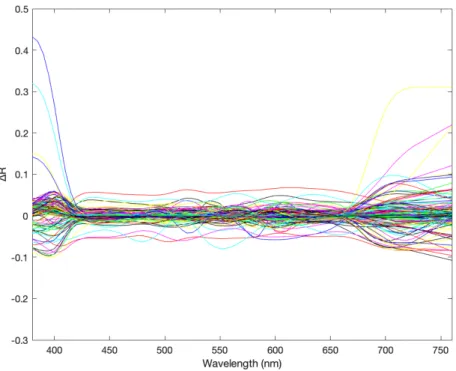
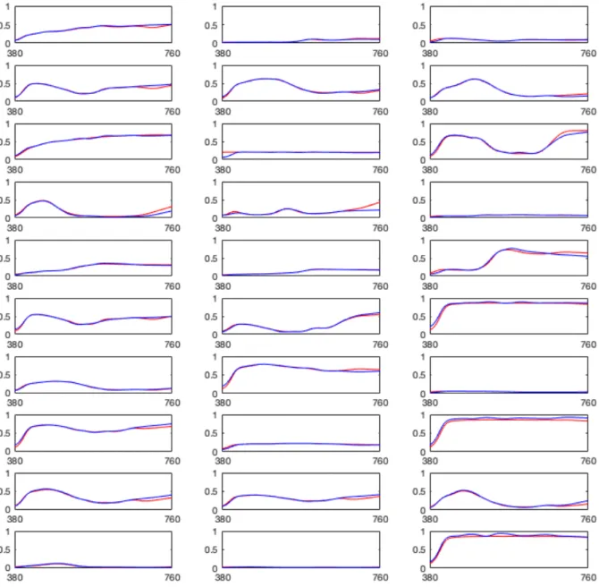
The difference in the reflectance spectra of the target and the predicted reflectance calculated from the actual camera signal and the predicted camera signal is shown in Figure 15 and Figure 16. The subplots comparing the measured reflectance from the target to the predicted reflectance calculated using the actual camera signal and the predicted camera signal is seen below (Figure 17 and Figure 18). The predicted reflectance calculated using the actual camera signal and predicted camera signal showed a good estimation with differences ranging from -0.15 to +0.45 for actual camera signal and -0.15 to +0.3 for predicted camera signal. The computed RMSE for actual camera signal is 0.03 while the RMSE for predicted camera signal is 0.02. Based on Figure 15 and Figure 16, the predicted camera signal predicted the reflectance spectra better along the visible range (400-700 nm) than the actual camera signal. However, the difference in the calculated

ΔE₀₀

(

)

(

)

(

)

(

)

RMSE is likely not significantly different from each other and both did well in predicting reflectance as seen in individual subplots of the patches in Figures 17 and 18.

The actual camera signal even after optimization (∆E00 (SL=1) of 0.89), resulted in a higher

mean color difference than the predicted camera signal ∆E00 (SL=1) of 0.15. This is expected given

that the actual imaging is affected by external factors adding noise to the actual imaging process. External factors in the imaging set up causing uncertainty in the image (e.g. environment, human and instrument error) could have affected the actual camera signal thus yielding a poorer color difference statistic.

In terms of noise, actual camera signal yields roughly similar color transformation noise as the predicted camera signal. This proves that the noise equation was able to efficiently predict the noise brought about by color transformation. This is an important result that proves the reliability of the computational imaging simulation. Computational imaging simulations sought to determine the best possible LED combination would be performed and shall be the focus in the next chapter.

The LAB vector plot for the measured and predicted colorimetric data is shown in Figure 19 and Figure 20. The predicted colorimetric data from the actual camera signal is shown in Figure 19 while the predicted colorimetric data from the calculated predicted camera signal is shown in Figure 20. The LAB vector plot for the optimized matrix cooefficients from the actual camera signal was also presented in Figure 21, since the optimized matrix coefficients from the predicted camera signal remained the same, no additional LAB vector plot was shown.

The colored dot defines the coordinates of the measured patch while the arrowhead defines the coordinates of its estimate. As seen in Figures 15-21 the camera model showed a good estimation for the reflectance and colorimetric data.

Figure 15. The difference between the measured spectra and the calculated predicted spectra from the actual camera signal.

Figure 16. The difference between the measured spectra and the calculated predicted spectra from the predicted camera signal.

Figure 17. The measured reflectance spectra (red line) compared to the predicted reflectance spectra (blue line) calculated from the actual camera signal.

Figure 18. The measured reflectance spectra (red line) compared to the predicted reflectance spectra (blue line) calculated using the predicted camera signal.

Figure 19. CIELAB a* vs. b* and L* vs. C*ab vector plots of the measured and predicted

colorimetric data calculated from the actual camera signal.

Figure 20. CIELAB a* vs. b* and L* vs. C*ab vector plots of the measured and predicted

Figure 21. CIELAB a* vs. b* and L* vs. C*ab vector plots of the measured and predicted

3.5 Conclusions

The purpose of this chapter is to verify the camera model using the currently available LEDs at Munsell Color Science laboratory. The application of LED lights in multispectral imaging is introduced. Initial experiments using the available LEDmotive system composed of 10 LEDs proved to be effective in multispectral imaging. Both metrics (RMSE and ∆E00 (SL=1) used to

evaluate spectral and colorimetric data showed high spectral and color accuracy. Noise attributed to color transformation was also reasonably low. The color transformation noise from the actual camera signal and from the predicted camera signal are roughly the same, proving the efficiency of the camera model in predicting noise brought about by color transformation. This here is vital in computational imaging simulation, as such that the behavior of the computational imaging system mimics the actual imaging system and that the camera model performed reasonably well. In addition to, the camera model was successful in predicting the camera signal with almost perfect linearity and an R2 _{of 0.99. The actual camera signal resulted in a higher mean color difference}

than the predicted camera signal. An increase in the area of the patch taken to get the actual camera signal may help in yielding a better color difference statistic. Bear in mind that the actual imaging is subjected to other types of noise. External factors in the imaging set up causing uncertainty in the image (e.g. environment, human and instrument error) could have also affected the actual camera signal.

The MATLAB fminunc optimization was able to optimize the average color difference for the actual camera signal but not significantly, perhaps another optimization method could be used to achieve the true minimum instead of the local minimum. A change in starting value could also yield a better optimization result.

All in all, this chapter proved that the camera model is valid and effective in predicting the camera signal taking into account the color transformation noise.

Chapter 4: Optimal LED Selection

This chapter describes the computational LED selection performed in order to define the optimal LED combination for a 10-channel multispectral imaging system. The chapter is divided into parts to describe the processes taken in order to narrow down the combinations and the chosen metrics used to evaluate the colorimetric and spectral accuracy of each LED combination.

4.1 LED (Light Emitting Diode) system

A total of thirty-seven lights (37) were available from LEDmotive Technologies. The manufacturer provided the normalized spectral power distribution for all 37 lights as seen in Figure 22. The lights have the wavelength range of (380 nm-760 nm). The manufacturer is able to manufacture an LED system composed of 10-12 LEDs. In order to reduce the cost, it was ultimately decided to use 10 LEDs. A straightforward method for LED selection would be to simulate all possible LED combinations and then determine the best LED combination under a given metric. Doing this is impractical, it’s computationally expensive and time consuming. Computing for all possible combinations using the permutation formula without repetition as seen in Equation 9 yields 348,330,136 combinations, where n is the combination of LEDs taken k at a time. Furthermore, since some of LEDs cluster in a specific range, it would yield uninformative combinations such as a set of all short wavelength LEDs or long wavelength LEDs. The best way to avoid this and to reduce the computational time is to group the LEDs according to their region of interest. The LEDs were divided according to a specified peak range (see Figure 1), doing this reduced the possible combinations to 110,592. The name of the LEDs is assigned as numbers 1-37 from left to right, these numbers served as the guide in identifying the optimum LED later on the experiment. LED numbers 1-9 is bin number 1, LED numbers 10-13 is bin number 2, LED numbers 14-17 is bin number 3, LED numbers 18-21 is bin number 4, LED numbers 22-25 is bin number 5, LED number 26 is bin number 6, LED numbers 27-30 is bin number 7, LED numbers 31-32 is bin number 8, LED numbers 33-34 is bin number 9 and LED numbers 35-37 is bin number 10. LED 26 is in its own bin because the LED’s peak is similar to V(λ) which is important in the spectral and colorimetric accuracy of the imaging system. Therefore, putting it in its own bin assures that the LED is chosen for all possible combinations. The LEDs with their corresponding peaks wavelength (nm) are shown in Table 4 below. In order for the imaging to be effective, the

LEDs must cover if not the entire electromagnetic spectrum then at least the range of the visible spectrum.

𝐶(𝑛, 𝑘) = 𝑛!

𝑘! (𝑛 − 𝑘)! (9)

Figure 22. Normalized spectral power distributions of 37 LEDs used in the simulation. Table 4. Peak wavelengths of the 37 available LEDs.

LED numbers Peak wavelength (nm)

1 385 2 390 3 395 4 400 5 405 6 410