Chapter 7: Methods for GIS Data Manipulation, Analysis, and Evaluation

Chapter 7: Methods for GIS

Data Manipulation,

Analysis, and

Evaluation

OVERVIEW

This chapter details the methods that the team used to 1) evaluate lands within the study area, 2) delineate Conservation Focus Areas (CFAs), and 3) prioritize individual, privately owned land parcels for protection. The chapter also describes the team’s methods for assessing and evaluating threats to the study area’s ecological integrity.

As noted previously, the project’s analysis consists of two main phases operating at two different scales.

· Phase One: Regional Scale – In this phase, the team analyzed the entire study area and ranked the matrix of lands as low, medium, high, or highest priority. The team delineated CFAs around larger clusters of high and highest priority lands.

· Phase Two: Parcel Scale – In the project’s second phase, the team analyzed privately owned parcels within the CFAs and ranked those parcels in order of their conservation importance.

For organizational and presentation purposes, this chapter describes the methods of each phase separately. It is important to note, however, that Phase Two is intrinsically linked to Phase One. In addition, the basic methodological approach for each phase is very similar. Namely, the team uses a straight-forward geographic information systems (GIS)-based analysis to spatially represent important ecological features, weight those features based on their relative ecological importance, and consolidate the individual weights to determine the relative conservation priority of landscapes and parcels within the study area. The team did not weigh threats but spatially represents as many of them as possible to depict their

relationship to the CFAs.

PHASE ONE ANALYSIS:

CFA DELINEATION AND PRIORITIZATION

There are five main steps in this phase of the analysis. Figure 7.1 summarizes the five steps of this analysis, which are described in detail in the text that follows.

Figure 7.1: Basic steps in Phase One Analysis

1. Develop conservation drivers to represent project objectives spatially. 2. Spatially represent and weight conservation drivers.

3. Use raster grids to conduct overall prioritization analysis. 4. Delineate Conservation Focus Areas (CFAs).

STEP 1: DEVELOP CONSERVATION DRIVERS

In order to incorporate the project’s goals and objectives directly into the GIS-based analysis, the team developed a tool that it termed a “conservation driver.” Simply put, a conservation driver is a spatial representation of a project objective. In most cases, the language

describing both the objective and the driver is very similar. It is important to note, however, that the two concepts are different. An objective consists of an action-oriented purpose for the project. A conservation driver is the spatial representation of that objective, a mappable entity that can be manipulated and analyzed using GIS. In other words, an objective is an idea and a driver is that idea spatially delineated on the landscape.

An example from the project helps illustrate both the close connection and the important difference between objectives and drivers. One of the project’s objectives is to Conserve Natural Areas that Exhibit a High Degree of Integrity and Resiliency. The team uses pre-settlement vegetation as the corresponding driver to measure and map intact and resilient natural areas. For every project objective, the team developed a corresponding conservation driver.1 Table 7.1 summarizes the project’s conservation drivers and their relationship to the project’s mission, goals, and objectives.

1 _{Note that some drivers support more than one objective, and that some objectives are expressed through more}

than one driver. For each objective, however, there is a primary driver that spatially expresses the objective more directly and effectively than others.

Table 7.1: Mission, Goals, Objectives, and Conservation Drivers

Mission: To guide future work and investment of the Grand Traverse Regional Land Conservancy in the Manistee River watershed, this project will identify areas of high conservation value and, within those areas, prioritize privately owned land parcels for protection efforts.

Goals Objectives Conservation Drivers

Protect hydrologic integrity of the

upper Manistee River watershed Groundwater accumulation

Conserve wetland ecosystems Wetlands

Conserve riparian ecosystems Riparian ecosystems

Maintain biodiversity Element occurrences

Protect a diversity of local ecosystems Rare landtype associations

Conserve Areas of High Ecological Importance

Conserve natural areas that exhibit a

high degree of integrity and resiliency Pre-settlement vegetation Conserve unfragmented landscapes Large tracts ofunfragmented natural areas Promote the expansion and integrity of

existing protected areas Expansion and integrity ofexisting protected lands

Promote Spatial Integrity of the Landscape

Target large land parcels Parcel size*

Identify and Delineate Threats to Ecological Systems and Processes

Analyze threats and their sources and,

when possible, map those sources Sources of threats**Ø Development Ø Oil and Gas Drilling Ø Incompatible Logging Ø Invasive Species

Ø Road Development

Ø Off-Road Vehicle Use Ø Fire Suppression

Ø Dams

*Not a weighted conservation driver but used in parcel analysis and prioritization. **Not weighted or used on CFA or parcel prioritization.

STEP 2: SPATIALLY REPRESENT & WEIGHT CONSERVATION

DRIVERS

As the second step toward prioritizing lands within the study area for protection, the team spatially represented each driver and assigned weights to each driver according to its relative conservation value. The team conducted these activities using geographic information systems (GIS).

The wetlands driver provides a simple example of how the team used conservation drivers to help prioritize lands within the study area. For this driver, the team analyzed GIS data that

depicted the location and extent of wetlands within the study area. The team assigned a weight of 10 points to those areas that contained wetlands and 0 points to all other lands in the study area. Table 7.2 summarizes the basic analysis and associated weights the team used for each conservation driver.

Table 7.2: Basic analysis and weighting scheme for the conservation drivers Conservation

Driver

Basic Analysis Weighting Scheme

Groundwater

Accumulation Examined groundwater accumulationdata and classified areas according to standard deviation (SD) from

statewide mean.

· Areas with accumulation levels greater than or equal to 2 SD: 10 points

· Areas with accumulation levels <2 and > 1 SD: 5 points

· All other areas: 0 points

Wetlands Analyzed as present or absent. · Wetlands: 10 points

· Non-Wetlands: 0 points

Riparian Ecosystems

Used two different buffer distances to

prioritize riparian areas. ·

Lands within 50m of all streams and lakes: 10 points

· Lands between 50 and 300m of river's mainstem: 5 points

· Lands outside those buffers: 0 points

Element

Occurrences Calculated point density of elementoccurrences and reclassified results using standard deviation (SD) from mean.

· Areas with occurrence density > 2 SD: 10 points

· Areas with occurrence density between < 2 and > 0 SD: 5 points

· Areas with occurrence density less than or equal to 0 SD: 0 points

Rare Landtype

Associations Analyzed according to two thresholds:the overall rarity of LTA within the ecoregion and the percentage of that rarity contained within the study area.

· LTAs passing both rarity and study area representation thresholds: 10 points

· LTAs passing only one threshold: 5 points

· All other LTAs: 0 points

Pre-settlement Vegetation

Analyzed the overlap between estimated 1800 land cover and present day land cover and examined areas exhibiting cover resembling pre-settlement vegetation.

· Highest priority areas of overlap: 10 points

· High priority areas of overlap: 5 points

· All other areas: 0 points

Large Tracts of Unfragmented Natural Areas

Examined contiguous natural areas (not bisected by main roads) and analyzed them according to relative size and distance of centroid from nearest road.

· Areas > or equal to 1,000 acres and centroid is > or equal to 500m from roads: 10 points

· Areas > or equal to 1,000 acres and centroid is < 500m from roads: 5 points

· All other areas: 0 points

Expansion and Integrity of Existing Protected Lands

Used two different buffers – expansion and integrity – to prioritize private lands within the study area.

· Lands within the integrity buffer and 880 m or less from protected lands:

10 points

· Lands within expansion buffer or within the integrity buffer but > 880 m from protected areas: 5 points

While Table 7.2 provides an overview of the conservation drivers used in the Phase One analysis, understanding their individual roles and impacts in the overall project requires a more thorough examination. The following portion of this section describes the justification, approach, and manipulation of each driver in detail.

Groundwater Accumulation Driver Justification

The team used groundwater accumulation areas as a spatial representation of its objective to conserve the hydrological integrity of the upper Manistee River watershed. While there are several possible landscape features one could prioritize in an effort to preserve hydrologic integrity (surface waters, intact forestland, etc.), the team felt that no feature was as important to the Manistee River system as lands that support high levels of groundwater accumulation. While the importance of groundwater in cold-water or cool-water rivers is well documented, there has been some uncertainty over which lands within a watershed are the most critical for the protection of groundwater integrity. Over the last few decades, ecologists and

hydrologists have struggled to provide quantifiable answers to this question. In large part, their work has involved modeling efforts at the local and regional scales that attempt to predict the connections between groundwater inputs and surface water features. However, few of these models have been successful at making accurate predictions at a scale that is useful to resource managers (Baker, et al., 2001). Most earlier efforts used very localized data - such as well logs that document water table depth – to drive their models.

Reproducing these at the regional scale is extremely data intensive and time consuming. The recent work of Matt Baker, Dr. Mike Wiley, and Dr. Paul Seelbach at the University of Michigan’s School of Natural Resources and Environment has demonstrated significant potential in overcoming these scale-related problems. One of the models they have produced, the MRI-DARCY[IO] V.3 (also called the Darcy input/output model), seems especially strong and appropriate for the Upper Manistee Project. The raster-based model uses a digital elevation model (DEM) and a surficial geology map in a GIS-application of Darcy’s Law to map the potential relevance of groundwater to surface water interactions for the state of Michigan (Baker, et al., 2001). Darcy’s Law states that the velocity of flow through a porous medium is proportional to the difference in hydraulic head over some flow-path length (hydraulic slope) and the hydraulic conductivity of the medium (Baker, et al., 2001).2 For example, velocity will increase as slope increases and conductivity remains constant. Based on this equation, the input-output model maps areas with the potential for groundwater accumulation (inflow) and groundwater recharge (outflow).

While both accumulation and recharge areas are important to protect, the team decided to focus on potential accumulation areas only. The reasons for the decision are as follows:

2 _{Darcy’s Law states that q = kiA, where q = flow rate, k = hydralic conductivity, i = the change in head over a}

· The upper Manistee region is dominated by sandy soils, so virtually all lands

contribute to groundwater recharge. Therefore, weighing groundwater recharge areas is not selective and would not help prioritize areas for protection.

· Groundwater recharge is less understood and more difficult to define geographically than groundwater accumulation (Baker, et al., 2001).

· Groundwater transport may not be defined by watershed boundaries. In other words, some of the groundwater that eventually surfaces in the Manistee River may have originated outside the study area and is thus outside the scope of this project. · Groundwater accumulation areas are especially vulnerable to contamination due to

shallow water table depths.

· Groundwater accumulation areas play a critical role in the Manistee’s hydrological and biological characteristics.

It is important to understand the basic characteristics of lands that the MRI-DARCY[IO] v.3 identifies as groundwater accumulation areas. In a raster-based analysis, groundwater

accumulation occurs when numerous grid cells with high rates of groundwater transport drain into grid cells that have lower transport values based on differences in slope or surficial geology. The resulting build-up of groundwater can produce either an upwelling in the form of cold groundwater springs or a groundwater table that is at or near the surface. Protecting these areas is critical to the conservation of the Manistee River system primarily because development on these lands can produce the following hydrologic impacts:

· Development increases impervious surfaces, which, in turn, increase runoff of warmer water into the river system.

· Development often leads to an increase in chemical and fertilizer use, both of which can runoff into nearby surface waters or seep into the shallow groundwater aquifer.

· Development can reduce the landscape’s hydrological connectivity, which can disrupt the routing of hydrologic inputs into the river system.

The MRI-DARCY[IO] v.3 model does not take into account surface water features. Therefore, groundwater accumulation areas that the model identifies may actually be

groundwater-fed wetlands or lakes. While this may seem somewhat duplicative of the team’s riparian and wetland drivers, the MRI-DARCY[IO] v.3 model allows the team to

differentiate and give higher scores to those wetlands, riparian lands, and other areas that contribute significantly higher amounts of cold groundwater into the stream system. Approach

transport occurs at the particular location. The actual data can be displayed and used in a variety of ways. The most useful is to classify the raster cells using standard deviation. Using standard deviation allows the user to compare a cell’s variability from the mean value. This positive or negative deviation from the mean can then be translated into groundwater accumulation areas or groundwater recharge areas respectively (Figure 7.2).

Figure 7.2: MRI – DARCY[IO] v. 3 classified using the standard deviation thresholds at the state level 0 10 20 30 Kilometers N MRI - DARCY[IO] v.3 Standard Deviation <-3 std. dev. -2.00 -1.00 mean 1.00 2.00 >3 std. dev.

Source: Michigan Rivers Inventory

Classifying the data in relation to the state average illustrates how the watershed as a whole compares to the rest of the state. In summary, the Manistee watershed exhibits a high level of groundwater recharge and has a number of important groundwater accumulation areas. This comparison ultimately helps identify those accumulation areas that are most significant across the study area.

The team used two threshold values to assign weights. Areas with groundwater

accumulation levels greater than or equal to 2.00 standard deviation from the mean received 10 points. Areas that had accumulation levels between 1.00 and 2.00 standard deviation from the mean received 5 points. All other areas received 0 points. The team selected these thresholds based on the use of standard deviation in statistical literature.

Data Sources

Table 7.3: Data used for analysis of groundwater accumulation driver Dataset Year

Published

Format Scale Originator & Source Original Projection MRI-DARCY[IO] v.3 Groundwater Model 2001 Digital raster

data ModelDEM 1:24,000

Geology 1:250,000 Baker, et al. Michigan Rivers Inventory UTM, NAD 83, zone 16 Data Manipulation

The team performed the following basic manipulations on the GIS data. 1. Calculated the mean transport value for the entire state of Michigan.

2. Clipped the MRI-DARCY[IO] v.3 model to the study area boundary, making sure to preserve the standard deviation values at statewide levels.

3. Reclassified the MRI-DARCY[IO] v.3 model by assigning a score of 0, 5, or 10 points to every grid cell depending on its standard deviation values.

4. Converted the reclassified MRI-DARCY[IO] v.3 model to a shapefile.

5. Reprojected the DARCIO data into Michigan Georef so that it could be combined with the other drivers’ data layers.

6. Transformed the shapefile back into a grid with 30-meter grid cells to allow priority values to be added between the various drivers.

Wetlands Driver Justification

The wetlands conservation driver serves as a direct spatial representation of the project’s objective to conserve wetland ecosystems. As such, it is one of the project’s most

straightforward conservation drivers and requires relatively little computational analysis and data manipulation to translate it from an objective to discrete features on the landscape. The wetlands driver also addresses the project’s objective of maintaining the study area’s

hydrologic integrity and biodiversity. Approach

The study area contains a variety of wetland types and sizes. There are at least eight different kinds of wetlands when they are classified according to dominant vegetation and even more types when factors such as soil and water chemistry are considered. In addition, the study

area contains wetlands of various sizes, ranging from several hundred acre complexes to small, vernal pools. Despite the unique characteristics of the wetlands in the study area, the wetlands driver does not differentiate between types or sizes for two main reasons. First, taking a similar approach to a past Master’s project at the School of Natural Resources and Environment, the team concluded that different wetlands provide different functions and that conserving a diversity of wetland ecosystems is, in itself, important (Brammeier et al., 1998). Second, the existing GIS data is generally more reliable for depicting wetland locations than it is in capturing the specific attributes of individual wetlands. To treat all wetlands equally, the team simply analyzed the study area for presence or absence of wetlands. All wetland areas received 10 points and all non-wetland areas received 0 points.

Data Sources

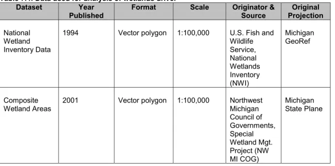
The project team used two different sources of wetland data. The Northwest Council of Governments (NW MI COG) created composite wetland coverages for Kalkaska, Antrim, and Missaukee counties using data from the U.S. Fish and Wildlife Service’s National Wetlands Inventory (NWI), soils maps from the Natural Resources Conservation Service, and land cover data from the Michigan Resource Inventory System. Field investigations by GTRLC and others have revealed that this composite data is generally more thorough and more accurate than using NWI data alone. Unfortunately, composite data is not available for Otsego and Crawford counties. For these localities, the team used the NWI data, the best data publicly available. Table 7.4 summarizes and describes the primary data used for this driver.

Table 7.4: Data used for analysis of wetlands driver Dataset Year

Published Format Scale Originator &Source ProjectionOriginal

National Wetland Inventory Data

1994 Vector polygon 1:100,000 U.S. Fish and

Wildlife Service, National Wetlands Inventory (NWI) Michigan GeoRef Composite

Wetland Areas 2001 Vector polygon 1:100,000 NorthwestMichigan

Council of Governments, Special Wetland Mgt. Project (NW MI COG) Michigan State Plane

Data Manipulation

The team performed the following basic manipulations on the GIS data.

1. Reprojected the NW MI COG composite wetland data from Michigan State Plane to Michigan GeoRef using an extension from the Michigan DNR Spatial Data Library and the Reprojection Wizard on ArcView.

2. Merged the NWI data and the NW MI COG data and clipped the merged layer to the study area boundary.

3. Selected all wetland areas from the attribute table and assigned them a score of 10. All other areas were scored 0.

4. Converted the combined wetland shapefile to a grid based on weights in the attribute table.

Riparian Ecosystems Driver Justification

Similar to the extremely close association between the wetlands objective and wetlands driver, the riparian ecosystems conservation driver serves as a direct spatial representation of the project’s objective to conserve riparian ecosystems. The only real analysis and data manipulation necessary to translate the objective into discrete landscape features was selecting and delineating the spatial boundaries for the riparian ecosystems. Also, like the wetlands driver, the riparian ecosystem driver secondarily addresses the project’s objective of preserving the hydrologic integrity and maintaining biodiversity in the study area.

Approach

The team considered two possible ways to select and delineate riparian ecosystems. The first approach (which the team initially preferred but did not select) was to delineate a boundary separating the river floodplain from adjacent non-riverine uplands using remotely sensed images. The team hoped to map and highlight dynamic river floodplain ecosystems, rather than simply applying a static buffer distance to the entire stream network. This approach would have produced riparian buffers of varying widths because the breadth of the riparian zone fluctuates along the stream course (Budd, et al, 1987). Baker, et al. (1998) successfully used color infrared aerial photographs to delineate and highlight the diversity of landscape ecosystem at a fairly large scale in the Manistee river floodplain. Although the team had hoped to perform a simple analysis at a far smaller scale to make it useful for its work, the process ultimately proved to be beyond the scope of the project.3

3 _{Although beyond the scope of this project, delineating riparian ecosystems based on actual floodplain}

As an alternative, the team decided to delineate riparian ecosystems by using two different buffer distances to surround streams and lakes. First, the team created a 50-meter buffer around all riparian features, regardless of size. Lands within this buffer received 10 points. Additionally, the team created a second buffer of 51-300 meters around the main stem of the Manistee River. Lands within this buffer received 5 points. Figure 7.3 below displays the general buffering approach.

Figure 7.3: Buffers created to represent the riparian corridor

0 1 2 3 Kilometers Score* 0 Points 5 Points 10 Points Lakes Streams N Main Branch Manistee River Tributaries

* Lands within 50m of all streams and lakes - 10 points; Lands between 50 and 300m of river's mainstem - 5 points; Lands outside those buffers - 0 points

The team chose these buffer distances based on a visual inspection of floodplain widths in Digital Orthophotoquads of the study area. Fifty meters exceeded the average floodplain width, and 300 meters exceeded the width of the widest sections of the floodplain within the study area.

Scientific findings help justify the project team’s selection of two differentially sized and scored buffer distances. Karr and Schlosser (1978) stress the importance of maintaining near-stream vegetation; therefore, it is logical to place a high conservation emphasis on preserving the lands closest to all water bodies (in this case, those lands within 50 meters). Lands that lie farther away from surface waters do influence the health of aquatic ecosystems

streams using color infrared aerial photographs in combination with topographic maps or, preferably, digital elevation models.

and are therefore also important to this driver. The team chose to place this second buffer distance around only the mainstem of the Manistee River because, in general, buffer

effectiveness decreases with increasing stream size (Karr and Schlosser, 1978). In first and second order streams (headwaters and tributaries), buffers are extremely effective and do not need to be very wide in order to have a positive impact on aquatic systems. With larger streams, however, relatively narrow buffers tend to have less of a positive impact on the associated health of the aquatic ecosystems. Thus, the larger the stream, the larger the buffer required to mitigate the effects of nutrient loading, sedimentation, and erosion.

The specific buffer widths of 50 and 300 meters are more than adequate when compared with most management recommendations. In the Pacific Northwest, for example, researchers determined that corridors of riparian vegetation 11 to 38 meters wide on both sides of stream provide favorable habitat conditions for salmon (Ahern, 1991). With regard to lakes, the literature recommends preserving a natural buffer zone of at least 15 meters from the

shoreline (Henderson, et al., 1998). Other researchers suggest that buffers of 31 to 61 meters will generally maintain ecological health (Budd, et al., 1987). The project team’s riparian buffers clearly exceed the distances recommended for sustaining ecological health, thereby helping to ensure maximum protection for riparian ecosystems within the study area. Data Sources

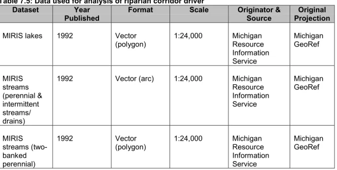
The team identified three possible sources for hydrologic data through MDNR Spatial Data Library: MIRIS, Census Data, and USGS Digital Line Graph. The team selected the MIRIS data because it was created at the smallest scale – 1:24,000. The other sources were created at a scale of 1:100,000. Table 7.5 summarizes and describes the primary data used for this driver.

Table 7.5: Data used for analysis of riparian corridor driver Dataset Year

Published Format Scale Originator &Source ProjectionOriginal

MIRIS lakes 1992 Vector

(polygon) 1:24,000 Michigan Resource Information Service Michigan GeoRef MIRIS streams (perennial & intermittent streams/ drains)

1992 Vector (arc) 1:24,000 Michigan

Resource Information Service Michigan GeoRef MIRIS streams (two-banked perennial) 1992 Vector

(polygon) 1:24,000 MichiganResource

Information Service

Michigan GeoRef

Data Manipulation

The team performed the following basic manipulations on the GIS data. 1. Clipped each hydrology layer to the study area.

2. Created a 50 meter buffer around all streams and lakes.

3. Created a 51-300 meter buffer around the polygon stream layer that consisted solely of the mainstem of the Manistee River in the study area.

4. Performed a union of the buffer layers (0-50 meters and 51-300 meters) to create one final buffer file.

5. Added a column to the attribute table and entered appropriate scores – 10 points for the 0-50 meter buffer, and 5 points for the 51-300 meter buffer.

6. Converted the layer to a 30 meter raster grid.

Element Occurrences Driver Justification

This project seeks to produce an ecosystem-based conservation plan that prioritizes lands based on their capacity to preserve a host of ecological features and functions, rather than the management or habitat requirements of a few targeted species. At the same time, however, the project team recognizes that threatened and endangered species represent an important conservation consideration and that biota is a very important ecosystem component. For these reasons, the team decided to incorporate species information into the overall analysis by prioritizing areas for conservation based on the relative density of element occurrences (rare plants, animals, or communities) throughout the study area. This driver links directly to the project’s objective of maintaining biological diversity.

Approach

In structuring our analysis, the project team chose to use point data to calculate the density of element occurrences. There were two main factors in this decision.

· First, since this project focuses on the general protection of biodiversity rather than the conservation of specific species, the team felt it was more appropriate to score areas based on the density of element occurrences rather than the presence of any one

individual species. Implicit in this approach is the notion that all elements are of equal importance, regardless of species, specific protection status, or rank. The team wanted to avoid making largely arbitrary decisions regarding the relative conservation value of individual elements and calculating occurrence density was, therefore, a logical approach.

· Second, because data collection methods and associated spatial accuracy varied

throughout the data set, the team felt it was more appropriate to look for general trends across the landscape than it was to try to determine exact spatial extent of occurrences. Data Sources

There are three main categories of element occurrences in the study area: animals, plants, and natural communities. The natural communities are based on vegetation and habitat types. All animal and plant element occurrences have some level of state protective status.

Communities are not listed on either the state or federal level but are included by Michigan Natural Features Inventory (MNFI) in the element occurrence database because they are rare globally and/or within the state or possess some other unique features meriting protection. There are a total of 56 elements occurrences in the study area, representing nine different animals, eight different plants, and five different communities. Please see Appendix A for more information.

MNFI provides the element occurrence data as both polygon and point coverages. According to Edward Schools, a Program Leader for Conservation and GIS at MNFI, MNFI generated the polygon coverage using two basic methods. If MNFI collected the data before it

integrated GIS with its field surveys, the element occurrence was assigned a buffer, the extent of which depended on the degree of spatial accuracy of the record. The greater the spatial accuracy, the smaller the buffer. If MNFI collected the data after integration with GIS, the element occurrence was digitized based on its known spatial extent. The point data represent the centroid of the polygons. While the spatial accuracy of the points is limited (i.e. the location of any one point does not guarantee the presence of an occurrence at that point on the ground), the point data is suitable for determining the overall density of

occurrences (Schools, October 2002). Table 7.6 summarizes and describes the primary data used for this driver.

Table 7.6: Data used for analysis of element occurrence driver Dataset Year

Published Format Scale Originator &Source ProjectionOriginal

Biotic (Point)

Database 2001 Vector (point) N/A RebeccaBohem,

Michigan Natural Features Inventory Michigan GeoRef Data Manipulation

The team performed the following basic manipulations on the GIS data. 1. Clipped MNFI point data to the study area boundary.

2. Per advice from other conservation planners, edited the attribute table to remove seven records that were older than 1986 in an attempt to minimize errors resulting from historic data (The Nature Conservancy of Colorado, 2001).

3. Determined density of element occurrences within the study area by using Calculate Density function in ArcView. Set the output grid extent equal to the study area boundary and selected a one square kilometer grid size and a 2,000 meter search radius. Set the density to calculate as a kernel density and selected output grid units as square

kilometers.

4. The resulting grid displayed values for density of element occurrences per square kilometer.

5. Since the raw scores for overall density were relatively low and difficult to distinguish from each other in meaningful ways, reclassified the raw scores using standard deviation (SD), with breaks at 1 SD. This reclassification illustrated statistical patterns in the original scores and allowed for reasonable assignment of weighted scores for the driver (Table 7.7).

Table 7.7: Reclassification and weighting calculations for element occurrence driver Original Density Reclassification Weights

-0.056 to 0.015 <-1 to 0 SD 0 0.016 Mean 0 0.017 – 0.087 >0 – 1 SD 5 0.088 – 0.159 >1 – 2 SD 5 0.160 – 0.231 >2 – 3 SD 10 0.232 – 1.442 >3 SD 10

6. Converted the resulting grid to a shapefile and assigned weights based on the SD reclassification scheme.

7. Lastly, converted the scored shapefile back to a grid using 30 meter grid cells so that data for this driver could be combined with other grids.

Rare Landtype Associations Driver Justification

To represent the objective of protecting a diversity of local ecosystems spatially, the team used landtype associations (LTAs) as the foundation for this conservation driver. LTAs are relatively large-scale local ecosystems that MNFI delineated primarily based on

physiography and soils and secondarily on vegetation (see Chapter 5) (Albert, 1995 and Corner, 1999). LTAs are ecosystem types, any one of which can occur in multiple locations. The study area consists of more than 20 LTAs, with 17 different LTA types. Ideally, the

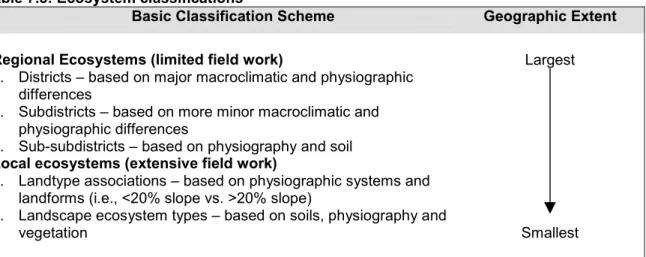
team would incorporate information from the landscape ecosystem type level (the smallest-scaled ecosystem unit), but LTAs represent the finest scale delineation for which data is currently available within the study area. See Table 7.8 for more information on how LTAs fit into the larger ecosystem classification scheme.

Table 7.8: Ecosystem classifications

Basic Classification Scheme Geographic Extent Regional Ecosystems (limited field work)

1. Districts – based on major macroclimatic and physiographic differences

2. Subdistricts – based on more minor macroclimatic and physiographic differences

3. Sub-subdistricts – based on physiography and soil

Local ecosystems (extensive field work)

1. Landtype associations – based on physiographic systems and landforms (i.e., <20% slope vs. >20% slope)

2. Landscape ecosystem types – based on soils, physiography and vegetation

Largest

Smallest

The team gives priority to rare LTAs within the study area in order to highlight the importance of protecting a diversity of landscape ecosystems. Secondarily, protecting a diversity of ecosystems helps the team achieve its objective of maintaining biodiversity. Approach

To determine the relative rarity of the different LTAs, the team used the nested hierarchy outlined in Table 7.8 and examined LTAs against the next level of ecosystems in that

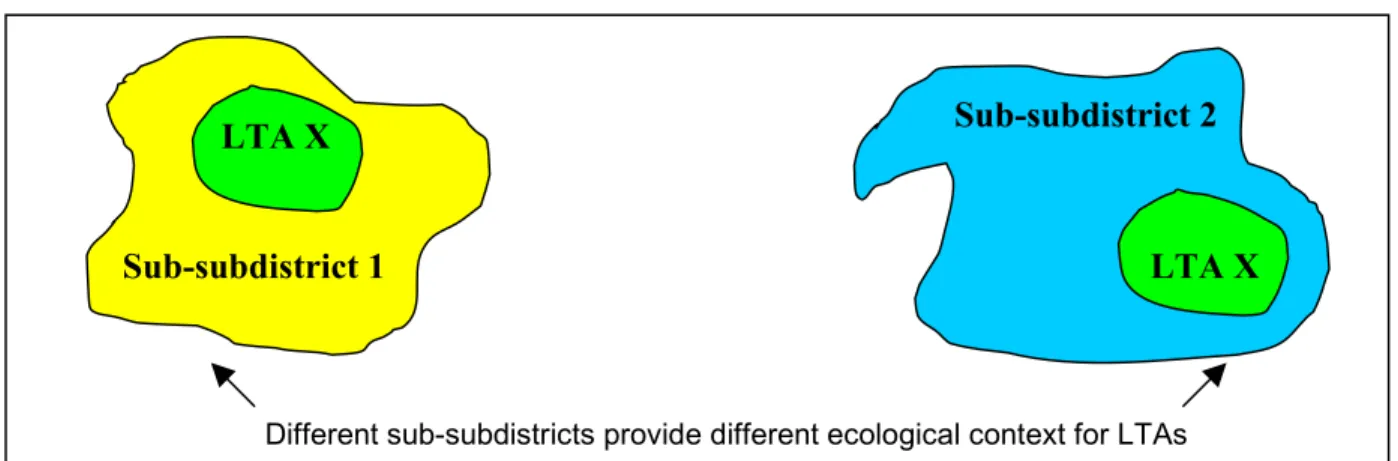
hierarchy – the sub-subdistricts. The team made this decision understanding that the various levels of ecosystem classification have ecological, as well as organizational, significance. In other words, the hierarchy helps outline the full extent of ecosystem diversity and helps clarify the importance of protecting local ecosystems. Figure 7.4 helps illustrate this point. In this figure, there are two identical (by description) LTAs, both labeled LTA X. Each LTA X, however, is nested within a different sub-subdistrict. Therefore, while their descriptions may be identical, the ecological context of the landscapes surrounding each LTA X is different. By extension, the relative conservation value of each LTA X may also be quite different.

The study area includes portions of two sub-subdistricts – Grayling Outwash Plain and Cadillac. Grayling Outwash Plain covers over 98 percent of the study area, while Cadillac only contains a small portion of the study area’s southern corner. The team calculated the conservation value of LTAs in both sub-subdistricts using two specific criteria – overall rarity and study area representation.

· Overall Rarity – To determine overall rarity, the team calculated the percentage of each sub-subdistrict covered by each LTA within the study area. The smaller the percentage, the more rare the team judged the individual LTAs on a regional scale.

· Study Area Representation – The team then calculated what percentage of each LTA within the entire sub-subdistrict was found in the study area. In this case, the team assigned priority to LTAs with higher percentages. For example, if 100% of the sub-subdistrict’s LTA was found in the study area, protection of that LTA became a higher priority because it is found nowhere else in the sub-subdistrict regional ecosystem unit.

Figure 7.4: Illustration of the contextual differences between two “identical” LTAs.

After selecting these two criteria, the team then established two thresholds to help determine the final weighting considerations (see Appendix B for additional detail on the analysis of the rare landtype association driver):

· Overall Rarity Threshold – The LTA represents less than one percent (<1%) of the total land area of the sub-subdistrict.

· Study Area Representation Threshold – More than 70 percent (>70%) of the land area of the LTA in the sub-subdistrict is found within the study area.

If an LTA passed both thresholds, the team awarded it 10 points. If an LTA passed only one threshold, the team awarded it 5 points. All other LTAs received 0 points.

Note that the team analyzed LTAs within both sub-subdistricts but found that no LTAs within Cadillac represented conservation priorities according to the two criteria described above. Therefore, all LTAs designated as rare and given points for prioritization purposes are found within Grayling Outwash Plain.

Data Sources

In 1999, ecologists Corner and Albert and GIS technicians Austin and DeLain completed the Landtype Associations of Northern Michigan Section VII, and the Michigan Natural Features Inventory published the dataset. The delineation of LTAs furthers the work of Barnes,

Different sub-subdistricts provide different ecological context for LTAs

LTA X

LTA X Sub-subdistrict 1

Albert, and others in mapping ecosystems from a regional to a local level. Table 7.9 summarizes and describes the primary data used for this driver.

Table 7.9: Data used for analysis of rare LTA driver Dataset Year

Published Format Scale Originator &Source ProjectionOriginal

Landtype Associations of Northern Michigan Section VII 1999 Vector

(polygon) 1:63,360 Albert, Michiganet al.; Natural Features Inventory Michigan GeoRef Ecoreg100 – Regional Landscape Ecosystems of Michigan 1995 Vector

(polygon) 1:500,000 Albert; MichiganNatural Features Inventory

Michigan GeoRef

Data Manipulation

The team performed the following basic manipulations on the GIS data.

1. To calculate the rarity of the LTA in the sub-subdistricts, clipped the LTA coverage to the boundary of Grayling Outwash Plain and Cadillac, and then determined the area of each LTA within that boundary as compared to the overall area of the sub-subdistrict. 2. To calculate the importance of the study area to the overall occurrence of the LTA in the

sub-subdistrict, clipped the LTA coverage to the study area boundary. Calculated the area of each LTA in the study area and compared those areas to the total amount of the LTA within the entire sub-subdistrict.

3. Calculated weights using the two thresholds. LTAs that passed both thresholds were awarded 10 points. LTAs that passed one threshold were awarded 5 points. LTAs that passed neither threshold were awarded 0 points.

4. Added weights to a new column in the attribute table and scored LTAs accordingly. 5. Converted the shapefile to a grid based on those weights.

Pre-settlement Vegetation Driver Justification

The pre-settlement vegetation conservation driver translates the project’s objective of conserving natural areas that exhibit a high degree of ecological integrity and resiliency into

measurable and mappable units on the landscape. Ultimately the team hoped to develop direct, quantitative measures for ecological integrity and resiliency for the full diversity of local ecosystems found in the study area. However, measuring all those factors across a large landscape is extremely data intensive and would require extensive fieldwork that is beyond the scope of this project. Alternatively, the project team recognizes that certain vegetative covers can serve as a proxy for more complex measurements of ecological integrity. If the vegetative composition and structure of an area resembles that of

pre-settlement conditions, it likely indicates that other ecological processes are intact and that the area has maintained many of its historic structural and functional components. Therefore, it is likely that the area contributes to the ecological integrity of the larger landscape.

For example, extant jack pine forests have likely maintained some degree of their historic fire disturbance regime because fire is necessary to regenerate jack pine seedlings and produce a variable forest structure. In turn, the healthy jack pine forests are likely to support and sustain a fairly high measure of their historic diversity of flora and fauna that have naturally occurred over time. The Kirkland’s Warbler, a federally listed endangered species, still thrives in jack pine forests where disturbance regimes have been maintained. Areas with vegetative cover resembling pre-settlement conditions have also proven to be more resilient to invasions by non-native species and other foreign disturbances that can jeopardize ecological integrity (Landres et al., 1999).

Approach

The pre-settlement vegetation analysis attempts to identify those lands within the study area that possess vegetative communities that resemble the communities that existed before European settlement. Essentially, the analysis compares two different land cover

classifications. The first classification approximates vegetative conditions in the early to mid-1800s (pre-settlement vegetation), and the second classifies vegetative cover based on 1978 data.

The two data sets were developed using separate and differing classification systems based upon the objectives of the original studies. The pre-settlement data contains classes that have very specific definitions based upon vegetative conditions. The 1978 land cover data

contains several classes that correspond to the increased human use of the landscape and has more generalized vegetation classes. To compare these two data sets, the team reclassified the pre-settlement features to the more generalized 1978 vegetation classes. Reclassification of the pre-settlement data was completed by analyzing the Anderson Level III and IV

classification codes used in both the pre-settlement classification scheme and the 1978 data and then regrouping the pre-settlement data using the team’s knowledge of ecosystems and plant communities of Michigan (Appendix C). Table 7.10 provides a simplified version of how the team reclassified the land cover categories.

Based on the reclassified land cover types, the team spatially compared the reclassified pre-settlement data to the 1978 land cover data. The team identified areas of overlap between the two categories as lands that presently support vegetative cover resembling pre-settlement conditions.

The team differentially scored the areas resembling pre-settlement vegetation by comparing each area to 1992 Digital Orthophotoquads obtained from MDNR. The team assessed each pre-settlement category and awarded each area of overlap either five or ten points, based upon its confidence in how the results compared to the visual inspection of aerial

photographs and the overall level of generalization made during the reclassification. For example, the team reclassified the pre-settlement “Beech-Sugar Maple-Hemlock Forest” into the 1978 “central hardwood” classification, which includes sugar and red maple, beech, basswood, cherry, and ash. Inspection of aerial photos revealed that many areas classified as central hardwood in the 1978 data set also contained various patches of aspen, indicating possible errors and generalizations in the 1978 classification or land cover changes that had occurred since 1978. In this case the team awarded “central hardwood” areas five points, expressing our lower confidence in this pre-settlement comparison. Please see Table 7.10 on the following page for more detail on point assignments for overlapping land cover

classification. Data Sources

MNFI biologists derived pre-settlement conditions by analyzing detailed notes that were taken by surveyors from the General Land Office between 1816 and 1856. The surveyors took these notes during the first Public Land Survey that divided the State of Michigan into townships and sections. Surveyors documented the location, species, and diameter of every tree used to mark section lines and corners. In addition, the notes included information on the location of rivers, lakes, wetlands; the agricultural potential of the soils; and timber quality. Potential errors in the notes and MNFI’s interpretation of vegetative conditions contribute to errors in this analysis.

For the 1978 land cover/land use classification, the Michigan Department of Natural

Resources and Michigan State University compiled data from county and regional planning commissions or their subcontractors and then converted that data into a GIS layer. Table 7.11 summarizes and describes the primary data used for this driver.

Table 7.11: Data used for analysis of pre-settlement vegetation driver Dataset Year

Published Format Scale Originator &Source ProjectionOriginal

MIRIS Land Use/Land Cover 1978 1999 Vector (polygons) 1:24,000 Michigan Dept. of Natural Resources Michigan GeoRef Land Use

circa 1800 2000 Vector(polygons) 1:24,000 MI NaturalFeatures

Inventory Michigan GeoRef 1992 Series USGS Digital Orthophoto Quadrangles 2001

Remote-sensing image 1:24,000 MDNR,Resource

Mapping and Aerial Photos

Michigan GeoRef

Table 7.10: Reclassification of pre-settlement and 1978 land cover data 1978 Land Cover

Categories Pre-settlement LandCover Categories Pre-SettlementComparison Categories

Weights

Aspen Aspen-Birch Forest Aspen 10

Aspen, Birch Aspen-Birch Forest

Undifferentiated

Aspen/White Birch Aspen-Birch

Aspen, Birch 10

Black Spruce Muskeg/Bog Black Spruce 10

Cedar Cedar Swamp, Mixed Conifer

Swamp Cedar 10

Central Hardwood Beech-Sugar Maple-Hemlock Forest Central Hardwood 5

Emergent Wetland Shrub Swamp/Emergent Marsh Emergent Wetland 10

Herbaceous Rangeland Grassland Herbaceous

Rangeland

5

Jack Pine Pine Barrens, Jack Pine-Red Pine Jack Pine 5

Lowland Conifer Cedar Swamp, Mixed Conifer

Swamp Undifferentiated

Lowland Conifer Cedar Swamp, Mixed ConiferSwamp

Lowland Conifer 10

Lowland Hardwood Black Ash Swamp, Mixed Hardwood

Swamp LowlandHardwood 10

Northern Hardwood Beech-Sugar Maple-Hemlock Forest

Undifferentiated Northern Hardwood

Beech-Sugar Maple-Hemlock Forest

Northern Hardwood

5 Other Upland Conifer Hemlock, Hemlock-White Pine,

Sugar Maple, Hemlock-Yellow-birch

Other Upland

Conifer 10

Pine White Pine, Jack Pine, Red

Pine-Jack Pine, Red Pine-White Pine, White White Oak, Red Pine-Oak, White Pine-Beech-Maple Undifferentiated Pine Oak, White Pine, Red

Pine-Jack Pine, Red Pine-White Pine, White Pine-White Oak

Pine 5

Red Oak White Pine-Mixed Hardwood Red Oak 5

Shrub Rangeland Herbaceous-Upland Grassland,

Oak-Pine Barrens

Shrub Rangeland 10

Shrub/Scrub Wetland Shrub Swamp/Emergent Marsh Shrub/Scrub

Wetland 10

Sugar Maple Beech-Sugar Maple-Hemlock Forest Sugar Maple 5

Tamarack Muskeg/Bog Tamarack 10

White Pine White Pine-Mixed Hardwood Forest,

White Pine-Red Pine Forest, White Pine-White Oak Forest

White Pine 10

Wooded Wetland Black Ash Swamp, Cedar Swamp,

Mixed Conifer Swamp, Mixed Hardwood Swamp

Data Manipulation

The team performed the following basic manipulations on the GIS data:

1. Clipped both the “MIRIS Land Use/Land Cover 1978” and “Land Use circa 1800” data layers to the study area.

2. Reclassified the “Land Use circa 1800” land classification categories to the categories used in the 1978 data set.

3. Formed new polygons that represented areas that resemble pre-settlement vegetation conditions by clipping the reclassified “Land Use circa 1800” layer to the areas that overlapped with the “Land Use/Land Cover 1978” layer.

4. Weighted these new polygons by adding a new column in the attribute table and scoring each land cover classification.

5. Converted the shapefile to a 30 meter grid based on those weights. Large Tracts of Unfragmented Natural Areas Driver Justification

To achieve its objective of conserving unfragmented landscapes, the team developed a conservation driver that identified and prioritized large tracts of unfragmented natural areas within the study area. The team understands that large tracts of land do not necessarily equate with intact landscapes. However, given the fact that the upper Manistee River watershed, while largely undeveloped, is nevertheless already highly fragmented, the team determined that identifying large tracts of unfragmented land represent the best

approximation of delineating contiguous and ecologically connected landscapes. Approach

To create this conservation driver, the team first had to define fragmentation for the purposes of the project. In general, fragmentation can be thought of as any human-created opening within an otherwise intact natural system. In the study area, common sources of

fragmentation include primary and secondary roads, residential development, off-road vehicle and hiking trails, agriculture, and oil wells. While all of these sources are important, many are difficult to delineate accurately and assessing the whole range of sources would require analysis beyond the scope of this project. The team thus concentrated its efforts on the most serious, straightforward, and relevant sources of fragmentation by selecting major roads as the foundation for the analysis.

The team selected major roads for two reasons. First, road networks are well known to impact the ecological integrity of the landscapes in several ways, including interrupting

horizontal ecological flows and altering spatial patterns (Forman and Alexander, 1998). In addition, local experts in the study area concluded that it is reasonable to place a greater emphasis on major roads when examining fragmentation (Mastenbrook, 2002). A second important reason is that fairly accurate GIS data for major roads existed and made the analysis possible within the time constraints of the project.

The team considered including minor roads, trails, and utility corridors as agents of

fragmentation along with major roads. However, the team chose not to do so for two main reasons. Most significantly, these agents fragment natural areas much less severely than two-lane roads and highways. Secondly, the existing GIS roads layers contain only limited data on two-track roads and utility corridors. In order to include these features accurately in the analysis, the team would have had to digitize them from aerial photographs or satellite imagery, a process that would have been extremely time intensive.

After establishing major roads as the primary causal agents of fragmentation, the team then had to define “natural” areas for the purposes of this analysis. In general, the team liberally defined natural areas by assuming that all vegetated areas (excluding cropland and permanent pasture) were of greater conservation value than developed or otherwise non-vegetated areas. For example, the team considered “pine” to be a natural area because wildlife may use it as a corridor, even if the area is pine plantation instead of old-growth pine forest. The

overarching assumption was that non-natural areas were already fragmented or otherwise unsuitable for prioritization efforts associated with this driver.

The team identified natural areas using the 1978 land use/land cover data set. The attribute table of the 1978 land cover data contained three different fields with varying levels of specificity for land use/land cover categories. The team used the most detailed of the three land cover fields to distinguish “natural” from “non-natural” areas. Table 7.12 displays how the team classified all the land cover categories in the 1978 land cover data set.

Table 7.12: Natural vs. non-natural land cover designations based on 1978 land cover data Natural _· Aquatic bed wetland

· Aspen, birch · Central hardwood · Emergent wetland · Flats · Herbaceous rangeland · Lakes · Lowland conifer · Lowland hardwood · Northern hardwood

· Other upland conifer

· Pine

· Shrub rangeland

· Shrub/scrub wetland

· Streams & waterways

· Wooded wetland

Non-natural _· Air transportation

· Cemeteries

· Christmas tree plantation

· Cropland & permanent pasture

· Industrial

· Institutional

· Multi-family low rise

· Neighborhood business

· Open pit

· Other agricultural land

· Outdoor recreation

· Permanent pasture

· Reservoirs

· Single family, duplex

· Utilities, waste disposal

After defining fragmentation and natural areas, the team created unfragmented polygons of varying sizes by deleting the roads layer from the natural areas layer (Figure 7.5).

Figure 7.5: Basic approach to creating unfragmented natural areas

Once the team created polygons of natural, unfragmented areas, it assigned them weights based on two different criteria: 1) overall size, and 2) distance of the centroid from any road. The size of the natural area represents a relatively straightforward criterion, as larger

unfragmented natural areas generally have greater ecological integrity than smaller

unfragmented natural areas (Dramsted, 1996). The distance of the polygon’s centroid from any road is a slightly more abstract concept. A centroid is the center of mass of an object (National Institute of Standards and Technology, 2002). One can imagine the centroid of a polygon as the point where the polygon would balance on a person’s finger. Using the centroid in this analysis is useful in that it takes into account the general shape of the polygon and how intruding, but not fully bisecting, roads negatively impact a given natural area. The further the centroid lies from the roads, the more core area the natural area should have, and the lesser the impact surrounding roads have on that natural area. Specifically, the team established the following weighting criteria for this driver:

· 10 points: Areas (polygons) of 1,000 acres or more and with the centroid of the polygon greater than or equal to 500 meters from any major road.

· 5 points: Areas of 1,000 acres or more and with the centroid of the polygon less than 500 meters from any major road.

· 0 points: All areas less than 1,000 acres.

There were, of course, numerous different weighting options for this driver, and the team reviewed four main options before selecting the one outlined above. Please see Appendix D for more information on the team’s decision.

Data Sources

The team identified at least three land use/land cover layers that it could use for this analysis – MIRIS Land Use/Land Cover 1978, USGS Land Use/Cover 1983, and Land Cover 1993

Natural areas Major

roads

Major roads are overlaid on a natural area.

Roads are erased from the natural area, resulting in six unfragmented natural areas of varying sizes.

Lower Peninsula. Despite its older age, the 1978 land cover data proved to be by far the most accurate. MDNR corrected the 1978 data using aerial photos, while the 1983 and 1993 classifications were published without such corrections. The team confirmed the relative accuracy of the 1978 data by comparing each land cover layer to 1993 aerial photographs. Not surprisingly, the greatest limitation to the 1978 land cover was its failure to capture all development that had occurred since 1978. The team therefore generated a new development layer to complement the 1978 land cover. The Data Manipulation section provides more details on this process. Table 7.13 summarizes and describes the primary data used for this driver.

Table 7.13: Data used for analysis of large tracts of unfragmented natural areas driver Dataset Year

Published Format Scale Originator &Source ProjectionOriginal

Census

Transportation 1995 Vector (arc) 1:100,000 US CensusBureau MichiganGeoRef

MIRIS Base

Transportation 2001 (basedon 1995 aerial photos)

Vector (arc) 1:24,000 Michigan

Resource Information Service Michigan GeoRef Landsat TM Imagery

1991-1997 Raster 1:24,000 Michigan Dept.

of Natural Resources Michigan GeoRef Land Use/Land Cover Data – MIRIS 1978 1999 Vector

(polygon) 1:24,000 Michigan Dept.of Natural Resources Michigan GeoRef Landscan aerial photography

1992 Image 1:24,000 Michigan Dept.

of Natural Resources

Michigan GeoRef

Data Manipulation

The team performed the following basic manipulations on the GIS data.

1. Added a column in the attribute table of the 1978 land use/ land cover layer to classify each type as “natural” or “non-natural.”

2. Created a new land cover layer that only included natural areas.

3. Digitized a polygon layer depicting new development so as to update the 1978 land cover data by including areas that had been cleared or developed since 1978.

· Overlaid section boundaries onto the 1992 Digital Orthophotoquads for spatial reference.

areas of additional development based loosely on the following criteria: developed or otherwise cleared lands (i.e., oil wells) of at least 50 meters in length and occurring in areas designated as “natural.”

4. Generated the fragmentation layer by enhancing the accuracy of the Census Roads layer. · Digitized all major roads from the MIRIS Roads layer that were not included in the

Census Roads layer.

· Digitized major roads that were visible in the satellite imagery but were not included in the Census Roads or MIRIS Roads layers.

· Compared the resulting roads layer to the Census Utilities layer to ensure that the newly digitized roads were not, in fact, utility corridors. Deleted any new digitization that appeared to be part of utility corridors.

· Merged the Census Roads layer and the new roads layer together to create one complete roads layer.

· Finally, buffered the merged roads layer with a one meter contiguous buffer to create a polygon layer from the arc roads layer. This allowed the team to erase the polygon roads layer from the natural areas layer.

5. Erased the buffered roads and the additional development from the natural areas layer to create initial unfragmented natural areas layer.

6. Refined the unfragmented natural areas layer. Refinement was needed for two reasons. First, based on a review of the satellite imagery, some digitized road segments did not intersect with other roads segments as they should have. This lack of intersection created inaccurately sized unfragmented natural areas (Figure 7.6).

Figure 7.6: The effects of inaccurate vs. accurate road layers

A second reason for refining the unfragmented areas was that even for roads that were correctly digitized, some gaps between roads were so small that they effectively fragment a natural area. In other words, the width of a natural area between the roads or developed

B

A _A

B

Inaccurate roads:

Road A should connect to Road B but does not, which results in one natural area that is inaccurately large.

Accurate roads:

Road A connects to Road B, which results in two correctly sized natural areas.

areas was so narrow that the team believed that the area was fragmented from an ecological perspective (Figure 7.7).

Figure 7.7: The effects of digitizing effective fragmenters on the size of natural areas

To address both issues, the team digitized new road segments to correct inaccurate intersections or to add effective fragmenters as appropriate. The team digitized effective fragmenters when the distance between two roads or developed areas was less than or equal to 250 meters. The team then erased these new road layers from the natural area layer as described in Step 5.

7. Assigned scores to natural areas based on size and distance of centroid from roads criteria outlined in the Approach section.

8. Checked all 10-point areas against aerial photos to ensure correct classification of natural areas and made adjustments as needed. While more accurate than the 1993 and 1983 land cover layers, the 1978 layer was not perfect, and these photo inspections improved the accuracy of this driver.

9. Manually adjusted the weighting scheme as needed. Upon inspection of the weighted driver layer, the team noticed that two polygons required manual scoring adjustments. In both cases, the team assigned 5 points to natural areas of well over 1,000 acres because the centroids of these polygons were less than 500 meters from roads. The team changed the weights to 10 points, however, because each area was very large (~3750 acres each). More importantly, the specific location of the polygons’ centroids relative to the roads meant that even if the roads effectively fragmented the natural areas, each polygon would yield two natural areas of over 1,000 acres in size.

10.Converted the shapefile to a grid based on the driver weights.

A A

B B

No effective fragmenter digitized:

Road A is close enough to Road B to consider the yellow natural area effectively fragmented. However, the yellow natural area is still one intact, unfragmented natural area.

Effective fragmenter digitized:

A dotted red line is digitized

perpendicular to Roads A and B. This results in the creation of two natural areas instead of one, as the yellow natural area decreases in size and the purple natural area is added.

Expansion and Integrity of Existing Protected Lands Driver Justification

The team designed this conservation driver to achieve the project’s objective of promoting the expansion and integrity of existing protected areas. Before delving into the specifics of the driver, it is important to note that, for the purposes of this project, the team considered all state lands and all privately-owned land under conservation easement to be “protected.” While conservation easements are generally highly effective in protecting private lands from development, the team recognizes that the degree of environmental protection afforded by public ownership remains highly variable. Some state lands are reserved for conservation purposes, while other areas are actively managed for recreation or timber harvest. State land managers are working to maintain natural ecosystem structure, composition, and function within much of their jurisdictions. On many state lands, however, management regimes are designed to maximize timber harvest and may undermine the land’s overall ecological integrity. Despite these different management objectives, it is reasonable to assert that all state-owned public lands carry a greater degree of protection than private lands (excluding those under conservation easement or special management). For example, MDNR may log a tract of state forest, but it will not allow the construction of a subdivision on those lands. Management practices can change and improve over time, while conversion to residential and commercial uses is almost always permanent.

For this driver, the team focused on two spatial attributes of non-protected private lands in the study area. First, the team considered whether these private lands were adjacent to protected lands. All things being equal, lands adjacent to protected areas possess higher conservation value than lands that are not proximal to protected lands. These private lands benefit from their adjacency to the larger tract of protected land because the effective

ecological extent of the private lands becomes much greater. In addition, the protected lands themselves benefit because adding land at the edge helps buffer the interior of the protected holdings and effectively increases their core area (Gascon, et al., 2000).

Second, the team considered the degree to which private lands could contribute to the spatial integrity of the existing matrix of protected lands. Protected lands, especially public

holdings, usually do not exist as a large, intact block of land. Rather, protected lands are dotted with private inholdings of various sizes. In other locations, a swath of private land can divide large tracts of public land completely. In either case, private lands can limit the

management of protected lands on a landscape scale. If development occurs on private lands near or within the protected lands, it can degrade or disturb the existing ecological features and functions of the protected lands. Thus, conserving private inholdings can help the efficiency and effectiveness of the management of those lands (Noss, 1987).

Questions of expansion and integrity are, of course, linked to the larger issue of

fragmentation. This driver, while designed specifically to address the goals of increasing the size and integrity of protected areas, also addresses the goal of preserving unfragmented landscapes.

Approach

In designing this driver, the team distinguished between private lands located on the edge of the larger protected lands matrix and private lands that are inholdings within the protected lands matrix. The first category of lands represents the expansion component of this driver; the second category represents the integrity component. The team decided that while both lands adjacent to protected areas and inholdings deserve priority, enhancing the integrity of the existing matrix is generally more critical than increasing the exterior boundaries. In many ways, consideration of the likely effect drives this decision. The team believes that acquiring or placing a conservation easement on inholdings is an easier way to prevent development and increase management flexibility than acquiring numerous lands around the larger, exterior boundary of the public lands.

The team used buffer distances to identify both categories of lands. After visual inspection of the size of private parcels, the team determined that parcel size, especially those near existing public lands, correlates strongly with section boundaries. While overall size is variable, one border of many parcels in the study area is often at least a quarter- to a half-section long. The team used this half-half-section distance to establish a buffer length of 880 meters.

As illustrated in Figure 7.8, the team used the established buffer distance and gave priority to inholdings above lands located along the outer perimeter to develop the following weighting scheme:

· Expansion Buffer – All private lands located within 880 meters of the outer perimeter of protected lands receive 5 points.

· Integrity Buffer – All lands designated as an inholding receive at least 5 points. Lands located within an inholding and within 880 meters of public land receive an additional 5 points, for a total of 10 points. It should be noted that no lands designated as inholdings are more than 1,760 meters from public lands.

It is important to note that the project team wanted this driver to factor in connectivity and corridors to protected lands outside the study area, as well as within. The pattern of public lands in the study area does not necessitate such an analysis. As Figure 7.9 demonstrates, public land is relatively contiguous across the study area. This is not to say that connectivity and corridor maintenance are not important for the study area. The team had to concede, however, that it did not have the data specificity to determine optimum connections within the overall study area (based primarily on vegetative cover and species needs) and that connections between protected lands were already largely established.

Figure 7.8: Depiction of scoring for adjacency and integrity driver (not to scale)

Figure 7.9: Public lands for northwestern Michigan

Antrim County Otsego County Crawford County Kalkaska County Missaukee County Roscommon County Wexford County Grand Traverse County 0 10 20 30 Kilometers N Private land Public land

Study area boundary Protected Lands

Integrity Buffer – In-holding and <880m: 10 points

Integrity Buffer – In-holding and >880m: 5 points

Expansion Buffer – within 880m from exterior boundary of protected lands: 5 points

DataSources

The GAP Stewardship data set provided the most complete and accurate GIS data available on public ownership in the study area. It was not perfect, however, and the team worked to improve its accuracy before conducting the analysis. To do so, the team obtained the most current plat books for the five counties in our study area (Missaukee: 2001, Kalkaska: 1999, Antrim: 1998, Ostego: 1996, and Crawford: 1995) and then used the books’ more detailed ownership information to update and correct the Gap Stewardship layer. In addition, the team received a map from GTRLC that depicts existing conservation easements in the study area (including several held by GTRLC) and digitized these holdings. While these are not public lands, they are protected and are treated as such for the purposes of this analysis. Therefore, the team added these lands to the existing public ownership coverage. Table 7.14 summarizes and describes the primary data used for this driver.

Table 7.14: Data used for analysis of adjacency and integrity driver Dataset Year

Published Format Scale Originator &Source ProjectionOriginal

GAP Land Stewardship Layer 2001 Vector (polygon) 1:24,000 MDNR –Resource Mapping and Aerial Photography Michigan GeoRef Data Manipulation

The team performed the following basic manipulations on the GIS data. 1. Clipped the Gap Stewardship layer to the study area boundary.

2. Corrected the Gap Stewardship layer using county plat books and GTRLC’s conservation easement records.

3. Buffered the public lands using two different buffer distances – 880 and 1,760 meters. The larger buffer distance was used to capture any in-holding lands outside the 880 meter buffer.

4. Using visual inspection, deleted all buffers beyond 880 meters on the outer perimeter of the study area unless those buffers represented in-holdings when seen in relation to public lands outside the study area.

5. Scored buffers according to scheme outlined above.

6. Lastly, converted the scored shapefile to a grid using 30 meters grid cells for further analysis.