Investment Perspectives
September 2013
Low-volatility stocks — those with less price variability than the average stock in the market — deliver higher returns than other stocks. This is an empirical fact, at least insofar as the last 90 years or so are concerned. And it is one of the most surprising market anomalies (a result not predicted by theory) ever found. It’s surprising because, as almost everyone believes, return is supposed to be related to risk so that higher-risk stocks should deliver higher returns and lower-risk stocks should deliver lower returns. The low-volatility anomaly stands this sensible theory on its head and, if it persists in the future, may provide a remarkable opportunity to make outsize returns.
Basic data
Before getting into the history of the low-volatility anomaly and how we apply it in today’s markets, let’s briefly review the data behind this surprising finding. While low-volatility pioneers Nardin Baker and Robert Haugen (2012) have shown that the low-volatility anomaly holds in every country’s equity market for which data can be collected, we focus on the United States. Figure 1 on page 2 shows the raw (not risk adjusted) returns on quintiles of stocks sorted by volatility over the period 1970–2011. The relationship that emerges is the opposite of what common sense and financial theory would lead us to expect: low-volatility stocks outperformed even before adjusting for risk. Other researchers have shown that this finding is consistent over longer periods.
Finding opportunities
through the
low-volatility anomaly
The low-volatility anomaly may provide a startling
opportunity to make outsize returns.
Equities with lower than
average volatility have delivered
superior returns, both absolute
and risk-adjusted, over a period
spanning many decades.
Investors should consider
an allocation to strategies that
take advantage of the so-called
low-volatility anomaly.
Contributors
Ernesto Ramos, PhD
Managing Director, Head of Equities
Jason C. Hans, CFA
0% Q1
Low-volatility Q2 Q3 Q4 High-volatilityQ5 Annual return (%)
Figure 1 | Equity performance by quintiles of volatility, 1970–2011 14% 10% 6% 8% 12% 4% 2%
Source: FactSet. Includes 1,000 largest U.S. stocks by market cap. Equal-weighted monthly rebalances, compounded. Volatility defined as 36-month price return volatility.
Q1
Low-volatility Q2 Q3 Q4 High-volatilityQ5 Annualized CAPM alpha
Figure 2 | CAPM alphas of volatility quintiles, U.S. equities, 1970–2011
Source: FactSet. Includes 1,000 largest U.S. stocks by market cap. Equal-weighted monthly rebalances. 6 4 2 0 -2 -4 -6 -8 5.14 3.18 1.47 -0.61 -7.42 0.0 Q1 Low-volatility Q2 Q3 Q4 High-volatilityQ5 Figure 3 | Sharpe ratios (annualized)
by quintiles of volatility, 1970–2011 1.2 1.0 0.8 0.6 0.4 0.2
Source: FactSet. Includes 1,000 largest U.S. stocks by market cap. Equal-weighted monthly rebalances. Volatility defined as 36-month price return volatility. Sharpe ratio
Risk-adjusted returns follow an even more dramatic pattern. Figure 2 shows the Capital Asset Pricing Model (CAPM) alphas (returns after adjusting for each stock’s beta or “market” risk) for each quintile.
The alpha of more than 5% of the lowest volatility quintile (a reasonably well-diversified strategy of 200 large-cap stocks) is extraordinary. Even more striking is the 12.6% spread between the performance of the first and the last quintile. Because beta does not capture all of the risk in a portfolio, we confirm these results
by calculating the Sharpe ratio (total return divided by volatility as measured by standard deviation) as shown in Figure 3.
When portrayed as Sharpe ratios, returns are still monotonically decreasing as risk increases, and the size of the effect is still substantial — despite the theory that financial markets should reward investors for taking risk predicts the opposite.
How can this be?
The prehistory of low-volatility
The possibility of a low-volatility effect has been known since the work of the near-Nobel Prize-winning economist Fischer Black as far back as 1972.1
economist Fischer Black as far back as 1972.1
economist Fischer Black as far back as 1972. Black (1972) pointed out that if investors want to take more risk than the market, they can leverage up the market portfolio. But if leverage is unavailable or costly, they may choose to buy high-risk (high-volatility) stocks instead, leaving low-volatility stocks undersubscribed and underpriced. Black expressed this concept by saying that the CAPM line should appear flatter under conditions of restricted leverage than it would be otherwise.
Let’s examine this statement, reviewing the basic principles of the CAPM as needed to indicate what Black was talking about. The CAPM posits a relationship between market risk and expected return
Rf Rm 0.0 0.5 1.0 Beta 1.5 2.0 Expected return
Figure 4 | Capital market line with and without restricted borrowing, and observed CAPM line
Source: BMO Global Asset Management Research Team CAPM Restricted borrowing
Observed
shown as the CAPM dotted line in Figure 4. Market risk, measured by beta, is that part of a security’s overall risk or volatility that is due to correlation with a capitalization-weighted market benchmark. The beta measure is scaled such that “cash” has a beta of zero and the cap-weighted benchmark (of the stock market in this case) has a beta of 1.
The solid line shows the relationship predicted by Fischer Black if borrowing is restricted. Excess demand for high-beta stocks pushes their price up (expected return down) until demand and supply are equated. Because low-beta stocks then face insufficient demand at their CAPM price, their price is pushed down (expected return up).
Traditional finance says that if conditions in the market make it possible for arbitrageurs to earn a large riskless profit (larger than the cost of executing the arbitrage), the condition will disappear. In the case of Black’s solid line, arbitrageurs would short high-beta stocks and buy low-beta stocks in such proportions that the overall beta of the arbitrage portfolio would be zero, but with a large positive expected return. Arbitrageurs would thus push the solid line back toward the CAPM dashed line and the superior risk-adjusted return of low-beta stocks would disappear. In practice it seems that few people are engaging in this arbitrage. First, it is far from riskless; while the arbitrage portfolio would have a beta equal to that of cash, i.e., zero, its return would have a very large
standard deviation (in other words, beta does not capture the true risk of the arbitrage portfolio) and it discourages arbitrageurs. Second, many potential arbitrageurs may not know that the arbitrage opportunity exists, or do not believe it will persist over the time horizon with which they are concerned. At any rate, the low-volatility anomaly has persisted for decades despite the possibility of it being arbitraged away.
The market, then, is inefficient and contains surprisingly large and persistent anomalies or profit opportunities. This fact relies on the widespread violation of the no-arbitrage condition (the idea that if a profit opportunity exists, it would be quickly arbitraged away) and has spawned a large “limits to arbitrage” literature.2
arbitrage” literature.2
arbitrage” literature. Jay Ritter, a pioneer of behavioral finance, notes that market inefficiency depends on two conditions being simultaneously met: (1) at least some degree of investor irrationality, and (2) arbitrage being limited.3
limited.3
limited. Our theoretical justification for low-volatility investing depends on Ritter’s two conditions. Was Black’s conjecture of a flatter CAPM line already confirmed by data available at the time he wrote his 1972 article? His article notes that Shannon Pratt, studying U.S. stocks over 1926–1960, found that “high-risk stocks do not give the extra returns that the theory predicts they should give.”4 Black, Jensen, and
Scholes (1972) also obtain this result, as did a number of subsequent scholars whose work was motivated by Black’s conjecture. So the low-volatility anomaly was
in force even then. But the discovery of the effect in the 1960s and 1970s is just the beginning of the low-volatility story — these results were not used to build portfolios and earn alpha.5
portfolios and earn alpha.5
portfolios and earn alpha.
We are beginning to see why low-volatility stocks might earn a positive alpha (not a higher raw return, but a higher risk-adjusted return). Borrowing really is restricted; only a few hedge funds and banks can make leveraged investments in equities. The rest of us must be content with unleveraged investments, and if we want to take more risk, we’ll buy riskier securities. But this logic only explains an empirical CAPM line that is flatter than the theoretical or pure CAPM line, not one that’s sharply inverted as we saw in Figure 1 on page 2. The empirical data show higher returns — much
higher returns — for lower-volatility portfolios, something that cries out for a better explanation.
Low-volatility investing emerges
Skip forward about two decades. Robert Haugen, whom we cited earlier, was a University of California, Irvine professor and investment management entrepreneur. Starting in the 1970’s he focused his research on uncovering market anomalies and inefficiencies6
and in 1993 published a slim and casually written volume — The New Finance: The Case Against Efficient Markets — that, on first reading, is hard to figure out.
In this book, Haugen departs from his usual academic style and writes in an eccentric tone:
“The Tool is cool, but be leery of The Theory.” and
“The Pope said God was dead.”
(meaning that Professor Eugene Fama of the University of Chicago said that the CAPM was not correct). After one gets past the funny language, however,
The New Finance is a powerful summary of decades’
worth of mostly successful efforts by finance
professors to find holes in the predictions made by the CAPM. The CAPM, taken literally, says that, in rising markets, high-beta stocks should outperform low-beta stocks and no other stock characteristics should make
any difference for returns. In fact, as Haugen indicates, low-beta stocks were the good performers — at least after 1958 — and many other characteristics, such as value versus growth, and large versus small size, also make a huge difference for returns.
But why? Haugen isn’t much help with this question. He is more concerned with what happened than with why it happened. But a large and exciting literature has sprung up around the question of whether investors are rational. The surprising answer is that they are generally not rational. This literature is referred to as “behavioral finance,” and is traceable to the work of the Nobel Prize-winning psychologist Daniel Kahneman, who influenced a generation of economists and finance professors including Richard Thaler, Hersh Shefrin, Meir Statman, and Robert Shiller.7
and Robert Shiller.7
and Robert Shiller. These researchers have extensively documented cognitive errors made by investors. If the cognitive errors are widespread enough, they can explain the observed anomalies such as value-growth, large-small, and low-volatility.
The errors are indeed widespread, and are predictable because they are rooted in psychological traits that are common to most human beings, and for this same reason should persist into the future. Among these are overreaction, overconfidence, optimism, anchoring (the idea that a stock knows what you paid for it), and
Researchers have extensively
documented cognitive errors
made by investors. The errors
are predictable because they
are rooted in psychological
traits that are common to most
human beings. Among these are
overreaction, overconfidence,
optimism, anchoring (the idea that
a stock knows what you paid for
it), and pathological loss aversion.
–
0+
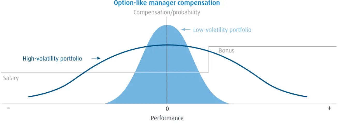
Figure 5 | Option-like compensation causes active managers to avoid low-volatility stocksSource: Baker and Haugen (2012) High-volatility portfolio
Salary
Performance
Bonus
Low-volatility portfolio Option-like manager compensation
Compensation/probability
pathological loss aversion. When all these human traits are put into the blender of the markets, the results are: • Overpricing of popular and glamorous companies • Market movements that overshoot (reach
unrealistically high or low levels) • Misperception of risk
…and so on. Overpricing of popular companies creates the value effect. Rallies and crashes that overshoot create the conditions for tactical asset allocation. The idea that low-volatility stocks have higher returns than high-volatility stocks is a little harder to explain, unless we can show that the effect is just a value or size effect, since volatility is easy to measure and investors hate risk of all kinds. As a result, we have to look beyond behavioral finance for the causes of the low-volatility anomaly.
Reasons for the low-volatility anomaly
While many anomalies in the market can be explained by behavioral finance biases, the most important ones — those that are large in economic impact, pervade many or most securities, and last a long time — demand explanations that do not simply assume that people are foolish. While there is a long literature documenting investor’s irrational preferences for stocks with lottery like
properties (see for example, Barberis and Huang (2008)), we’d be a lot more confident about investing in low-volatility stocks if we can find additional explanations that go beyond investor psychology. We’d prefer to see the anomaly anchored in more powerful “institutional arrangements,” where people are motivated by incentives or other powerful forces to make decisions that are irrational on the surface, but that are more rational when the institutional context is considered. When financial economists find a significant anomaly that persists over long periods of time, they tend to look for institutional arrangements as a possible source of the anomaly. After all, if a large enough group of people has an incentive to behave in a way, which appears irrational to others but is rational to them because of the incentive, they will do so — and push prices around, predictably, in such a way that other investors can trade profitably against them. This is what appears to be happening with the low-volatility anomaly. Baker and Haugen (2012) and Baker, Bradley, and Wurgler (2011, BBW) set forth compelling hypotheses regarding the impact manager incentives have on the returns of low-volatility stocks. Baker and Haugen simply note that low-volatility stocks provide fewer opportunities for managers to earn performance-based bonuses, so managers don’t buy them, as shown in Figure 5.
The authors write,
We see a manager compensation schedule whereby the manager is paid a base salary and then a bonus when performance is sufficiently high. Superimposed on the figure are two probability distributions: one for a volatile portfolio and the other for a less volatile portfolio. Obviously, the expected value of compensation increases if he/she sends a client the more volatile portfolio.
But while the amount of money managed under an incentive-pay scheme is large, it is not overwhelming. Incentive compensation is popular with hedge funds and some institutional long-only active equity funds, but is relatively rare in the “1940 Act” mutual funds used by individual investors and in defined-contribution retirement plans.
Managers do not need to be working for an explicit performance fee, however, in order to have an incentive to avoid low-volatility stocks. BBW find essentially the same embedded option in fixed-percentage (“flat”) fee contracts. They show that benchmark-aware active management could be the source of the superior returns of low-volatility stocks. Specifically, BBW show that if institutional active equity managers are rewarded for beating their cap-weighted benchmarks but punished for “tracking error” (the standard deviation of the difference between the active and benchmark returns), their incentives to overweight “cheap” stocks and underweight “expensive” stocks are properly aligned only for stocks with a beta near 1. Because of the relationship between a stock’s return and its alpha and beta, it turns out that, in order to outperform a rising market, the minimum alpha required by a high beta stock is actually negative compared to the minimum alpha, always positive, required by a low beta stock. Thus, managers are incentivized to overweight high-beta stocks they consider unattractive (negative alpha) and similarly they are motivated to underweight low-beta stocks they think are attractive (positive alpha). Thus, active equity managers may have a built-in bias toward high-risk stocks. In practice they hold about
53% of their trillions of dollars in U.S. active equity in stocks with betas greater than 1. This may be enough of a bias to explain the low-volatility effect.
Challenges to the low-volatility concept
With any investment strategy that has worked in the past, we have to ask, “Why might it not work in the future?” If the factors that caused it to work in the past can be expected to persist, then the strategy is likely to succeed in future time periods; if not, then it’s likely to fail.
Restricted borrowing
Now that some $6 trillion in assets (worldwide) are managed by hedge funds, which can borrow, one might wonder whether an anomaly that appears to be partly due to restricted borrowing will continue to exist.8
due to restricted borrowing will continue to exist.8
due to restricted borrowing will continue to exist. We note that the global capital market comprises some $200 trillion in investable assets. While $6 trillion might be enough to eliminate the anomaly if it were all devoted to buying low-volatility stocks and shorting high-volatility stocks, only a few managers do this. And a substantial fraction of the $6 trillion is invested in fixed income, having no effect on equity markets.
Meanwhile, “real money” investors — individuals, pension plans, endowments, foundations, and sovereign wealth funds — cannot borrow, other than by investing in leveraged hedge funds, a strategy that most investors undertake only on a limited basis because they are concerned about risk. The no-borrowing constraint, while relaxed a little in recent years, is thus mostly in effect.
Active equity managers hold
about 53% of their trillions of
dollars in U.S. active equity stocks
with betas greater than 1. This may
be enough of a bias to explain the
low-volatility effect.
Is low-volatility a crowded trade?
If enough investors are aware of the low-volatility anomaly and invest in funds designed to exploit it, the anomaly will go away, just as with any other “crowded trade.” There are now quite a few low-volatility funds on the market.
However, the amount of money flowing from active strategies to passive approaches is a tidal wave. These passive approaches include traditional cap-weighted index funds, ETFs, and fundamental indices. In the face of this movement, the trend toward low-volatility is minor and has a limited effect on security prices. Additionally, the flows toward passive, cap-weighted strategies serve to reinforce the biases that are built into cap-weighted benchmarks.
Will investors continue to be irrational enough?
For low-volatility investing to work, at least some investors need to be pursuing something other than risk-adjusted return; that is, some investors need to be irrational.9
be irrational.9
be irrational.
If all investors were rational they would have already arbitraged away any low-volatility opportunity as well as all other anomalies. They haven’t. Empirically, the value, small, momentum and low-volatility anomalies are as large as they’ve ever been. We know that this finding is counterintuitive given that business schools and the CFA program have been pounding the table for market efficiency and indexing for 30 or 40 years, but it’s true. Two of the top ten years (out of 86) for the value anomaly have been since the year 2000, as have two of the top ten for size, one of the top ten for momentum, and five of the top ten (out of 42) for volatility.
That is not the only evidence that markets continue to be as irrational as ever. The best-known examples of individual-stock irrationality — the Palm/3Com and Royal Dutch anomalies — are drawn from the last 15 years of history.10
of history.10
of history. The prices of mortgage-backed securities in the period leading up to the crash of 2008 are an even more recent example. As long as human beings are ruled by greed, fear, and other emotions, and trade based on incomplete information, we do not think that analysts will ever be put out of work by markets that are so efficient that they afford no profit opportunities.
Market distortions caused by benchmarking
The BBW argument that the low-volatility anomaly is caused partly by long-only active equity managers minimizing tracking error, depends on a lot of money being managed in that way. Assets have been moving away from this model in several directions: toward indexing, on the one hand, and toward hedge funds on the other. If long-only active equity management were somehow to disappear, the low-volatility anomaly might also. But that will likely never happen. And history shows that loss of market share by long-only active management is consistent with a robust low-volatility anomaly.
Every portfolio can be decomposed into two portfolios, the benchmark and a portfolio of active positions. Half the sum of the absolute values of the active portfolio weights is known as “active share” and, for long-only unlevered portfolios, is bounded between 0 and 1. Since the 1960s when consultants first started measuring managers using information ratio, the average “active share” has been declining as the average tracking error has also declined. What this means is that the proportion of benchmark in the typical active portfolio has increased while the proportion of truly active bets has decreased over the last 50 years. This has been the most fruitful period for the low-volatility anomaly. Thus, if the average “active share” continues to decline, low-volatility investing will probably thrive.
Empirically, the value, small,
momentum and low-volatility
anomalies are as large as they’ve
ever been. Two of the top ten years
(out of 86) for the value anomaly
have been since the year 2000,
as have two of the top ten for size,
one of the top ten for momentum,
and five of the top ten (out of 42)
for volatility.
Are there hidden style or sector biases in
the low-volatility strategy?
Any “factor tilt” or other systematic investment strategy is subject to the charge that it really earns its returns through exposure to other factors that are not revealed by, or known to, the manager. If that is the case, an investor might prefer to invest directly in the factors (using futures contracts, ETFs, or other methods). Low-volatility has some exposure to value and some to the small-cap factor. This is because, in some cases, the same behavioral factors — “glamour” and “lottery” — that cause a stock to be overpriced (and thus in the growth and large-cap categories) tend to add to its volatility. However, as Figure 6 shows, the value exposure of low-volatility only shows up in the high dividend yield, and not in the other traditional value indicators (price-to-earnings, price-to-sales, and price-to-cash flow ratios). The growth indicators show that low-volatility has lower historical earnings growth rates than the market, but not a lower ROE.
Figure 7 shows that the sector weights of low-volatility differ materially from those of the market. This is a good, not a bad, characteristic of the strategy. We are using the
volatility screen to pick sectors, not just individual stocks. This is one of the principal sources of alpha from the strategy. Some low-volatility managers try to neutralize these sector bets and wind up neutralizing much of the low-volatility performance advantage.
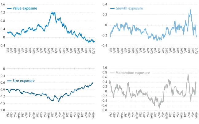
To delve further into the factor characteristics of the low-volatility style, we examined the exposures of a simulated low-volatility portfolio to several common factors; value, growth, size, and momentum. These exposures were calculated based on factors from Axioma’s Medium Horizon Fundamental risk model. The exposures displayed are the difference in weighted average exposure of the portfolio and the Russell 1000®
Indices. The results are shown in Figure 8 on page 9. The figure is presented in terms of standard deviation units. A value of zero indicates the portfolio has the same exposure as the benchmark, while a value of 1 would indicate an exposure a full standard deviation greater than the benchmark. For example, in the size graph, large size stocks have a positive coefficient and small stocks have a negative one. Therefore, a value of -1 means the low-volatility portfolio is significantly smaller than the benchmark.
Figure 6 | Fundamental characteristics of BMO low-volatility portfolio as of June 30, 2013
Holdings-based characteristics Large-cap low-volatility alpha Russell 1000® Index Weighted average market capitalization $38,992.9B $94,269.5B Median market capitalization $12,885.3B $6,476.4B
Number of securities 89 989
Dividend yield 2.37% 2.11%
Price-to-earnings FY1 estimate* 15.7x 14.7x
Price-to-cash flow* 9.5x 8.7x
Price-to-sales* 1.1x 1.4x
Historical 3-year sales growth 5.5% 11.0% Historical 3-year EPS growth 11.0% 16.7%
1-Year ROE 18.5% 17.5%
*Weighted harmonic average
Figure 7 | Sector weights of BMO low-volatility strategy as of June 30, 2013 Economic sector Large-cap low-volatility alpha Russell 1000® Index Difference Consumer discretionary 11.1% 13.0% -1.8% Consumer staples 22.9% 9.8% 13.2% Energy 0.7% 9.9% -9.2% Financials 23.6% 17.3% 6.4% Health care 20.5% 12.4% 8.1% Industrials 1.8% 10.9% -9.1% Information technology 4.0% 17.2% -13.1% Materials 0.4% 3.6% -3.2% Telecommunications services 3.7% 2.7% 1.0% Utilities 11.2% 3.4% 7.8%
1/8 2 4/8 3 7/ 84 10/ 85 1/8 7 4/8 8 7/ 89 10 /90 1/92 4/93 7/94 10/ 95 1/ 97 4/9 8 7/ 99 10 /0 0 1/0 2 4/0 3 7/ 04 10 /0 5 1/0 7 4/0 8 7/ 09 10 /10 Value exposure
Figure 8 | Factor exposures of low-volatility portfolio, 1982–2011 1.6 1.2 0.8 0.4 0 -0.4 1/8 2 4/8 3 7/ 84 10/ 85 1/8 7 4/8 8 7/ 89 10 /90 1/92 4/93 7/94 10/ 95 1/ 97 4/9 8 7/ 99 10 /0 0 1/0 2 4/0 3 7/ 04 10 /0 5 1/0 7 4/0 8 7/ 09 10 /10 Growth exposure 0.4 0.2 0 -0.2 -0.4 1/8 2 4/8 3 7/ 84 10/ 85 1/8 7 4/8 8 7/ 89 10 /90 1/92 4/93 7/94 10/95 1/97 4/9 8 7/ 99 10 /0 0 1/0 2 4/0 3 7/ 04 10 /0 5 1/0 7 4/0 8 7/ 09 10 /10 Size exposure 0 -0.3 -0.6 -0.9 -1.2 -1.5 -1.8 1/8 2 4/8 3 7/ 84 10/ 85 1/8 7 4/8 8 7/ 89 10 /90 1/92 4/93 7/94 10/95 1/97 4/9 8 7/ 99 10 /0 0 1/0 2 4/0 3 7/ 04 10 /0 5 1/0 7 4/0 8 7/ 09 10 /10 Momentum exposure 1.0 0.6 0.8 0.2 0.4 0 -0.2 -0.4 -0.8 -0.6
Source: BMO Global Asset Management Research Team, Axioma Inc. and Russell.
A negative exposure to momentum means that the low-volatility portfolio is exposed to a reversal effect (the opposite of momentum). Note that value and growth are not defined as mirror images of each other, so it’s possible for low-volatility to have both a negative value exposure and a negative growth exposure. This happened in 2011.
Interpretation of the factor loading graphs
We notice, in Figure 8, substantial change over time in the factor exposures of the low-volatility portfolio, and this fact calls out for explanation. By construction, the low-volatility portfolio will be where risk is not. For example, in 2000, at the peak of the tech bubble, investors were in love with risk. They caused risky (in this case, growth) stocks to have high prices and low expected returns, and low-risk (value) stocks to have low prices and high expected returns, value stocks dominated low-volatility portfolio holdings.
More recently, investors have shunned risk and this has caused risky assets to be cheap and have high expected returns. So low-volatility portfolios, which shun risk, are on the expensive side and have lower expected returns than they did on average historically. Low-volatility is, as a consequence, less “valuey” than it usually is — in fact, the loading on the value factor is
currently negative. Thus, the current time may not offer the highest premium of low-volatility over high-volatility that has ever been available, but it still offers a positive premium. That said, independent research has shown that this premium is resilient and has significantly benefited long-term investors.
By construction, the low-volatility
portfolio will be where risk is not.
Summary
Low-volatility investing is one of the largest and most surprising opportunities to earn excess returns (alpha) that has ever been identified. It is not just a statistical artifact. The size of the anomaly is economically very meaningful, with the lowest-volatility quintile of U.S. equities delivering a 5% per year alpha over 1970–2011. For comparison, Clifford, Kroner, and Siegel (2001) report that, over a considerably shorter period, 1980–2000, most of the very best active managers had much lower annual alphas. Out of the 495 funds they studied, only three had an alpha over 5% and only 43 had an alpha over 2%.11
only 43 had an alpha over 2%.11
only 43 had an alpha over 2%.
The continued existence of a low-volatility anomaly in the future is supported by the logic of benchmark-sensitive active equity management, which leaves low-volatility stocks undersubscribed and thus potentially priced for superior returns. Investors should seriously consider a substantial allocation to low-volatility equity funds.
1 Black’s collaborators Myron Scholes and Robert Merton won the
prize, but Black, who was acknowledged by the prize committee as an equal contributor to the Black-Scholes-Merton option pricing formula, did not live long enough to collect it. Nobel Prizes are not awarded posthumously.
2 See, for example, Shleifer and Vishny (1997).
3 See Ritter (2003). Other authors have made the same point. 4 Black’s words, describing Pratt (1967).
5 See Jahnke (1990, especially pp. 158-161) for a very thorough and
informative history of the frustrations that “quants” at his firm, Wells Fargo Investment Advisors (later Barclays Global Investors), had in getting funds launched that could exploit known market inefficiencies, including low-volatility. At Wells Fargo, the day the launch of their leveraged low-beta fund was canceled was known as “the day the alpha died.”
6 Including a well-regarded low-volatility paper, Haugen and
Heins (1975).
7 An excellent bibliography of behavioral finance is in Byrne and
Brooks (2009).
8 $2 trillion in investor capital, multiplied by a leverage ratio of 3:1. 9 Michael Brennan, a self-described “plain man” who often
finds neat answers to tough problems, argues the opposite. According to BBW: “In a simple equilibrium… along the lines of Brennan (1993), with no irrational investors at all, the presence of delegated investment management with a fixed benchmark will cause the CAPM relationship to fail. In particular, it will be too flat…” However, we’d note that an investor who hires delegated managers to pursue such a suboptimal strategy is irrational. See Brennan (1993).
10 3Com was a subsidiary of Palm Computing that was also traded
independently. In 2000, 3Com was priced so high, relative to Palm, that it was possible (by shorting 3Com) to buy a position in Palm ex-3Com (that is, the part of Palm that would remain if it sold 3Com in its entirety) at a negative price. This is one of the best-known “proofs” of irrational markets. Another is the fact that Dutch and British shares of Royal Dutch Shell, while providing claims to the same cash flows, have at times been more closely correlated to the Dutch and British market indices than they were to each other, providing an arbitrage opportunity.
11 Rankings calculated using spreadsheets provided by Clifford,
Kroner, and Siegel. References
Baker and Haugen (2012), “Low Risk Stocks Outperform within All Observable Markets of the World”, page 11. http://www.lowvolatilitystocks.com/wp-content/uploads/Low_ Risk_Stocks_Outperform.pdf.
Baker, Malcolm, Brendan Bradley, and Jeffery Wurgler. 2011. “Benchmarks as Limits to Arbitrage: Understanding the Low-Volatility Anomaly.” Financial Analysts Journal, Vol. 67, No. 1 Financial Analysts Journal, Vol. 67, No. 1 Financial Analysts Journal
(January/February).
Baker, Nardin L., and Robert A. Haugen. 2012. “Low Risk Stocks Outperform within All Observable Markets of the World.” Manuscript. http://papers.ssrn.com/sol3/papers.cfm?abstract_id=2055431. Barberis, Nicholas and Ming Huang, 2008, Stocks as Lotteries; The Implications of Probability Weighting for Security Prices, American Economic Review, 98:5, 2066-2100.
Economic Review, 98:5, 2066-2100. Economic Review
Black, Fischer. 1972. “Capital Market Equilibrium with Restricted Borrowing.” The Journal of Business, Vol. 45, No. 3. (July), pp.
444-455. http://www.mef.unina.it/download/finanza/Black_JB_72.pdf. Black, Fischer, Michael C. Jensen and Myron Scholes. 1972. “The Capital Asset Pricing Model: Some Empirical Tests,” in Studies in the Theory of Capital Markets, Michael C. Jensen, ed. New York:
Praeger, pp. 79–121.
Brennan, Michael. 1993. “Agency and Asset Pricing.” Working paper, University of California, Los Angeles (May), http://www.escholarship.org/uc/item/53k014sd.pdf.
Byrne, Alistair, and Mike Brooks. 2009. “Behavioral Finance: Theories and Evidence.” Research Foundation of CFA Institute, Charlottesville, VA, http://www.cfapubs.org/doi/pdf/10.2470/rflr.v3.n1.1.
Clifford, Scott W., Kenneth F. Kroner, and Laurence B. Siegel. 2001. “Analyzing the Greatest Return Stories Ever Told.” Investment Insights, Barclays Global Investors (now BlackRock), San Francisco,
Volume 4, number 1 (July).
Haugen, Robert A., and A. James Heins. 1975. “Risk and the Rate of Return on Financial Assets: Some Old Wine in New Bottles.” Journal of Financial and Quantitative Analysis, pp. 775–784.
Jahnke, William W. 1990. “The Development of Structured Portfolio Management: A Contextual View.” In Bruce, Brian R., editor,
Quantitative International Investing, Probus: Chicago, pp. 153-182.
Pratt, Shannon P. 1967 [2008]. “Relationship between Variability of Past Returns and Levels of Future Returns for Common Stocks.”
Business Valuation Review, Summer 2008, Vol. 27, No. 2, pp. 70-78. Business Valuation Review, Summer 2008, Vol. 27, No. 2, pp. 70-78. Business Valuation Review
Written in 1967 (unpublished).
Ritter, Jay R. 2003. “Behavioral Finance.” Pacific-Basin Finance Journal, Vol. 11, No. 4 (September), pp. 429-437. http://bear. Journal, Vol. 11, No. 4 (September), pp. 429-437. http://bear. Journal
warrington.ufl.edu/ritter/publ_papers/behavioral%20finance.pdf. Shleifer, Andrei, and Robert Vishny. 1997. “The Limits to Arbitrage.”
The Russell 1000® Index measures the performance of the large-cap segment of the U.S. equity universe. It is a subset of the Russell 3000® Index and
includes approximately 1,000 of the largest securities based on a combination of their market cap and current index membership. The Russell 1000®
represents approximately 92% of the Russell 3000® Index. The Russell 1000® Index is constructed to provide a comprehensive and unbiased barometer
for the large cap segment and is completely reconstituted annually to ensure new and growing equities are reflected. Investments cannot be made in an index.
All investments involve risk, including the possible loss of principal.
This is not intended to serve as a complete analysis of every material fact regarding any company, industry or security. The opinions expressed here reflect our judgment at this date and are subject to change. Information has been obtained from sources we consider to be reliable, but we cannot guarantee the accuracy. This publication is prepared for general information only. This material does not constitute investment advice and is not intended as an endorsement of any specific investment. It does not have regard to the specific investment objectives, financial situation and the particular needs of any specific person who may receive this report. Investors should seek advice regarding the appropriateness of investing in any securities or investment strategies discussed or recommended in this report and should understand that statements regarding future prospects may not be realized. Investment involves risk. Market conditions and trends will fluctuate. The value of an investment as well as income associated with investments may rise or fall. Accordingly, investors may receive back less than originally invested. Past performance is not necessarily a guide to future performance.
BMO Global Asset Management is the brand name for various affiliated entities of BMO Financial Group that provide investment management, retirement, and trust and custody services. Certain of the products and services offered under the brand name BMO Global Asset Management are designed specifically for various categories of investors in a number of different countries and regions and may not be available to all investors. Products and services are only offered to such investors in those countries and regions in accordance with applicable laws and regulations. BMO Financial Group is a service mark of Bank of Montreal (BMO).
For more information, visit us at bmogam.com.
Investment products are: NOT FDIC INSURED — NO BANK GUARANTEE — MAY LOSE VALUE.