econ
stor
Der Open-Access-Publikationsserver der ZBW – Leibniz-Informationszentrum Wirtschaft
The Open Access Publication Server of the ZBW – Leibniz Information Centre for Economics
Nutzungsbedingungen:
Die ZBW räumt Ihnen als Nutzerin/Nutzer das unentgeltliche, räumlich unbeschränkte und zeitlich auf die Dauer des Schutzrechts beschränkte einfache Recht ein, das ausgewählte Werk im Rahmen der unter
→ http://www.econstor.eu/dspace/Nutzungsbedingungen nachzulesenden vollständigen Nutzungsbedingungen zu vervielfältigen, mit denen die Nutzerin/der Nutzer sich durch die erste Nutzung einverstanden erklärt.
Terms of use:
The ZBW grants you, the user, the non-exclusive right to use the selected work free of charge, territorially unrestricted and within the time limit of the term of the property rights according to the terms specified at
→ http://www.econstor.eu/dspace/Nutzungsbedingungen By the first use of the selected work the user agrees and declares to comply with these terms of use.
zbw
Leibniz-Informationszentrum WirtschaftGönsch, Jochen; Steinhardt, Claudius
Article
Using Dynamic Programming Decomposition for
Revenue Management with Opaque Products
BuR - Business ResearchProvided in Cooperation with:
VHB - Verband der Hochschullehrer für Betriebswirtschaft, German Academic Association of Business Research
Suggested Citation: Gönsch, Jochen; Steinhardt, Claudius (2013) : Using Dynamic
Programming Decomposition for Revenue Management with Opaque Products, BuR - Business Research, ISSN 1866-8658, Vol. 6, Iss. 1, pp. 94-115, http://dx.doi.org/10.1007/BF03342744
This Version is available at: http://hdl.handle.net/10419/103721
1 Introduction
Over the past decade, the rapid development of e-commerce has opened up new possibilities, which have led to dramatic changes in how firms design, place, and price their products. In this paper, we focus on a sales strategy called opaque selling, which has become quite popular in service industries – especially in the travel industry. When selling an opaque product, the provider conceals some aspects of the offered service until the transaction has been completed. From a monopolistic point of view, opaque products can basically be seen as an addi-tional instrument of price discrimination that allows the supplier to provide a discount in order to attract additional low-value customers, but without exces-sively cannibalizing or diluting existing demand for fully specified products. As an alternative to this
market expansion, the provider could offer only a few discounts and raise the regular products’ prices in order to enhance the price discrimination of the existing customer base (e.g., Fay 2008).
The usage of opaque products has been shown to be successful in many practical applications. Specifical-ly in markets in which business travelers often make late purchases and the provider usually has to resort to some kind of temporal segmentation with ad-vanced purchase restrictions, opaque products can help effectively segment the market until the last minute before service provision without too much buy-down behavior. Segmentation is possible due to business travelers’ reluctance to risk accepting the “randomness” inherent in opaque products (e.g., Jiang 2007). Indeed, opaque products are often regarded as a more efficient alternative to
last-Using Dynamic Programming Decomposition
for Revenue Management with Opaque
Products
Jochen Gönsch, Department of Analytics & Optimization, University of Augsburg, Germany, E-mail: [email protected]
Claudius Steinhardt, Department of Analytics & Optimization, University of Augsburg, Germany, E-mail: [email protected]
Abstract
Opaque products enable service providers to hide specific characteristics of their service fulfillment from the customer until after purchase. Prominent examples include internet-based service providers selling airline tickets without defining details, such as departure time or operating airline, until the booking has been made. Owing to the resulting flexibility in resource utilization, the traditional revenue management process needs to be modified. In this paper, we extend dynamic programming decomposition techniques widely used for traditional revenue management to develop an intuitive capacity control approach that allows for the incorporation of opaque products. In a simulation study, we show that the developed ap-proach significantly outperforms other well-known capacity control apap-proaches adapted to the opaque product setting. Based on the approach, we also provide computational examples of how the share of opaque products as well as the degree of opacity can influence the results.
JEL-classification: C61, M11, M19
Keywords: revenue management, opaque products, capacity control, dynamic programming decomposi-tion
Manuscript received March 13, 2012, accepted by Karl Inderfurth (Operations and Information Systems) February 15, 2013.
minute selling (Jerath, Netessine, and Veerara-ghavan 2010). Examples of opaque products in practice include airlines that allow customers to book a flight from A to B on a specific date, but con-ceal schedule information, such as the exact depar-ture and arrival times, connections, transfers, and layover durations; hotel chains that conceal the specific hotel in which the customer will stay; and cruise lines that hide the cabin type or even the itin-erary until after purchase.
Opaque products’ popularity has been heavily driv-en by offers from intermediaries, such as Hotwire and Priceline, which multiple providers share. In addition to the concealed information described above, intermediaries usually hide the service pro-viders’ brand names (e.g., those of the airlines, rent-al firms, hotels, or cruise lines) when selling an opaque product. Many service providers currently tend to move customers of their traditional products back to company-managed direct distribution channels as well as to streamline prices and create price parity across these channels. Thus, the addi-tional usage of a completely separate, anonymous channel via intermediaries – which hide the provid-er’s identity by combining different providers’ prod-ucts into a single opaque product – allows providers to effectively post different prices simultaneously while maintaining price parity and control of full-information-posted price channels (e.g., Anderson 2009). Furthermore, a provider that does not pro-duce multiple, horizontally differentiated regular products even needs to utilize an intermediary in order to successfully introduce an opaque product (Fay and Xie 2008).
There has been increasing interest in opaque prod-ucts in the academic literature in the last few years. Most of the research on opaque selling with posted prices has concentrated on analyzing the general economic benefits of offering opaque products in a static setting and discussed how prices should be set compared to those of traditional products, mostly on the basis of stylized economic models. In this paper, we tackle the topic from a revenue manage-ment perspective in a dynamic setting based on capacity control, which is a key component of mod-ern revenue management. Basically, capacity con-trol is concerned with the task of optimally selling a network of perishable resources with a fixed capaci-ty over time by dynamically making products de-fined on this network available or unavailable to customers (e.g., Talluri and van Ryzin 2004). As
soon as opaque products are introduced, traditional optimization models, which are used to perform automated capacity control, can no longer be ap-plied due to the supplier-driven substitution possi-bilities inherent in opaque products.
Therefore, the contribution of this paper is the de-velopment of a new approach to capacity control, enabling the service provider to simultaneously offer both, opaque products and traditional ones. We show that this approach outperforms other well-known capacity control approaches adapted to the opaque product setting. Our approach builds on the well-known dynamic programming decomposition procedure; this procedure is not only state-of-the-art from a theoretical point of view, but also widely used for standard capacity control in commercial revenue management systems. Therefore, the re-sults are relevant to both research and practice. Moreover, service providers who already apply ad-vanced revenue management techniques and are considering introducing opaque products can im-plement this approach very easily. Based on the new approach, we are able to investigate some specific effects that arise in a dynamic setting when opaque products are introduced. In particular, we give ex-amples of how the degree of opacity can influence the revenue performance, and that the share of opaque products obtained from total sales is a criti-cal aspect with respect to overall revenue perfor-mance.
The paper is structured as follows: In section 2, we begin with a brief discussion of the existing litera-ture on and related to our topic. We then present the basic network dynamic programming formula-tion for the capacity control problem, including opaque products (section 3). In section 4, we analyt-ically show how to use dynamic programming de-composition in order to decompose the given capac-ity control problem. Moreover, we prove that im-portant results known from standard capacity con-trol also hold in the opaque setting. In section 5, the control mechanism resulting from the decomposi-tion is extensively investigated in a computadecomposi-tional study. We consider typical airline revenue manage-ment scenarios in order to show its practical ap-plicability and its relative performance compared to other potential control approaches. In addition, we analyze some specific effects arising from the intro-duction of opaque products. In section 6, we con-clude with a summary of the paper’s main results.
2 Related
literature
In the scientific literature, opaque products are usu-ally discussed from a perspective that could best be described as situated at the interface of economics, marketing, and operations management. Most of the work is concerned with the task of finding opti-mal selling strategies, especially optiopti-mal prices, in scenarios that allow for opaque selling. In most cases, static settings with an unlimited capacity are considered and stylized economic models are devel-oped.
Jiang (2007) investigated a monopolist’s different strategies by comparing the settings solely with regular products, solely with opaque products, and both product types simultaneously. He showed that opaque selling can be pareto-improving for both, customers and provider if customers’ valuations are quite differentiated. Furthermore, Fay and Xie (2008) incorporated capacity constraints and de-mand uncertainty. Fay (2008) investigated how product opacity affects the market in a competitive environment and analyzed a common intermedi-ary’s impact. Whereas he assumed there are two service providers and one intermediary, Shapiro and Shi (2008) extended his setting to an arbitrary number of competing providers; the total number of providers can be regarded as a proxy for the opacity level of the opaque product that the common inter-mediary offers. The authors showed that although the opaque product’s introduction increases compe-tition for the low-price segment, compecompe-tition for the market’s more lucrative segment – which the pro-viders serve directly by means of regular products – decreases. Jerath, Netessine, and Veeraraghavan (2009, 2010) investigated a related setting but con-sidered two subsequent periods. They specifically addressed the question of whether opaque products should be offered via the intermediary or whether the direct last-minute selling of regular products should be used in the last period. Post (2010) as well as Post and Spann (2011) investigated variable opaque products, which allow the customer to con-figure the amount of opaqueness to a certain extent. However, there are only a few papers from the tradi-tional revenue management stream of research that consider the impact that the introduction of opaque products has on established capacity control mech-anisms. Talluri (2001) investigated an airline com-pany whose customers are indifferent to the various itineraries serving the same market, as long as they are similar with regard to arrival/departure times
and price. The author suggested a deterministic model formulation of the problem and derived a bid price policy, assigning customers to specific itinerar-ies immediately after booking. Chen, Günther, and Johnson (2003) investigated various approaches to capacity control in air cargo revenue management, where flexibility also emerges from different routing options.
The literature on revenue management with flexible products is also related to our work: Flexible ucts can be seen as a generalization of opaque prod-ucts in the sense that the provider does not have to determine a flexible product’s full specification im-mediately after the sale, but can postpone this deci-sion even further, if necessary until shortly before service provision. Gallego and Phillips (2004) and Gallego, Iyengar, Phillips, and Dubey (2004) first introduced and investigated the concept of flexible products. Petrick, Steinhardt, Gönsch, and Klein (2012) further analyzed flexible products’ potential to compensate for imprecise demand forecasts. Petrick, Gönsch, Steinhardt, and Klein (2010) de-veloped several dynamic control mechanisms that allow for flexible products’ practical integration into existing capacity control systems. The idea of reve-nue management with flexible products has been adapted to several fields of application (e.g., Bartodziej and Derigs 2004; Bartodziej, Derigs, and Zils 2007; Spengler, Rehkopf, and Volling 2007; Müller-Bungart 2007; Kimms and Müller-Bungart 2007).
Regarding the optimization technique used in this paper, the literature on dynamic programming de-composition approaches for revenue management is of particular interest. Talluri and van Ryzin (2004) described the standard decomposition approach for the traditional revenue management setting, which is used to split the full network dynamic program into a number of single-leg problems that are usual-ly much easier to solve. This technique serves as a basis for the approach incorporating opaque selling, which is developed in this paper. A number of re-cent publications, for example, Liu and van Ryzin (2008), Miranda Bront, Méndez-Díaz, and Vulcano (2009), Zhang and Adelman (2009), Erdelyi and Topaloglu (2010), Kunnumkal and Topaloglu (2010), and Meissner and Strauss (2012) adapted dynamic programming decomposition to other settings, such as the choice-based network revenue management setting or overbooking settings.
revenue management, see the textbooks by Talluri and van Ryzin (2004) and Phillips (2005), as well as the surveys by Weatherford and Bodily (1992), McGill and van Ryzin (1999), as well as Chiang, Chen, and Xu (2007).
3
General notation and dynamic
programming formulation
We rely on the standard revenue management set-ting as introduced, for example, by Talluri and van Ryzin (2004), which can be stated as follows: There are l resources indexed by
\
1,!,l^
with ch denoting the total remaining capacity for eachh . The corresponding vector is denoted by
1, , l
c c
c ! . Furthermore, there are n products defined on that are indexed by "
\
1,!,n^
. The revenue obtained when selling one unit of product j" is denoted by rj. Requests for the products arrive throughout a common booking horizon, with all units of capacity remaining after its end being worthless. The booking horizon can be sufficiently discretized into T periods, so that there is at most one incoming customer request for each period t1,...,T. The probability of an arrival of a request for a product indexed by j in period t is denoted by p tjand 0
1 j
j p t p t
" is the probability of there being no incoming request. The periods are numbered backwards in time. Thus,1 t jt j D p U U
is the expected aggregated de-mand-to-come at the point in time t for a product indexed by j.The difference resulting from the introduction of opaque products compared to the standard case lies in the definition of the resource consumption. There are now potentially several specification options
j
% ! the provider can choose from after selling an opaque product indexed by j" . ! ` is the index set of all products’ specification options, where the consumption of an option with index
i! on a resource with index h is expressed by the parameter ahi. The corresponding vector is denoted by ai a1i,!,ali
. Note that any regular product indexed by j' can be modeled as a special case of an opaque product with %j' 1. Subse-quently, for the sake of simplicity, we refer to a re-source indexed by h as “resource h”. The same abbreviation is used for the other index sets.Now, let V
c,t be the maximum expected reve-nue-to-go from period t onward, assuming that
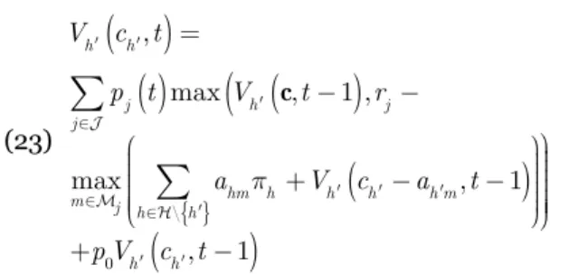
resource capacity c is left over. Then, the dynamic programming formulation of the capacity control problem with opaque products can be stated as the following Bellman equation (DP-op):
(1)
0 , max , 1 , max , 1 , 1 j j j j m m V t p t V t r V t p t V t ¬ ®
c c c a c " %The boundary conditions are V
c, 0 0 for cp0 and V
c, 0 d otherwise, because any remain-ing capacity at service provision is worthless and negative values of the remaining capacity are not allowed. The extension to the standard dynamic programming formulation (e.g., Talluri and van Ryzin 2004) is that we replace the revenue-to-go resulting from the acceptance of request j with the maximization term max , 1
j m
m%V c a t , because a decision has to be made regarding how to resolve opacity. That is, one of the specification options included in the set %j is selected in a revenue-maximizing way. The corresponding decision rule directly follows from the model by rearranging terms. An incoming request for an opaque product j is accepted if and only if
(2) min
\
, 1, 1
^
j j m m r V t V t p c c a % ,which means that there must be at least one specifi-cation option for which the opportunity cost does not exceed the revenue. In the case of acceptance, a potential specification m* with minimal oppor-tunity cost V c,t 1
V c a m*,t1 is selected and capacity is reduced accordingly. The traditional model and its related decision rule are obviously special cases of (1) and (2), because, if %j 1, the maximization and the minimization can be omitted in (1) and (2), respectively.
Note that formulation (1) is more closely related to the standard formulation without opaque products than to the dynamic programming formulation proposed by Gallego, Iyengar, Phillips, and Dubey (2004) for flexible products. In particular, from a technical perspective, (1) is not a special case of these authors’ model. This is because, with flexible products, the state space is modeled completely different. It does not include current remaining
capacities of the resources, but only stores the commitments that have been made by selling prod-ucts. Regarding these commitments, capacity is allocated only in the last stage of the dynamic pro-gram by solving a linear feasibility problem. This inhibits the direct application of resource-based decomposition approaches, which is possible in our model for opaque products, as we demonstrate in the next section.
4 Dynamic
programming
decomposition
Similar to the dynamic program in the traditional setting, DP-op – as given by (1) – is not solvable for most realistic resource networks due to the curse of dimensionality. Therefore, in this section, we show that the well-established idea of dynamic program-ming decomposition used in traditional network revenue management (e.g., Talluri and van Ryzin 2004: Chap. 3) can be transferred to the setting with opaque products. The main idea of dynamic pro-gramming decomposition can be summarized as follows: the network dynamic programming model is decomposed into a collection of single-resource dynamic programs, each of which is only one-dimensional and, therefore, avoids the curse of di-mensionality. Using these easy-to-solve dynamic programs, dynamic opportunity costs, which vary as a function of time and capacity, can be obtained and used for a price-based control policy. To account for the network structure, the decomposition uses static information from the optimal solution of an easier-to-solve network model, which is usually the well-known Deterministic Linear Program (DLP) assum-ing deterministic demand (e.g., Talluri and van Ryzin 2004: Chap. 3).
4.1 Derivation
Following the generic idea of dynamic programming decomposition (e.g., Liu and van Ryzin 2008), we approximate DP-op at a given resource ha by: (3)
\ ^ \ , h h, h h h h V t V c ta a Qc a x
c, h h
V c ta a is a dynamic, time- and capacity-dependent approximation of the value of capacity of resource ha and \ ^ \ h h h h c Q a
is a static linear ap-proximation of the other resources’ capacity. In our setting, we propose to obtain the values of Qh from
a generalization of the DLP that, to the best of our knowledge, was first presented by Talluri (2001) in the context of passenger routing (see section 2). In this model, as opposed to the standard DLP, the decision variables xjm have two indices, as they denote the number of expected future requests for opaque products that should be assigned to each of the specification options m%j. The optimization problem can then be formulated as follows ( DLP-op): (4)
, max j DLP j jm j m V t r x
c " % subject to (5) j hm jm h j m a x c b
" % for all h (6) j jm jt m x D b
% for all j" (7) xjm p0 for all j", m%j Compared to the traditional DLP model, in the ob-jective function (4), in the capacity constraints (5), and in the demand constraints (6) it is now neces-sary to additionally sum up over all specification options for each product. Again, the traditional setting is obviously a special case. Similar to the traditional decomposition approach, each Qh is taken from the optimal solution of DLP-op and corresponds to the dual variable, that is, the bid price associated with the capacity constraint for each resource h.Substituting the approximation (3) into the Bellman equation (1), we obtain (8)
\ ^
\ ^ \ ^
\ ^ \ \ \ 0 \ , max , 1 , max , 1 , 1 j h h h h h h j h h j h h m j h h h m h h h h hm h h h h h h h h V c t c p t V c t c r V c a t c a p t V c t c Q Q Q Q a a a a a a a a a a a a a ¬ ¬ ¸ ®® ¬ ®
" %with the boundary conditions V cha
ha, 0 0 for 0
h
c a p and V c
ha, 0 d otherwise. After some minor rearrangements, we have the following dy-namic program, which is one-dimensional with respect to capacity: (9)
\ ^
\ 0 , max , 1 , max , 1 , 1 j h h j h h j j h hm h h h m m h h h h V c t p t V c t r a V c a t p t V c t Q a a a a a a a a a a ¬ ¬ ®®
" %with the same boundary conditions as before. It can be shown that two of the most prominent results known from standard capacity control im-mediately carry over to the extended setting. In particular, we have Proposition 1.
\ ^ \ , h h, h h h h V t V c ta a Qc a b
c for all c 0p ,t1,..., ,T ha as well as Proposition 2.\ ^
\ , DLP , h h h h h h V c ta a Qc V t a
b c for all c 0p ,t1,..., ,T haThe proofs for Propositions 1 and 2 are given in Appendix A1 and A2, respectively. Proposition 1 means that the dynamic programming decomposi-tion – applied at a single resource ha while the val-ues of the remaining resources are approximated by the duals of DLP-op – provides an upper bound on the network dynamic programming model. This result has been shown analytically for other specific revenue management models (e.g., Zhang and Adelman (2009) for the derivation in choice-based revenue management) and holds in settings with opaque products as well. From Propositions 1 and 2, it follows that the dynamic programming decompo-sition leads to a tighter upper bound than the one obtained when simply using DLP-op.
4.2 Discussion
The result of the derivation of the dynamic pro-gramming decomposition approach for opaque products shows two specific and intuitive aspects of how opacity has to be taken into consideration. First, similar to the standard approach, which only considers regular products, dual values from the solution of the corresponding deterministic model are used to capture network effects; they are incor-porated by subtracting the value of capacity used elsewhere in the network from each product’s reve-nue. What is new in the setting with opaque prod-ucts is that the dual values from the DLP-op solu-tion are also used to obtain specificasolu-tion-dependent adjusted revenues, which is intuitive because the specification, which is chosen by the provider after sale, determines the capacity used elsewhere in the network.
Second, interestingly, it turns out that the decision problem on how to resolve opacity remains included in each of the resulting one-dimensional dynamic programs. Even though only a single resource ha is considered explicitly, all specification options are taken into consideration, whether they require ca-pacity on ha or not. This is reflected by the inner term \ ^
\ max , 1 j j h hm h h h m m r h ha Qa V ca a a a t ¬
® % in(9). More specifically, there can even be specifica-tion opspecifica-tions for opaque products that do not require the current resource at all. Consequently, their se-lection in the single-resource dynamic program will not lead to any changes in remaining capacity cha. Instead, the required resources’ static bid prices Qh capture the capacity consumption implied by the selection of such an option. Thus, in contrast to the standard decomposition, the static bid prices from the deterministic network model are not only incor-porated in an “AND”-fashion, reflecting the usage of multiple resources by a product, but also in an “OR”-fashion, reflecting the different specification options a product can use. This is illustrated in de-tail by the example given in Appendix A3.
4.3 Control mechanism
In line with the mechanism for the standard case, a control mechanism can be constructed based on the dynamic programming decomposition outlined above. Bid prices Qh are derived by solving DLP-op up-front. The approximation is then repeated at each resource ha of the network, obtaining a set of
one-dimensional value functions V c t hha
ha, , a (see (9)). In the value function at resource ha, the products’ revenues are reduced by the bid prices Qh of resources h hv a used elsewhere in the network, depending on the specification option. The re-source-specific value functions are then aggregated to form a dynamic approximation of the network value function
, h
h, h V t V c ta a a x
c . This implies that the opportunity cost of accepting a request for the opaque product j and selecting a specification option m is approximated by , 1 , 1 h h h h hm h V c t V c a t
. In thiscon-text, the used resource-specific value functions (9) can be further simplified by only considering those products that need capacity from the resource ha in at least one specification option. This leads to the following reformulation: (10)
\ ^
: 0 \ : 0 , max , 1 , max , 1 1 , 1 j res h h res j h h j m j h ma res j m hm h h h h m h h res j h h j m j h ma V c t p t V c t r a V c a t p t V c t Q a a a a a a a a a a a a ¬ ¬ ®® ¬ ®
" % % " %Considering the definition of opportunity cost based on (9) and (10), respectively, it is easy to see that
, 1 , 1 , 1 res res h h h h hm h h V c t V c a t V c t , 1 , h h hm j V c a t j m " % holds. Then,throughout the booking horizon, the decision to accept requests is made in a similar way as outlined in section 3 for the original dynamic program by condition (2). The only modification is that oppor-tunity costs are obtained from the value functions
,
res h h
V c t instead of the original dynamic program, leading to (11) min , 1
, 1 j res res j m h h h h hm h r V c t V c a t p
% .In the case of acceptance, a potential specification
* j
m % with minimal opportunity cost
, 1 , 1 res res h h h h hm h V c t V c a t
is selectedand capacity is reduced accordingly.
5 Computational
results
In this section, we perform a simulation study to investigate revenue management settings that in-clude opaque products. Our study is based on two basic network structures that are introduced in sec-tion 5.1. Structures of this kind occur directly or as a substructure in common airline networks. The structure of the second network has been adapted from the literature. In section 5.2, we investigate the performance of the dynamic programming decom-position approach proposed in section 4. Having shown that the approach is a reasonable method of capacity control, we are able to investigate several specific aspects and effects that result from integrat-ing opaque products into a capacity control settintegrat-ing in detail in sections 5.3 and 5.4. In particular, in section 5.3, we analyze the effect of systematically varying the share of opaque products. In section 5.4, we describe how the inherent flexibility, that is, the degree of opacity drives the obtainable revenue performance.
5.1 Simulation experiment design
The numerical experiments we conduct are based on two example airline networks.
Network 1 consists of three parallel flights with capacities of 40, 30, and 35 seats each. There are four booking classes on each flight (Y, M, B, and Q) and one opaque product, producing 13 products in total. The fares are 500, 417.50, 335, and 250, de-pending on the booking class. Any of the three flights can be assigned to a customer of the opaque product, but he pays only 150. On each flight, 10%, 20%, 20%, and 30% of expected demand is for booking class Y, M, B, and Q, respectively; the re-maining 20% of customers request the opaque product.
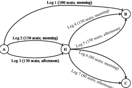
Network 2 is taken from the literature and was orig-inally proposed by Liu and van Ryzin (2008: §7.2). There are four cities A, B, C, and H, which are con-nected by seven flight legs with capacities of be-tween 80 and 150 seats (see Figure 1). We consider two booking classes Y and Q, producing a total of 27 regular and opaque products. The long-haul leg A-B can be booked for 900 and 540 in class Y and Q, respectively. The other single-leg flights are consid-ered short-haul and cost 500 in Y and 300 in Q. Four connecting itineraries are available from A via the hub H, priced at 800 and 480 in the two book-
Figure 1: Network 2
ing classes. In addition, five opaque products are offered in this network. There are three short-haul opaque products at a cost of 220 from A to H, H to B, and H to C, guaranteeing transportation on one of two possible itineraries, either in the morning or afternoon. Furthermore, there are two long-haul opaque products offering transportation from A to B and A to C that can be bought for 352. With respect to opacity in these products’ definition, besides the two connecting itineraries, customers flying from A to B can also be assigned to the direct flight. In case that, in total, expected demand equals the capacity on all flights, expected demand is calculated as fol-lows: demand for each connecting itinerary equals 30% of its total capacity and demand for the direct flights is set equal to the remaining capacity. On each itinerary, 30% of demand is for class Y, 40% for class Q, and 30% for an opaque product with the demand distributed evenly if there are multiple opaque products. Demand information is addition-ally given in tabular form in Appendix A4.
In our study, we assume the booking process to be time-homogeneous and the arrival rate is calculated accordingly from the expected demand value. Fur-thermore, in line with our model assumptions from section 3, the booking process is discretized into T periods, so that there is at most one incoming cus-tomer request in each period (e.g., Subramanian, Stidham Jr., and Lautenbacher 1999: section 3.2.1 for the discretization procedure). The resulting number of periods is 250 and 1500 in Network 1 and Network 2, respectively. We fix the number of
simulation runs, each of them representing a stream of product requests, for all considered scenarios to 100, and, depending on the matter of interest, re-port resulting aggregated performance indicators along with the corresponding confidence levels. If different control methods are compared, we use the same set of 100 streams of product requests for all of them. Furthermore, in both networks, we gener-ate additional scenarios by varying the demand intensity in advance in order to simulate different load factors. Therefore, we scale the expected de-mand using a parameter B
\
0.9,1.0,...,1.5^
, where B1 corresponds to the case that expected demand equals capacity on all flights, as described above.5.2 Performance evaluation of the dynamic programming decom-position
The purpose of this subsection is to indicate wheth-er the practical application of the proposed dynamic programming decomposition is reasonable in terms of relative performance compared to other typical model-based capacity control methods when gener-alized to the opaque product setting, as well as in terms of computational runtime.
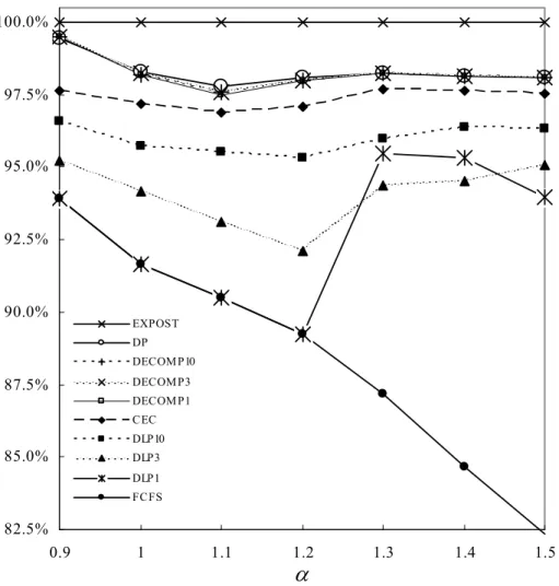
For Network 1, Figure 2 shows the revenue perfor-mance of all control methods tested relative to the perfect hindsight optimal revenue obtained with full information on demand (EXPOST). DP is the con-trol mechanism given by condition (2) based on the network dynamic programming model (1). The
Figure 2: Performance of the control methods relative to EXPOST (Network 1)
DECOMP#-variants implement the dynamic pro-gramming decomposition approach developed in section 4. The next four methods are immediate applications of DLP-op given by (4)-(7). CEC bases the acceptance of a request on the comparison of two optimal solutions of the model – one accepting the request and one rejecting it (see Bertsimas and Popescu (2003) for CEC in the standard setting). DLP# uses the dual variables from DLP-op as bid prices to implement standard bid price controls (e.g., Talluri and van Ryzin 2004: Chap. 3.3.1). A request is accepted if and only if its revenue is not less than the sum of the relevant bid prices in at least one specification option. FCFS is a simple first-come-first-served control, which accepts requests as long as they can be served with the remaining ca-pacity. In DECOMP# and DLP#, the number #
indicates how often the linear program is solved throughout the booking horizon. Within the control methods DECOMP1 and DLP1, the deterministic linear program is solved only once at the beginning. The dual variables associated with the capacity con-straints are then used to estimate the marginal value of capacity throughout the entire booking horizon. In methods DECOMP3 and DLP3, we partition the booking horizon into three evenly split periods and resolve the problem at the beginning of each period, using the remaining time, capacity, and estimated demand-to-come as input parameters. In DE-COMP10 and DLP10, 10 equal-sized periods are used.
First of all, Figure 2 clearly shows that the DECOMP approaches consistently produce almost the same revenues as DP. The number of reoptimizations has
82.5% 85.0% 87.5% 90.0% 92.5% 95.0% 97.5% 100.0% 0.9 1 1.1 1.2 1.3 1.4 1.5 EXPOST DP DECOM P10 DECOM P3 DECOM P1 C EC DLP10 DLP3 DLP1 FC FS
D
Figure 3: Performance of the control methods relative to EXPOST (Network 2)
no visible effect and the lines representing DP, DE-COMP1, DECOMP3, and DECOMP10 are so close that it is hard to distinguish between them. This is quite an impressive result since DP’s control deci-sions are perfect in the sense that they maximize expected revenue, given the available demand fore-cast. DECOMP1 is only significantly below DP at the 99% level of confidence for B1.1; however, the difference is only 0.5 percentage points. Further-more, it turns out that DECOMP1 performs signifi-cantly better than CEC, regardless of the demand intensity considered. Compared to the methods mentioned above, DLP10 trails about 1% behind. DLP3 is much less stable and about 2%-5% behind. DLP1 shows very high fluctuations: If the load factor is low (Bb1.2), it yields exactly the same low reve-nue as FCFS in all demand streams. This is because, although the total demand may exceed capacity, there is a positive contingent in the DLP model’s
optimal solution, even for low-value products. This leads to bid prices that allow for the acceptance of all requests, although the contingent in the solution may be very small. However, when the demand is stronger, DLP’s revenue sharply increases as it be-gins to reject some requests. Analyzing the benefit of the reoptimizations in detail confirms our observa-tion from Figure 2 that the effect of reoptimizing is negligible for DECOMP, as the confidence intervals comparing DECOMP1, DECOMP3, and DE-COMP10 are almost centered around 0. The corre-sponding results for B1.4 and confidence levels are given in Appendix A5.
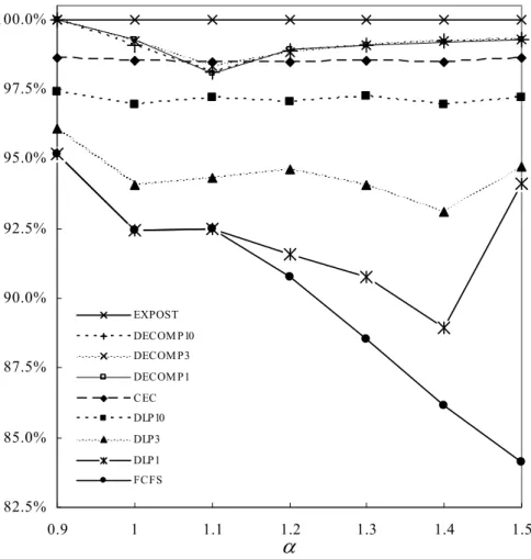
Likewise, Figure 3 shows the performance of the control methods for Network 2 relative to EXPOST. Note that the values for DP cannot be reported here, because the high dimensionality and size of the state space make its application impossible. The DE-COMP approaches usually produce the highest
rev-82.5% 85.0% 87.5% 90.0% 92.5% 95.0% 97.5% 100.0% 0.9 1 1.1 1.2 1.3 1.4 1.5 EXPOST DECOM P10 DECOM P3 DECOM P1 CEC DLP10 DLP3 DLP1 FCFS
D
enues, yielding over 99% of EXPOST’s revenue, and significantly outperform CEC. The impact of reop-timizing for the DLP approaches is much bigger for Network 2 than for Network 1. Regarding DECOMP, there is no significant advantage. However, our results (see also Appendix A5) indicate that reopti-mizations can – at least to a very small extent – help further improve the revenue. These figures suggest that, especially for DLP10, the revenue could be increased even more by further raising the number of reoptimizations. Nevertheless, it is important to note that regardless of the number of reoptimiza-tions, DLP will never outperform CEC in expecta-tion, because CEC can be regarded as resolving the linear program for every single customer and direct-ly deciding on the requests without being con-strained to additive bid prices. As DECOMP signifi-cantly dominates CEC, no reoptimization strategy will ever enable DLP to get close to DECOMP. The only exception is for B1.1. Here, the initial dual values of the DLP model that are used to calculate the adjusted revenues used in DECOMP1 are quite bad. In this case, the adjusted revenues are valid for only very few units of capacity, which leads to a revenue of 0.4% below that of CEC. However, when the adjusted revenues are updated during the book-ing horizon by resolvbook-ing the linear program, reve-nue increases and the gap between DECOMP and CEC can be reduced to 0.17%.
Overall, our results regarding the relative perfor-mance of the approaches are, by and large, in line with what is known from traditional revenue man-agement without opaque products. Even without reoptimizations, our decomposition approach con-sidering opaque products performs quite well. Its revenues are comparable to those obtained by DP
and it considerably outperforms the other methods, including CEC.
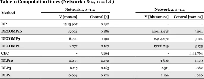
Table 1 shows computational time statistics for both networks for B1.4. With respect to DP-based methods, that is, DP, DECOMP1, DECOMP3, and DECOMP10, the column “V” shows the average time required for calculating the value function for all states. With regard to the latter three, this also includes the time to calculate the displacement-adjusted revenues; that is, the time required to solve the dual of the corresponding DLP-op. In case of CEC, nothing is computed in advance, as DLP-op needs to be resolved twice for every incoming re-quest. For DLP1, DLP3, and DLP10, the column “V” gives total computation times needed to solve DLP-op. For each method, the column “Control” refers to the time necessary to handle all the customer re-quests from one demand stream.
Table 1 shows that, although DP is still applicable in Network 1, calculating the value function is very time consuming. All other methods are tionally feasible for both networks. The computa-tional behavior of the decomposition approaches is identical to what is known from the standard setting without opaque products. The values from the col-umn “V” show that the DECOMP-variants are of course more time consuming than the DLP-op-based methods. However, as the resulting dynamic programs’ state space is one-dimensional with re-spect to capacity, computation time scales up linear-ly with the network size. Furthermore, as our inves-tigation from before suggests, it often seems unnec-essary to resolve the DECOMP approaches over time with respect to revenue performance. In this case, the value function of the DECOMP approaches could be completely pre-calculated. The times re-
Table 1: Computation times (Network 1 & 2, B1.4)
Method Network 1, B=1.4 Network 2, B=1.4 V [mm:ss] Control [s] V [hh:mm:ss] Control [mm:ss] DP 15:15.907 0.312 - - DECOMP10 15.024 0.186 1:00:11.438 3.201 DECOMP3 6.720 0.190 24:14.272 3.124 DECOMP1 2.277 0.187 17:08.249 3.135 CEC - 3.104 - 4:44.764 DLP10 0.233 0.172 3.806 1.120 DLP3 0.115 0.165 2.511 1.082 DLP1 0.064 0.170 2.199 1.090
quired to handle a request are rather similar and negligible for all methods, except, of course, CEC. Overall, from our investigation in this subsection, we can conclude that, for our example, the proposed decomposition approach performs particularly well in terms of realized revenue while, at the same time, our experiments demonstrate practical feasibility with respect to runtime. Therefore, with the decom-position, we seem to have found a reasonable meth-od to consider opaque prmeth-oducts in a revenue man-agement capacity control process. On this basis, we are now able to investigate several specific effects of opaque products in the following subsections. It is of course important to note that the results cannot be generalized with certainty and clearly depend on the setting. However, the results from this section regarding the relative performance of the various approaches are obviously in line with the results known to be valid for their counterparts in the standard setting. Therefore, we think that our re-sults are at least somewhat representative.
5.3 Share of opaque products
In this subsection, we analyze the effects of different shares of opaque products. As a point of departure, we use the products, prices, and demand shares from Network 1 with a demand intensity of B1.1. We use this intermediate demand intensity because, with it, capacity is scarce and, at the same time, it is optimal to accept quite a few opaque products. We now first remove the opaque products in order to construct a base case without any opacity. We then mimic the demand-side effects decision makers would potentially experience when deciding to in-troduce opaque products. First, the introduction of opaque products can lead to additional low-value demand from customers who had not purchased any of the offered products before (demand induc-tion). Second, customers who originally intended to buy a regular product could change their purchase behaviour and decide to buy the cheaper flexible product (cannibalization). In practice, the impact of demand induction and cannibalization is industry-specific and strongly depends on aspects, such as the products’ (relative) prices and the attractiveness of the opaque products.
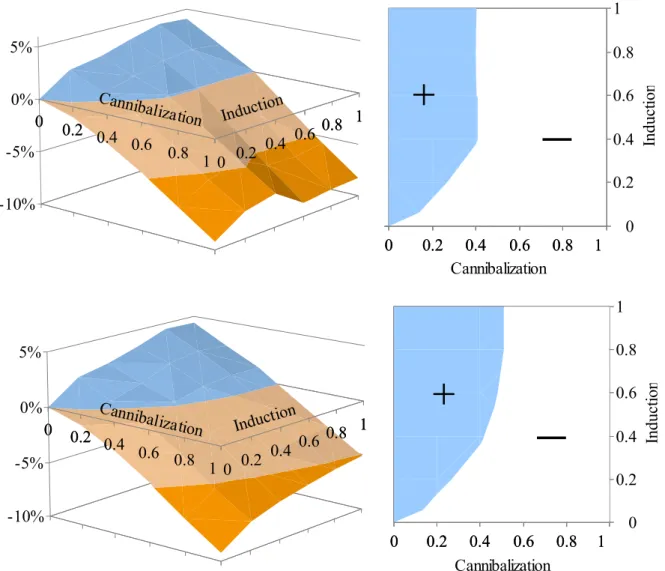
Figure 4 shows the revenues obtained with DP and DECOMP1 relative to the base case. In the graphs to the left, on one of the axes, we vary the level of de-mand induction and denote it relative to the num-ber of opaque product requests in the original
set-ting from section 5.1. More precisely, a value of zero refers to the base case without any opaque product requests, while a value of 0.5, for example, results in only half of the original opaque product demand. On the other axis, we vary the degree of cannibaliza-tion independently of induccannibaliza-tion. In this example, we assume that cannibalization always refers to only the cheapest regular product defined on the net-work, that is, class Q. A factor of zero means that there are no class Q-customers changing their de-mand behavior, while a value of 1 means that all original class Q-customers switch to the opaque product. The resulting cannibalized demand for the opaque product is added to the demand generated by demand induction. Note that, with a cannibaliza-tion of 0 and a demand induccannibaliza-tion of 1, we have the original setting that was investigated in section 5.2. The graphs on the right side in Figure 4 show the horizontal cross-section of the corresponding graph on the left, indicating the ranges of the values of cannibalization and induction for which the intro-duction of opaque products leads to a revenue im-provement (+) and those for which they lead to a loss (–).
We can observe from the results of DP in Figure 4 that a higher degree of demand induction leads to a better revenue performance, which is intuitive. However, the relationship is concave, as with a high number of induced opaque requests, capacity be-comes scarcer. On the other hand, a high cannibali-zation has a negative effect, as the opaque product is priced at 150 instead of 250 for the regular product. As DP would not be solvable for larger instances, it is important to get an idea of whether the decompo-sition, which we have identified as the best applica-ble approach in the previous subsection, leads to comparable results. The results for DECOMP1 in Figure 4 show that the dependency on induction and cannibalization is similar to DP in general. For example, the obtainable gain with a maximum in-duction rate or for a low inin-duction and a high can-nibalization rate are in a comparable range. Moreo-ver, the monotonicity properties are similar, except for the case of high cannibalization, where DE-COMP1 is not monotone in induction. This results from a disadvantageous set of bid prices from DLP-op used within DECOMP1, an effect that has already been discussed in section 5.2 and that can be miti-gated by applying reoptimizations. Overall, the re-sults from this example show that for a wide range of induction and cannibalization rates leading
Figure 4: Revenue depending on demand induction and cannibalization (upper row: DECOMP1, lower row: DP, Network 1)
to a specific share of opaque products, the introduc-tion of opaque products is advantageous in terms of revenue achieved. The range is similar but slightly smaller for DECOMP1 than for DP. However, these values are of course specific to our example and cannot be generalized.
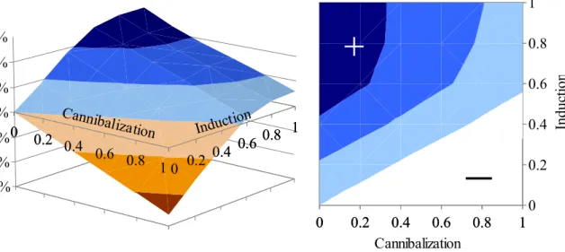
In Figure 5, we perform a similar analysis for Net-work 2, in which DP is, however, no longer tracta-ble. The results for DECOMP now show strict mon-otonicity in the parameters, as the influence of indi-vidual bid prices from DLP-op seems to be smaller. The possible overall gain of opaque products is big-ger than in Network 1. In particular, it is now always positive for high induction levels. As the relative
price difference compared to the cheapest regular product is smaller and the network is more com-plex, flexibility is obviously more valuable in this setting.
5.4 Degree of opacity
In this subsection, we investigate the degree of opacity’s influence on the revenues obtained. There-fore, we compare settings that differ only in the degree of flexibility inherent in their opaque prod-ucts. To construct the scenarios for this experiment, similar to section 5.3, we use the products, prices, and demand shares from Network 1 with a demand
0
0.2 0.4
0.6
0.8
1
0
0.2
0.4
0.6
0.8
1
-10%
-5%
0%
5%
0
0.2 0.4
0.6
0.8
1
0
0.2
0.4
0.6
0.8
1
Cannibali
zation Indu
ction
0
0.2
0.4
0.6
0.8
1
0
0.2
0.4
0.6
0.8
1
0
0.2
0.4
0.6
0.8
1
Cannibalization
In
d
u
ct
io
n
0
0.2 0.4
0.6 0.8
1
0
0.2
0.4
0.6
0.8
1
-10%
-5%
0%
5%
0
0.2 0.4
0.6 0.8
1
0
0.2
0.4
0.6
0.8
1
Cannibali
zation Indu
ction
0
0.2
0.4
0.6
0.8
1
0
0.2
0.4
0.6
0.8
1
0
0.2
0.4
0.6
0.8
1
Cannibalization
In
d
u
ct
io
n
Figure 5: Revenue depending on demand induction and cannibalization (DECOMP1, Network 2)
intensity of B1.1. To consider different degrees of flexibility, we now vary the number of flights between one and six with an identical per-flight capacity of ten seats and a constant number of 100 periods, allowing us to also calculate DP for most of the scenarios. Demand is generated exactly as de-scribed for Network 1 for each experiment. For ex-ample, when considering two flights, 20% of de-mand is for the opaque product and can be assigned to either flight. The remaining demand is flight-specific in booking classes Y, M, B, and Q for the two flights. When considering only one flight, demand is still generated as described for Network 1. As overall capacity is half of that compared to two flights, overall demand is half of that, too. From this de-mand, 80% is still flight-specific in Y, M, B, and Q. A total of 20% is still for the opaque product, which no longer really be considered opaque, as it can only be assigned to the sole flight. Comparing average per-leg revenues, the settings now only differ in the number of legs to which the opaque requests can be assigned.
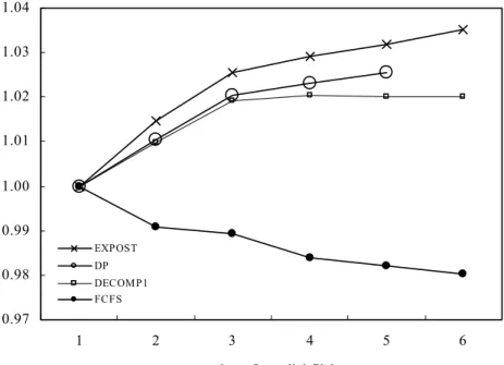
Figure 6 shows the revenues obtained with DP and DECOMP1 as well as the benchmarks FCFS and EXPOST relative to the revenues obtained with the respective method in the one-flight case. Thus, all methods “start” at 100% (1.00) for one flight. While FCFS’s revenue decreases to about 97% for six flights, we observe that the other methods’ revenues increase to 103.5% for EXPOST and 102% for
DE-COMP1 for six flights. DP attains about 102.5% for five flights, but is computationally intractable for more. For the latter three methods, increases in revenue are the strongest for one to three flights; DECOMP1 even levels off and stays more or less constant for more than three flights.
These observations can be explained as follows. FCFS is the only method whose revenues decrease with the number of flights, that is, when flexibility increases. This is due to FCFS’s general shortcoming of accepting too many low-value requests – in fact, accepting all it can. This shortcoming becomes even more severe with more flights, because the in-creased flexibility of opaque products means it can, and actually does, accept even more opaque re-quests. Thus, revenue decreases with increasing flexibility. This is a general property of FCFS; non-increasing revenues in the level of flexibility would show up in every setting where the opaque product is the cheapest one. In contrast, DP as the optimal control is – in expectation – never hurt by addition-al flexibility and revenues increase with the degree of flexibility as the opaque requests are used to miti-gate different levels of scarcity on the legs stemming from stochastic demand. Similarly, EXPOST’s reve-nues increase with the degree of flexibility as well. As this is the perfect hindsight control, this increase is not only in expectation, because no single in-stance can be constructed where EXPOST would make use of the flexibility although it should not.
0
0.2 0.4
0.6 0.8
1
0
0.2
0.4
0.6
0.8
1
-15%
-10%
-5%
0%
5%
10%
15%
0
0.2 0.4
0.6 0.8
1
0
0.2
0.4
0.6
0.8
1
Cannibali
zation
Indu
ction
0
0.2
0.4
0.6
0.8
1
0
0.2
0.4
0.6
0.8
1
0
0.2
0.4
0.6
0.8
1
Cannibalization
In
duc
ti
o
n
Figure 6: Revenue depending on number of parallel flights (one flight = 1.00)
The picture for DECOMP1 is more differentiated; two overlaying effects have to be distinguished here: On the one hand, an increased flexibility allows for better mitigating stochastic demand as explained above for EXPOST and DP. On the other hand, the more flights and, thus, the higher the degree of flex-ibility, the more alternative specification options have to be compared in the inner maximization of (9). Most of these specification options are only described approximately with the help of shadow prices from DLP-op. In our example, DECOMP1 is in fact identical to DP in the single-flight scenario. While the first effect increases revenue with flexibil-ity, the latter decreases the quality of the approxi-mation. Which effect prevails clearly depends on the scenario considered. Here, the first one seems to be stronger up to three flights; for more flights they cancel each other out. However, defining such a high degree of opacity would anyway cause a cus-tomer’s reaction in terms of demand induction and cannibalization as it was analyzed in section 5.3. Such effects have not been considered in this exam-ple as they are very much related to the specific industry setting. Nevertheless, it is likely that a very high degree of opacity would lead to a negative im-pact on revenue due to a much smaller demand induction.
Figure 7 shows the total computation time needed for processing one customer stream with DP and DECOMP1 in this experiment, depending on the number of flights. Note that the vertical axis has a logarithmic scale. In this graph, DP’s runtime is a straight line for two to five legs. This result clearly reflects the exponential growth of the DP’s number of states, and, thus, of the runtime as the number of flights increases. The slightly higher-than-expected runtime for one flight might be due to overheads, such as deciding on request acceptance. We consid-er measurement noise less likely, as the runtime closely matches that of DECOMP1 for one flight. Considering more flights, DECOMP1’s advantages are obvious: Although its runtime should theoreti-cally increase linearly in the number of flights as more of the single-leg dynamic programs have to be calculated, being less than a second, the runtime is so short that this effect is overshadowed by meas-urement noise. Therefore, no clear trend can be seen. Note that although DP’s runtime would not prevent application to six flights – as can be seen in the figure by extrapolating its line – its memory requirements also grow linearly with the exponen-tially growing number of states. Thus, the amount of physical RAM available prevents us from using DP with more than five flights.
0.97 0.98 0.99 1.00 1.01 1.02 1.03 1.04 1 2 3 4 5 6
number of parallel flights
EXPOST DP DECOM P1 FCFS
Figure 7: Computation time [hh:mm:ss] for 1-6 flights, logarithmic scale
6 Conclusions
In this paper, we consider revenue management with opaque products. Opaque selling is an addi-tional instrument of price discrimination that helps segment a market. However, the supplier-driven substitution inherent in these products must be reflected in the revenue management process as well. As the exact dynamic program describing ca-pacity control with opaque products is usually not applicable to problems of real-world size due to its multi-dimensional state space, we propose a quite intuitive approach for capacity control with opaque products. It is based on traditional dynamic pro-gramming decomposition heuristics widely used in theory and practice. We formally derive the ap-proach and analyze the resulting single-resource dynamic programs. It turns out that the decision problem of how to resolve opacity is still included in each program. However, the resulting cost of ca-pacity consumption for specification options that do not concern the current resource are completely approximated by the bid prices calculated by the corresponding linear program. We then show that our approximation implies a tighter upper bound on the optimal expected revenue than the well-known
DLP model adapted to the opaque product setting – an important result that is also known from the traditional setting without opacity.
In a numerical investigation, we further analyze the performance of our decomposition approach in the context of airline revenue management and com-pare it with traditional control mechanisms adapted to opaque selling. It shows that the decomposition approach’s revenue is comparable to that obtained by the full network dynamic program and signifi-cantly outperforms other approaches, such as DLP-based bid prices and certainty equivalent control. While DLP-based bid prices have to be frequently updated by resolving the linear program to adapt to demand and capacity utilization, solving the linear program underlying the decomposition only once up-front is sufficient. Reoptimizations slightly im-prove the revenue in only a few cases. With respect to memory and computation time, the decomposi-tion is comparable to the tradidecomposi-tional decomposidecomposi-tion approach without opacity and can thus be used for large networks.
Having identified the decomposition approach as the best applicable capacity control approach in opaque product settings so far, we use the approach
00:00:00,0 00:00:00,1 00:00:00,9 00:00:08,6 00:01:26,4 00:14:24,0 02:24:00,0 1 2 3 4 5 6
number of parallel flights
DP DECOMP1
to investigate some aspects that are particularly related to opaque products. In particular, we first investigate how the overall share of opaque products influences the results. When introducing opaque products, this share is mainly driven by demand induction as well as cannibalization effects. The results are meaningful in the sense that they basical-ly correspond to what can be expected. In general, we see a positive influence of induction and a nega-tive one of cannibalization with a few exceptions in our parallel flight settings arising from the heuristic nature of the control procedure. However, in the network setting, these heuristic effects do not show up. Overall, the experiment shows that the benefits of introducing opaque products in a capacity control setting strongly depend on the specific parameters of demand behavior. Second, we investigate how the degree of opacity drives the obtained results. In our examples, it turns out that the degree of opacity – modeled by the number of parallel resources that can be used to fulfill opaque requests – has a strong positive influence on revenue for moderate levels. However, for high levels of opacity, there are set-tings where the reverse effects arising from the heu-ristic nature of the decomposition compensate for the positive effect of an additional specification option.
We believe that the results presented in this paper are highly relevant for revenue management in practice. As opaque products are increasingly of-fered by companies that traditionally make use of revenue management, there is an urgent need to consider these innovative products in the capacity control methods used. This is important because only integrated methods, such as the decomposition approach presented, enable the supplier to fully benefit from the advantages of opaque selling. From our experiments, we conclude that in revenue man-agement settings, the introduction of opaque prod-ucts in an existing product portfolio followed by the application of the proposed decomposition ap-proach can be quite beneficial. However, it is im-portant to have an idea of what rates of demand induction and cannibalization can be expected as these were shown to be crucial for the success of opaque products. In this context, it is particularly important not to define a degree of opacity that is too high, as this may lead to a loss in revenue com-pared to a lower degree of opacity. This can be due to both the heuristic nature of the decomposition
approaches as well as to the quite likely and disad-vantageous reduction of the demand induction rate when the degree of opacity is too high.
Appendix
A1 Proof of Proposition 1
We make use of a decision vector u
\
0,1,...,!^
nfor each remaining capacity c, indicating whether a request arriving in the current period would be ac-cepted. The vector components indicate the provid-er’s acceptance decision as well as the specification to select after sale. That is, a request for product j is denied if uj 0 and accepted and specified as
!
j
u if uj p1. To be feasible with remaining capacity c, the vector must satisfy
(12)
\
^
^
u c u u a c £¦¦ ¤¦¦¥ ¬ b ® - ! % " 0,1,..., 0 j n j j j u u u j .With this set of feasible decision vectors -
c , the dynamic programming model can be reformulated as a linear program with decision variables
, 0 , V ct p ct (e.g., Adelman 2007): (13) minV
c,t subject to (14)
0 0 , , 1 1 , 1 j j j j j u j u j j u V t p t r V t p t V t v v p ¬ ® ¬ ®
c c a c " " for all t, ,c u-c . Likewise, the dynamic program that approximates the revenue at resource ha as given by (9) is formu-lated as a linear program, using decision variables
, 0 ,
h h h
V c ta a p c ta : (15) minV c tha
![Figure 7: Computation time [hh:mm:ss] for 1-6 flights, logarithmic scale](https://thumb-us.123doks.com/thumbv2/123dok_us/1428486.2691235/17.892.199.718.253.609/figure-computation-time-hh-mm-flights-logarithmic-scale.webp)