Network anomaly detection: a survey and comparative analysis of stochastic and deterministic methods

Boston University

OpenBU

http://open.bu.edu

BU Open Access Articles BU Open Access Articles

2013-12

Network Anomaly Detection: A

Survey and Comparative Analysis

of Stochastic and Determinis...

This work was made openly accessible by BU Faculty. Please

share

how this access benefits you.

Your story matters.

Version

Citation (published version): J Wang, D Rossell, CG Cassandras, I Ch Paschalidis. 2013. "Network

Anomaly Detection: A Survey and Comparative Analysis of Stochastic

and Deterministic Methods." Proceedings of the 52nd IEEE

Conference on Decision and Control, pp. 182 - 187.

https://hdl.handle.net/2144/18027

Network Anomaly Detection: A Survey and Comparative Analysis of

Stochastic and Deterministic Methods

Jing Wang,

Daniel Rossell,

Christos G. Cassandras,

and Ioannis Ch. Paschalidis

net-work anomaly detection. These methods cover most of the common techniques in the anomaly detection field, including Statistical Hypothesis Tests (SHT), Support Vector Machines (SVM) and clustering analysis. We evaluate all methods in a simulated network that consists of nominal data, three flow-level anomalies and one packet-flow-level attack. Through analyzing the results, we point out the advantages and disadvantages of each method and conclude that combining the results of the individual methods can yield improved anomaly detection results.

I. INTRODUCTION

A network anomaly is any potentially malicious traffic that has implications for the security of the network. It is of par-ticular importance to the prevention of zero-day attacks, i.e., attacks not previously seen, and malicious data exfiltration. These are key areas of concern for both government and corporate entities.

From the perspective of methodology, network anomaly detection methods can be classified as stochastic and de-terministic. Stochastic methods fit reference data to a prob-abilistic model and evaluate the fitness of the new traffic with respect to this model [7], [11], [12], [22], [29]. The evaluation can be done using Statistical Hypothesis Testing (SHT) [5], [13], [16], [19]. Deterministic methods, on the other hand, try to partition the feature space into “normal” and “abnormal” regions through a deterministic decision boundary. The boundary can be determined using methods like Support Vector Machine (SVM), particularly 1-class SVM [9], [21], [25], and clustering analysis [1], [6].

From the perspective of data, network anomaly methods can be either packet-based [7], [17], flow-based [2], [18] or window-based [12]. Packet-based methods evaluate the raw packets directly while both flow-based and window-based methods aggregate the packets first. Flow-based methods evalulate each flow individually, which is defined as a collec-tion of packets with similar properties. Flows are considered as a good tradeoff between cost of collection and level of detail [26]. Window-based methods group consecutive packets or flows based on a sliding window.

* Research partially supported by the ARO under grants W911NF-11-1-0227 and 61789-MA-MUR, by the NSF under grants EFRI-0735974, CNS-1239021 and IIS-1237022, by the AFOSR under grant FA9550-12-1-0113, and by the ONR under grants N00014-09-1-1051 and N00014-10-1-0952.

† Division of Systems Eng., Boston University, email:

[email protected].

‡Department of Electrical and Computer Eng., Boston University, email:

[email protected].

§Department of Electrical and Computer Eng., and Division of Systems Eng., Boston University, 8 Saint Mary’s St., Boston, MA 02215, e-mails:

[email protected]@bu.edu.

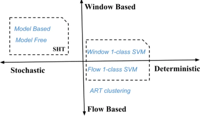
Flow Based ART clustering Flow 1-class SVM Window 1-class SVM Window Based Model Free Model Based Stochastic Deterministic SHT

Fig. 1. Relationships among the five evaluated methods.

The main goal of this paper is to discuss the advantages and distadvantages of each category of methods for different applications. This paper presents five methods, covering most of the categories discussed above, to the problem of host-based network anomaly detection and provides a comparative analysis. The first four methods are revisions of authors’ previous work with collaborators and the last method is new. The first two methods are based on SHT, utilizing results from Large Deviations Theory (LDT) [4] to compare cur-rent network traffic to probability laws governing nominal network traffic. The two methods fit traffic, which is a sequence of flows, with probabilistic models under i.i.d. and Markovian assumptions, respectively. We refer to these two

methods asmodel-free andmodel-based methods.

The next two methods are based on an 1-class SVM. In the first of the two methods, individual data transmissions from a given source are examined independently from neigh-boring transmissions, producing a flow-by-flow detector. In the other, sequences of flows within a time window are considered together to construct a window-based detector.

These two methods will be called flow 1-class SVM and

window 1-class SVM method, respectively.

Finally, we also present a clustering method based on Adaptive Resonance Theory (ART) [3], which is a machine learning technique originating in the biology field. This

algorithm, named ART clustering [23], partitions network

traffic into clusters based on the unique features of the network flows.

The relationships among these methods are depicted in

Figure 1. The flow 1-class SVM and the ART clustering

method are flow-based and capable of identifying individual network flows that are anomalous. By contrast, the remain-ing methods are window-based, under which the flows are grouped into a window based on their start time and only

suspicious windows of time can be identified as anomalous.

Model-freeandmodel-basedmethods are stochastic and the rest methods are deterministic.

A challenging problem in the evaluation of anomaly de-tection methods is the lack of test data with ground truth, due to the limited availability of such data. The most widely used labeled dataset, DAPRA intrusion detection dataset [14], was collected 14 years ago. Since then, the network condition has changed significantly. In order to address this problem, we developed software to generate labeled data, including a flow-level anomaly data generator (SADIT [28]) and a packet-level botnet attack data generator (IMALSE [27]). We evaluate all of our methodologies on a simulated network and compare their performance under three flow-level anomalies and one Distributed Denial of Service (DDoS) attack.

The rest of the paper is organized as follows. Section II describes the representation of network traffic data. Sec-tion III provides a mathematical descripSec-tion of the methods used to identify anomalies. Section IV provides an in-depth explanation of the simulated network and the anomalies. Section V presents the results of the five methods on the simulated network data. Finally, Section VI provides con-cluding remarks.

II. NETWORKTRAFFICREPRESENTATION

Let_S=_{s1_{, . . . ,s}|S|

}denote the collection of all packets

on the server which is monitored, where each element of_S

is one packet. We focus on host-based anomaly detection, in which case we only care about the user IP address, namely the destination IP addresses for the outgoing packets and the source IP addresses for the incoming packets. Denote

the user IP address in a packet si _{as x}i_{, whose format will}

be discussed later. The size of si _{is b}i

∈ [0,_∞) in bytes

and the start time of transmission isti

∈[0,_∞)in seconds.

Using this convention, the packet si can be represented as

(xi, bi, ti)for alli= 1, . . . ,_|S|.

Due to the vast number of packets, we consolidate this representation of network traffic by grouping series of

pack-ets into flows. We compile a sequence of packpack-ets s1 =

(x1, b1, t1), . . . ,sn = (xn, bn, tn) with t1 < _{· · ·} < tn

into a flow f = (x, b, dt, t) if x = x1 = · · · = xn and

ti

−ti−1 _{< δ}

F for i = 2, . . . , n and some prescribed

δF ∈(0,∞). Here, the sizebis simply the sum of the sizes

of the packets that comprise the flow. The valuedt=tn−t1

denotes the flow duration. The value t = t1 _{denotes the}

start time of the first packet of the flow. In this way, we

can translate the large collection of traffic packets _S into a

relatively small collection of flows_F=_{f1_{, . . . ,f}|F |

}. In some applications in which large numbers of users frequently access the server under surveillance, it may be infeasible to characterize network behavior for each user. Different methods deal with this dilemma differently.

For both statistical and SVM methods, we first dis-till the “user space” into something more manageable while enabling us to characterize network behavior of user groups instead of just individual users. For sim-plicity of notation, we only consider IPv4 addresses. If

xi = (xi1, xi2, xi3, xi4) ∈ {0,1, . . . ,255}4 and xj = (xj₁, xj₂, xj₃, xj₄)_{∈ {}0,1, . . . ,255_}4 _{are two IPv4 addresses,}

the distance between them is defined as: d(xi_,xj_{) =} P k=1,...,4256 4−k |xi k −x j

k|. This metric can be easily

ex-tended to IPv6 addresses if needed. Suppose _X is the set

of unique IP addresses in _F. We apply typical K-means

clustering on_X [8], [15]. For eachx_{∈ X}, we thus obtain

a cluster label k(x). Suppose the cluster center for cluster

kis x¯k_{, then the distance ofx to the corresponding cluster}

center isda(x) = d(x,x¯k(x)). Using user clusters, we can

produce our final representation of a flow as:

f = (k(x), da(x), b, dt, t). (1)

For the ART clustering method, distilling the user space

beforehand is not required. However, instead of using the IP

address directly, we use a compact representation. Letnf(x)

be the number of flows transmitted between the user with IP

addressxand the server. Definedb(x) =d(x,x∗),∀x∈ X,

wherex∗ _{is the IP address of the server we are monitoring;}

then the alternative flow representation we use is:

f = (nf(x), db(x), b, dt, t). (2)

III. ANOMALYDETECTIONMETHODS

A. Statistical Methods

Let h be the interval between the start points of

two consecutive time windows and ws be an

appro-priate window size; then the total number of windows

is nw = (t|F |−t1−ws)/h. We say flow fi = (k(xi_{), d} a(xi), bi, dit, ti)belongs to windowj if t1+ (j− 1)h_≤ti_{< t}1_{+ (j} −1)h+ws, ∀j= 1, . . . , nw. Letgi_{= (k(x}i_{), d}

a(xi), bi, dit)be the flow attributes infi

without the start timeti_and

Gj={g1,g2, . . . ,g|Gj|}be the

flows in windowj. Let_Gref be the set of all flows used as

reference. The window-based methods will compare_Gjwith

Gref for allj = 1, . . . nw. Both statistical methods we will

present in this section fall into this category and can work in supervised as well as unsupervised modes. In supervised

mode, _Gj is generated by removing suspicious flows from

a small fragment of data through human inspection. In unsupervised mode, we assume that the anomales are

short-lived thus_Gj can be chosen as a large set of nework traffic.

Since the approach introduced in what follows applies to all windows as well as to nominal flows, we use

G=_{g1_{, . . . ,g}|G|

} to refer to _Gref andGj,∀j= 1, . . . nw.

Suppose the range of da(xi),∀i = 1, . . . ,|G| is

[dmin

a , dmaxa ]. We can then define a discrete alphabetΣda=

dmin

a + (m+ 1/2)×(dmaxa −damin)/|Σda| m=0,...,|Σ_da|−1

for da(xi), where |Σda| is called quantization level. Σb

and Σdt can be defined similarly for b

i _{and d}i t. We

then quantize da(xi), bi and dit in gi to the closest

symbol in the discrete alphabet set Σda and Σb and Σdt,

respectively. Suppose the total number of user clusters

is K. Then we can denote the quantized flow sequence

G = _{g1_{, . . . ,g}|G|

} as Σ(_G) = _{σ(g1_{), . . . ,σ(g}|G|₎

},

discrete alphabet for quantization where each symbol in Σ corresponds to a flow state.

1) Model-free Method: In cases in which all flows em-anating from the server under surveillance are i.i.d., we

construct the empirical measure of flow sequence _G =

{g1_{, . . . ,g}|G|

}as the frequency distribution vector

EG(ρ) = 1 |G| |G| X i=1 1_{σ(gi) =ρ_}, (3)

where1_{·}denotes the indicator function andσ(gi_)denotes

the flow state in Σthat gi _{gets mapped to. We will denote}

the probability vector derived from the empirical measure of

the form in (3) asEG =

EG_(σ1_{), . . . ,}

EG_(σ|Σ|_{) .}

Let µ denote the probability vector calculated from the

reference flows_Gref. That is,µ(σ)is the reference marginal

probability of flow state σ. Using Sanov’s theorem [16],

[4], we construct a metric to compare empirical measures

of the form in (3) to µ, thus a metric of the “normality”

of a sequence of flows. For every probability vector ν

with supportΣ, letH(ν_|µ) =P

σ∈Σν(σ) log (ν(σ)/µ(σ))

be the relative entropy of ν with respect to µ. Allowing

η =_−n1log, where is a tolerable false alarm rate, then

themodel-free anomaly detector is:

I(_G) =1_{I1(EG)≥η}, (4)

whereI1(EG) =H(EG|µ). It was shown in [19] that (4) is

asymptotically Neyman-Pearson optimal.

2) Model-based Method: As an alternative to the i.i.d.

assumption on the sequence of flows under the model-free

method, we now turn to the case in which the sequence of flows adheres to a first-order Markov chain. The notion of

empirical measure on the sequence_G=_{g1, . . . ,g|G|_}must

now be adapted to consider subsequent pairs of flow states.

We assume no knowledge of an initial flow stateσ(g1)and

define the empirical measure on _G, under the Markovian

assumption, as the frequency distribution on the possible flow state transitions, EBG(σ i_,σj_{) =} 1 |G| |G| X l=2 1σ(gl−1) =σi,σ(gl) =σj , (5)

where1_{·}denotes the indicator function andσ(gl_)denotes

the flow state inΣwhichgl_{gets mapped to. We will denote}

probability matrices formed by the empirical measure in (5)

as EG_B=

EG B(σ

i_,σj₎

i,j=1,...,|Σ|.

In the following, we will refer to matrices of the form

Q = _{q(σi,σj)_}i,j=1,...,|Σ| as probability matrices with

support Σ_×Σ. By design, the empirical measures of the

form (5) are probability matrices with support Σ _× Σ.

Each probability matrix, under the Markovian assumption, is associated with a transition probability matrix of the form

{q(σj

|σi₎

}i,j=1,...,|Σ| where q(σj|σi) = q(σi,σj)/q(σi).

Here q(σi_{) =} P|Σ|

j=1q(σ

i_,σj_{)denotes the marginal}

proba-bility of flow state σi _inQ.

LetΠ=_{π(σi_,σj₎

}i,j=1,...,|Σ|denote, under the

Marko-vian assumption, the true probability matrix of sequences of

flows. As in the i.i.d. case, we compute Π via (5) from

Gref. Following a similar procedure as in the i.i.d. case, we

use an analog of the Sanov’s Theorem for the Markovian case, which appears in [4], as the basis for our model-based stochastic anomaly detector. For every shift invariant

probability matrixQwith supportΣ_×Σ, let

HB(Q|Π) = |Σ| X i,j=1 q(σi,σj) log q(σ j |σi₎ π(σj_|σi₎.

be the relative entropy ofQwith respect toΠ. Then in the

model-based method, the indicator of anomaly for_G is:

IB(G) =1{I2(EGB)≥η} (6)

whereI2(EG_B) =HB(EGB|Π)and η=

1

nlog withbe an

allowable false alarm rate. Again, the model-based detector

has been proved in [19] to be asymptotically Neyman-Pearson optimal.

B. 1-class SVM

We turn now to deterministic methods based on the construction of a decision boundary. We focus on one pop-ular technique named 1-class SVM [16], [24]. The premise behind 1-class SVM is to find a hyperplane that separates the

majority of the data_Z=_{z1_{, . . . ,z}|Z|

}from the outliers by

solving a Quadratic Programming (QP) Problem [19], [24]. The hyperplane can be generalized to a nonlinear boundary by mapping the inputs into high-dimensional spaces with a

kernel function K(_·,_·) [9]. There is a tunable parameter ν

effectively tuning the number of outliers.

1) Flow 1-class SVM: We consider a set of flows _G =

{g1_{, . . . ,g}|G|

} that need to be evaluated. According to (1),

each flow has the format ofg= (k(x), da(x), b, dt), which

has already provided a rather compact representation of network traffic. The only additional process required is to remove the label of the cluster each user belongs to. The

new data are: _Z = _{z1 _{= (d}

a(x1), b1, d1t), . . . ,z|Z| =

(da(x|Z|), b|Z|, d |Z|

t ). The reasoning for this is that, since

we are measuring departures from nominal users, the actual cluster a user belongs to is less important than the distance between the user the cluster center. Besides, as a categorical attribute, cluster labels make 1-class SVM method more unstable in practice. Besides, we choose the radial basis

function K(u,v) = exp ₋γ(u₋v)T(u₋v) as the

ker-nel function [16].

2) Window 1-class SVM: We combine the techniques described in Section III-A and the 1-class SVM into a

window-based 1-class SVM method. For each window j

with flows_Gj, we can get the model-freeempirical measure

EGj _{and the model-based empirical measure E}Gj

B. Let the

feature vector for window j be Yj ₌ n_EGj_,EGj

B,|Gj| o

. Let_Y =_{Y1_{, . . . , Y}|Y|

} be a time series consisting of the

features for all windows, then an 1-class SVM can be used

to evaluate_Y, resulting in a window-based anomaly detector.

Note that since the dimension of featureYj _{is usually very}

large, it often helps to apply Principal Component Analysis (PCA) [20] to reduce the dimensionality first.

C. ART Clustering

In this section, we present a clustering algorithm based on ART theory [3] and apply it to network anomaly detection. The algorithm first organizes inputs into clusters based on a customized distance metric. Then, a dynamic learning approach is used to update clusters or to create new clusters.

Assume a set of flows _F = _{f1, . . . ,f|F |_} with form

in (2). Similar to the statistical methods, we define gi =

(nf(x), db(x), bi, dit) to be the attributes in fi without the

start time ti _and

G is the counterpart of _F. Suppose gij

is the jth attribute of flow gi _{for all i = 1, . . . ,}

|G| and

j= 1,2,3,4. Defining fmin(j,G)andfmax(j,G)to be the

minimum and maximum of the set _{gij _:

∀i = 1, . . . ,_|G|},

we can normalize_G according to ˆgij = gij−fmin(j,G))

fmax(j,G)−fmin(j,G)

for all i = 1, . . . ,_|G|, and j = 1,2,3,4. In this section we

assume that the data in_G has already been normalized.

Define the distance metric

D(p,q) = m X j=1 _p j−qj 1₋vj 2 (7)

for two m-dimensional vectors p= (p1, . . . , pm) andq =

(q1, . . . , qm), wherev= (v1, . . . , vm)is a set of parameters

vj ∈ [0,1) that controls the vigilance in dimension j.

Let _Tk be the set of all flows in cluster k. Letting ck =

(nk_f, dk, bk, dk_t) represent the center of cluster k and cj_k be

itsj component. Let _C be the set of all cluster centers. For

everyc_{∈ C} and a prescribedr,

D(g,c)_≤r,g_∈Rm (8)

defines an ellipsoid inRm. A higher vigilance in one

dimen-sion means the ellipsoid is more shallow in this direction. The ART clustering algorithm is shown in Algorithm 1.

Initially _C is empty. For each flowgi_{∈ G}, we calculate the

set_Dwhich consists of all clusters whose ellipsoid defined

by (8) containsgi_{. SupposeE(g,c)is the Euclidean distance}

between g and c. If _D is not empty, gi _{is assigned to the}

cluster whose center has the smallest Euclidean distance

with gi _{and the corresponding cluster center is updated;}

otherwise a new cluster is created. Suppose that flowgi _will

be assigned to clusterk, letcj_k0 andcj_kbe thejth component

of the center of cluster k before and after the assignment,

then

cj_k0 = (p_×cj_k+gij)/(p+ 1),_∀j= 1, . . . , m, (9)

where p is the number of flows in cluster k before the

assignment. Because of the adaptive update (9), some as-signments may become unreasonable after update as some flows may become closer to other cluster centers. As a result,

the algorithm processes flows in_Gagain until an equilibrium

is reached.

Once a stable equilibrium is reached, small outlying clus-ters are identified as anomalous based on the rule

IA(Tk) =1{|Tk|< τ× |G|/|C|} (10)

where_IA(Tk) is an indicator of anomaly for Tk, τ ∈[0,1]

is a prescribed detection threshold,_|C| and_|G|are the total

Algorithm 1 ART clustering Algorithm

Require: Flow Data_G=_{g1_{, . . . ,g}|G|

} C=_Clast ={} while_{C 6}=_Clast do Clast=C fori= 1_{→ |G|}do D=_{c_{∈ C}:D(gi_{,c))< r} } if_|D|= 0 then C=_{C,gi_} else co= arg minc∈CE(gi,c) Tk ={Tk,gi},k is the index ofco inC.

Recalculate cluster center of_Tk using (9)

end if end for end while

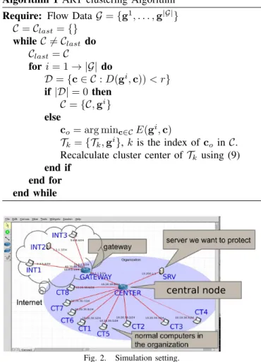
central node

Fig. 2. Simulation setting.

number of clusters and flows, respectively.τdetermines how

small a cluster must be to be considered as anomalous, thus it influences the number of alarms. We will discuss the

relationship ofτand the false alarm rate further in Section V.

IV. NETWORKSIMULATION

The lack of annotated data is a common problem in the network anomaly detection community. As a result, we developed two open source software packages to provide flow-level and packet-level validation datasets, respectively. SADIT [28] is a software package containing all the algo-rithms we described above. It also provides an annotated

flow record generator powered by the fs [26] simulator.

IMALSE [27] uses the NS3 simulator [10] for the network simulation and generates packet-level annotated data. Simu-lation at the packet-level takes more computation resources but can mimic certain attacks, like botnet-based attacks, in a more realistic way. We validate our algorithms with the help of these two software packages. The packets generated

by IMALSE, which is ofpcapformat [27], are transformed

into flow records first. Then the flows generated by SADIT and IMASLE are tested independently with each algorithm. The simulated network is partitioned into an internal network with a hub and spoke topology that connects to the Internet via a gateway (Fig. 2). The internal network consists

of 8 normal users (CT1-CT8) and 1 server (SRV) with some

A. Flow-level Anomalies

First, we generate a dataset with flow-level anomalies. The size and the transmission of the nominal flows for user

i is assumed to follow a Gaussian distribution N(mi, σi2)

and Poisson process with arrival rate λi, respectively. We

investigate three most common types of flow-level anomalies. The first one mimics the scenario according to which a network intruder or unauthorized user downloads restricted data. A previously unseen user who has a large IP distance to the rest of the users starts transmission for a short period. The

second one is a useriwith suspicious flow size distribution

characterized by a meanma_i higher than a typical valuemi.

Usually flows with substantially large flow size are associated with the situation when some users try to download large files from the server, which can happen when the attacker tries to download the sensitive information packed into a large file. The last one is a user increasing its flow transmission

rate to an unusual value λa

i, which could be indicative of

the user finding an important directory on the server and downloading, repeatedly, sensitive files within that directory.

B. Packet-level Anomalies

A second anomalous dataset is created using the tool IMALSE [27]. The nominal traffic is generated using the

on-off application in NS3 [10], [27] in which the user sends

packets fortonseconds and the interval between two

consec-utive transmission is tof f. The traffic is a Poisson process,

which means the on time and off times are exponentially

distributed with parameter λon andλof f, respectively.

We assume there is a botnet in the network. There is a botmaster controlling the bot network and a Command and Control (C&C) server issuing control commands to the bots. In our simulation, both the botmaster and C&C server

are the machine INT2in the Internet, and CT1-CT5 in the

internal network have been infected as bots. We investigate a DDoS Ping flood attack in which each bot sends a lot

of ping packets to the server SRV upon the request of the

C&C server, aiming to exhaust the bandwidth of SRV. The

attack is simulated at the packet-level and the data are then transformed into flow records using techniques described

in Section II. With appropriate δF, the ton becomes the

flow duration of nominal flows and the tof f determines the

flow transmission rate of nominal flows. The initiating stage of the attack is similar to the first case in the previous section. During the attack, both the flow transmission rate and the flow size of the bots may be affected. First, the flow

transmission rate is increased as the bots ping SRV more

frequently. Second, the ping packets have different sizes from normal network traffic. Also, consecutive ping packets may be combined together if they are sent over a short time interval. The resulting flows may be very large in size if these combinations are common or very small otherwise, depending on the attack pattern.

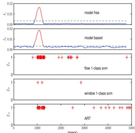
0.00 0.01 0.02 I1 model free 0.00 0.01 0.02 I2 model based 0 1 IS flow 1-class svm 0 1 IS window 1-class svm 0 1000 2000 3000 4000 5000 time(s) 0 1 IA _ART

Fig. 3. The results of five methods in the atypical user case.

V. RESULTS

A. Flow-level Anomalies

1) Atypical User: Figure 3 shows the response of all methods described above when there is an atypical user trying to access the server between 1000s and 1300s. For window-based methods, the interval between the starting

point of two consecutive time windows ish= 30s and the

window size is chosen as ws = 200s, so there is overlap

between two consecutive time windows. We also distill the

user space by usingK-Means clustering with 3 clusters. The

quantization levels for flow size, distance to cluster and flow

duration are 3, 2, 1, respectively, thus_|Σ_|= 18. Thex-axis

in all graphs corresponds to time (s) and the total simulation time is 5000s. The first two graphs depict the entropy metric

in (4) and (6) of the model-free andmodel-based methods,

respectively. For both graphs, the green dashed line is the

threshold when the false alarm rate is= 0.01. The interval

during which the entropy curve is above the threshold line (the red part) is the interval the method reports as abnormal.

The x coordinates of the red points with a ‘+’ marker

correspond to the start point of the flow or the window the

method reports as abnormal. The parameter ν for the flow

1-class SVM and window 1-class SVM is 0.002 and 0.1,

respectively. The thresholdτ for ART clusteringis0.05.

We can observe from Figure 3 that stochastic methods,

including ourmodel-freeandmodel-based methods, tend to

produce more stable results in the sense that they generate

fewer false alarms. At the same time, theflow 1-class SVM

andART clusteringmethods, both of which are flow-based, can provide higher identification resolution in the sense that they can identify the suspicious flows, which is beyond the

capabilities of the stochastic methods. In thewindow 1-class

SVM method, we can tune the window size to adjust the

tradeoff of resolution and stability. However, the window

size in the model-free andmodel-based methods has to be

reasonably large since the optimality of the decision rule (4) and (6) relies on the assumption of a large flow number in each window.

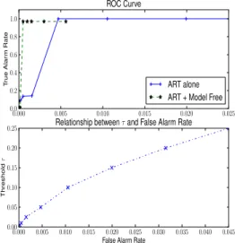
This observation indicates that these methods are com-plementary to each other. One way to combine them is

to use stochastic methods and window-based deterministic methods to get a rough interval of an anomaly. Then, only the flows that are both identified as suspicious by flow-based deterministic methods and belong to the interval need to be further evaluated. The first subfigure in Figure 4 shows the Receiver Operating Characteristic (ROC) curve of the

ART clusteringmethod, which is a flow-based method, and

the combination of the ART clustering and the model-free

method. The ROC curve has been substantially improved after combining the two methods. The second subfigure in

Figure 4 shows the relationship between the threshold τ

defined in (10) and the false alarm rate. The x-axis is the

false alarm rate and y-axis corresponds to the threshold. As

we can see, the false alarm rate increases when the threshold increases and they are almost linearly related to each other.

0.000 0.005 0.010 0.015 0.020 0.025 0.030 0.035 0.040 0.045

False Alarm Rate

0.00 0.05 0.10 0.15 0.20 0.25 Threshold τ

Relationship betweenτand False Alarm Rate

0.000 0.005 0.010 0.015 0.020 0.025 0.0 0.2 0.4 0.6 0.8 1.0 T rue Alar m Rate ROC Curve ART alone ART + Model Free

Fig. 4. ROC curve and relationship ofτand the false alarm rate for ART.

2) Large File Download: Figure 5 is the output of all methods in the case where a user doubles its mean flow size between 1000s and 1300s. Again, the first two graphs show

the entropy curve and threshold line of the model-free and

model-based methods. The total simulation time is 5000s.

The common window parametershandwsare the same as

in the previous case. The false alarm rate is = 0.01 for

bothmodel-freeandmodel-based methods. The parameterν

forflow 1-class SVMandwindow 1-class SVMis 0.0015 and

0.1, respectively.τ = 0.01for ART clustering.

3) Large Access Rate: Figure 6 shows the response of

model-free, model-based, window 1-class SVM and ART clustering methods when a user suspiciously increases its access rate to 6 times of its normal value during 1000s and 1300s. The total simulation time is 2000s. The parameters for the algorithms are the same in the atypical user case.

Note that flow 1-class SVM cannot work for this type

of anomaly since it is purely temporal-based. The flow itself does not change but its frequency does. There is no way to identify the frequency change by just observing the

individual flows with representation in (1). ART clustering

works fairly well for this case because the attacker will have

larger nf(x) as it transmits more flows. Interestingly, the

model-based and model-free methods can work very well

0.0 0.1 0.2 I1 model free 0.0 0.1 0.2 I2 model based 0 1 IS flow 1-class svm 0 1 IS window 1-class svm 0 1000 2000 3000 4000 5000 time(s) 0 1 IA ART

Fig. 5. The results of five methods in the large file download case.

since the portion of traffic originating from the attacker changes, influencing the empirical measure defined in (3) and (5). The two methods will not be effective in the very rare case when all users increase their rate by the same ratio synchronously. 0.00 0.01 0.02 I1 model free 0.00 0.01 0.02 I2 model based 0 1 IS window 1-class svm 0 500 1000 1500 2000 time(s) 0 1 IA ART

Fig. 6. The results of five methods in the large access rate case.

B. DDoS Attack

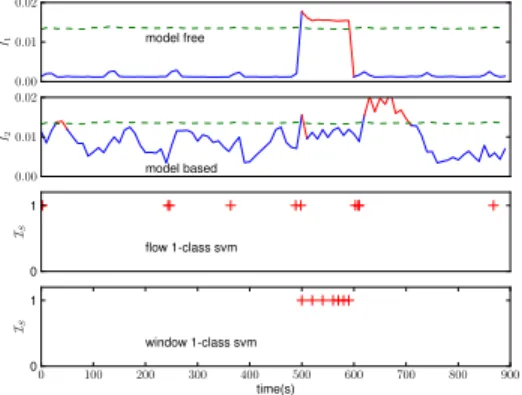
Figure 7 shows the response of model-free,model-based,

window 1-class SVM andflow 1-class SVM methods when

there is a DDoS attack targeting SRV between 500s and

600s. The total simulation time is 900s. For window-based methods, the interval between consecutive time windows is

h= 10sand the window size isws= 100s. The false alarm

rate for themodel-freeandmodel-based method is= 0.01

andν= 0.05 forwindow SVM.

Since the nominal traffic in IMALSE is generated based on

an i.i.d assumption, it is hard for the model-based method

to capture a Markov model. Yet, the model-based method

still detects the start and the end of the attack, during which

the transitional behavior changes the most. Model-free and

window 1-class SVM are more stable while theflow 1-class

SVM method provides higher resolution.

The ART clustering method is also not suited to detect these type of attacks because the unsupervised learning model is based on the assumption that malicious network traffic represents a small percentage of total network traffic. A DDoS attack generates a large number of packets and without some prior knowledge of good or bad network traffic,

theART clusteringalgorithm cannot distinguish between the nominal and abnormal flows. It is also the reason for the

relatively unsatisfactory performance of theflow 1-class SVM

method. However, window 1-class SVM is not affected by

this because despite the large number of abnormal flows, the number of abnormal windows is still very small.

0.00 0.01 0.02 I1 model free 0.00 0.01 0.02 I2 model based 0 1 IS flow 1-class svm 0 100 200 300 400 500 600 700 800 900 time(s) 0 1 IS window 1-class svm

Fig. 7. The results for DDoS attack.

VI. CONCLUSION

We presented five complementary approaches, based on SHT, SVM and clustering, that cover the common techniques for host-based network anomaly detection. We developed two open source software packages to provide flow-level and packet-level validation datasets, respectively. With the help of these software packages, we evaluated all methods on a simulated network mimicking typical networks in organizations. We consider three flow-level anomalies and one packet-level DDoS attack.

Through analyzing the results, we summarize the advan-tages and disadvanadvan-tages of each method. In general,

deter-ministic and flow-based methods, such asflow 1-class SVM

andART clustering, are more likely to have unstable results with higher false alarm rates but they can identify abnormal flows, namely they have better resolution. Stochastic and

window-based methods, such as our model-free and

model-based methods, could yield more stable results and detect temporal anomalies better, but they have relatively poor res-olution as they are not able to explicitly detect the anomalous network flows. In addition, deterministic and window-based

methods, likewindow 1-class SVMoffer parameters to adjust

the tradeoff of resolution and stability. This observation suggests that combining the results of all, instead of just using one method, can yield better overall performance.

REFERENCES

[1] M. R. Anderberg. Cluster analysis for applications. Technical report, DTIC Document, 1973.

[2] G. Androulidakis and S. Papavassiliou. Improving network anomaly detection via selective flow-based sampling. Communications, IET, 2(3):399–409, 2008.

[3] G. A. Carpenter and S. Grossberg. ART 2: self-organization of stable category recognition codes for analog input patterns. Applied Optics, 26(23):4919–4930, 1987.

[4] A. Dembo and O. Zeitouni.Large deviations techniques and applica-tions, volume 38. Springer, 2009.

[5] A. B. Frakt, W. C. Karl, and A. S. Willsky. A multiscale hypothesis testing approach to anomaly detection and localization from noisy tomographic data. IEEE transactions on image processing : a publication of the IEEE Signal Processing Society, 7(6):825–37, Jan. 1998.

[6] G. Gu, R. Perdisci, J. Zhang, W. Lee, et al. Botminer: clustering analysis of network traffic for protocol-and structure-independent botnet detection. InProceedings of the 17th conference on Security symposium, pages 139–154, 2008.

[7] I. Hareesh, S. Prasanna, M. Vijayalakshmi, and S. M. Shalinie. Anomaly detection system based on analysis of packet header and payload histograms. In Recent Trends in Information Technology (ICRTIT), 2011 International Conference on, pages 412–416. IEEE, 2011.

[8] J. A. Hartigan and M. A. Wong. Algorithm AS 136: A K-Means Clustering Algorithm.Journal of the Royal Statistical Society. Series C (Applied Statistics), 28(1):pp. 100–108, 1979.

[9] T. Hastie, R. Tibshirani, J. Friedman, et al. The elements of statistical learning: data mining, inference, and prediction, 2001.

[10] T. R. Henderson, M. Lacage, G. F. Riley, C. Dowell, and J. B. Kopena. Network simulations with the ns-3 simulator. SIGCOMM demonstration, 2008.

[11] A. Lakhina, M. Crovella, and C. Diot. Mining anomalies using traffic feature distributions. InACM SIGCOMM Computer Communication Review, volume 35, pages 217–228. ACM, 2005.

[12] W. Lee. Information-theoretic measures for anomaly detection. Pro-ceedings 2001 IEEE Symposium on Security and Privacy. S&P 2001, pages 130–143, 2001.

[13] E. L. Lehmann and J. P. Romano. Testing statistical hypotheses. Springer, 2005.

[14] R. Lippmann, J. Haines, D. Fried, J. Korba, and K. Das. The 1999 DARPA off-line intrusion detection evaluation. Computer networks, 34, 2000.

[15] S. P. Lloyd. Least squares quantization in pcm. IEEE Transactions on Information Theory, 28:129–137, 1982.

[16] R. Locke, J. Wang, and I. Paschalidis. Anomaly detection techniques for data exfiltration attempts. Technical Report 2012-JA-0001, Center for Information & Systems Engineering, Boston University, 8 Saint Mary’s Street, Brookline, MA, June 2012.

[17] M. V. Mahoney and P. K. Chan. PHAD : Packet Header Anomaly Detection for Identifying Hostile Network Traffic. (1998):1–17, 2001. [18] C. Manikopoulo. Flow-based Statistical Aggregation Schemes for Network Anomaly Detection. 2006 IEEE International Conference on Networking, Sensing and Control, pages 786–791, 2006. [19] I. Paschalidis and G. Smaragdakis. Spatio-temporal network anomaly

detection by assessing deviations of empirical measures.Networking, IEEE/ACM . . ., 2009.

[20] K. Pearson. Liii. on lines and planes of closest fit to systems of points in space.The London, Edinburgh, and Dublin Philosophical Magazine and Journal of Science, 2(11):559–572, 1901.

[21] R. Perdisci, G. Gu, and W. Lee. Using an Ensemble of One-Class SVM Classifiers to Harden Payload-based Anomaly Detection Systems.

Sixth International Conference on Data Mining (ICDM’06), pages 488–498, Dec. 2006.

[22] I. Perona, I. Albisua, and O. Arbelaitz. Histogram based payload processing for unsupervised anomaly detection systems in network intrusion.Proc. of the 14th . . ., 2010.

[23] D. Rossell. An ART Network Anomaly Detection Tool. http://

people.bu.edu/drossell/network.html, 2012.

[24] B. Schölkopf, J. C. Platt, J. C. Shawe-Taylor, A. J. Smola, and R. C. Williamson. Estimating the Support of a High-Dimensional Distribution, July 2001.

[25] T. Shon and J. Moon. A hybrid machine learning approach to network anomaly detection. Information Sciences, 177(18):3799–3821, 2007. [26] J. Sommers, R. Bowden, B. Eriksson, P. Barford, M. Roughan, and

N. Duffield. Efficient network-wide flow record generation, 2011. [27] J. Wang. IMALSE: Integrated MALware Simulator and

Emu-lator. http://people.bu.edu/wangjing/open-source/

imalse/html/index.html, 2012.

[28] J. Wang. SADIT: Systematic Anomaly Detection of Internet

Traf-fic. http://people.bu.edu/wangjing/open-source/

sadit/html/index.html, 2012.

[29] X. Zhang, Z. Zhu, and P. Fan. Intrusion detection based on the second-order stochastic model.Journal of Electronics (China), 24(5):679–685, Sept. 2007.