Agricultural Trade Liberalization and Poverty in Tunisia: Micro-simulation in a General Equilibrium Framework
33
0
0
Full text
(2) Abstract The study tries to answer the following questions: Will exposure to world agricultural prices generate more poverty or less? To what extent will households be affected by changes in agricultural trade polices? Do multilateral agricultural liberalization matter more than bilateral changes? Results of simulations using a computable general equilibrium (CGE) model linked to household survey data suggest that trade liberalization has only modest effects on the level of GDP, but it has a substantial effect in reducing poverty. Moreover, the combined effects of global and domestic liberalization are more pro-poor than the effect of domestic liberalization alone. As a net importer of agricultural commodities, Tunisia may be expected to experience terms-of-trade losses from higher world agricultural prices. However, given Tunisia’s significant agricultural import protection policies, it is expected that the agricultural sector will lose from trade liberalization that removes this protection. Keywords: Tunisia, agriculture, trade liberalization, general equilibrium model, microsimulation, poverty. JEL Classification: F1, I3, Q1, C68. 2 This work was carried out with financial and scientific support from the Poverty and Economic Policy (PEP) Research Network, which is financed by the Australian Agency for International Development (AusAID) and the Government of Canada through the International Development Research Centre (IDRC) and the Canadian International Development Agency (CIDA). The authors would like to acknowledge the work of Mrs. Sinda Ben Redjeb in the preparation of the data underlying the micromodule and poverty indicators. Many thanks are due to an anonymous referee for his valuables comments on earlier drafts.
(3) 1.. Introduction Determining the pattern and trends in poverty are central in policymaking and policy. reform in developing countries. Several policies that have undergone reforms, such as food price subsidies, general cash transfers, and expansion in public sector employment, have traditionally been justified as initiatives for supporting the needy. Trade policies and external shocks are also seen as a way of tackling poverty given their impact on stakeholders through various transmission channels: employment, prices, assets, and transfers. Accordingly, and in addition to their effects on sectoral demand for labor, particularly in those sectors that employ the poor, the manner by which trade liberalization affects prices will have an important bearing on income and expenditures and, directly or indirectly, on welfare measures. Thus, trade policies affect poverty through their effects on economic growth in one hand as well as through their distributional effects on the other. Tunisia is about to start implementing a new agreement on trade in agricultural products with the European Union (EU) under the association agreement signed in 1995, simultaneous to its participation in the World Trade Organization (WTO) as a member country involved in the multilateral negotiation on agricultural trade under the Doha Development Agenda (DDA). The aggregate impact of trade liberalization is likely to be positive, but like other major changes in economic policy, agricultural trade liberalization, may have some negative effects. Generally, trade liberalization presents both challenges and opportunities for developing countries in general and households (especially the poorest ones), in particular. More specifically, any new multilateral trade agreement on agricultural products under the Doha Round will lead to a reduction of protection and public support for agriculture in developed countries. Results from several models focusing on multilateral agricultural trade liberalization (e.g. Goldin and Knudsen, 1990; Goldin and Winters, 1992) provide evidence that poor households in developing countries may lose because of their status as net buyers of food and the induced upward effect on world food prices (Chaherli, 2002). Consequently, the effects of multilateral liberalization could eventually be much larger than those to be found under unilateral liberalization1. More generally, and according to Anderson (2003), agricultural trade liberalization alters relative product prices, which in turn affects factor prices. Hence its net effects on poverty reduction also depend on domestic product price changes and how they affect domestic factor prices, on the price and quantity of food available for consumption, and its eventual effect on real individual and household incomes. If the price changes are pro-poor, then they will tend to reinforce any positive growth effects 1. See for instance Hamilton and Whaley (1984) and Gibbon and Ponte (2005). 3.
(4) of trade reform on the poor. The outcome also depends on the extent to which changes occur in border measures and complementary domestic policies. The include the following: if the price changes create new markets that are pro-poor; if the price changes stimulate the poor to respond to altered prices; if the second-round spillover effects are pro-poor; if any transitional unemployment is minimized; if government revenues increase in such a way that it leads to pro-poor public expenditure; and if the vulnerability of the poor is reduced. Given that Tunisia’s agricultural sector currently enjoys substantial protection, additional broad-based trade liberalization will likely have a detrimental impact on some classes of households, including the bulk of the poor population. Two major questions rise: How will the Tunisian economy be affected by the new expected agreements on agricultural trade liberalization, both at the bilateral and multilateral levels? How will households react to these macro changes? Accounting for the effects of trade policy reform and external shocks on the distribution of welfare among individuals and households has long been on the agenda of economists. However, doing it satisfactorily has proved difficult, though progress in economic analysis and the increasing availability of micro-economic household data has helped to ease this difficulty. This study uses a static CGE model and micro-simulation techniques of Tunisia as a laboratory for analyzing alternative trade reforms. In order to focus on agriculture and issues of poverty, the model uses a relatively detailed treatment of agricultural production, trade instruments, and factor markets. The analysis begins by simulating a removal of all tariffs on industrial products imported from the EU as specified in the partnership agreement signed between the two parties. The second simulation looks at the combined effects of trade provisions specified in the first scenario with a phasing-out of tariffs on Tunisian imports of agricultural products originating from the EU. The third simulates the impact of a maximum unilateral trade liberalization scenario by offering the same tariff removal to imports from the rest of the world (ROW). The last scenario, adds to the previous one, where world prices increase as an expected result of any potential agreement on multilateral agricultural trade liberalization under the DDA. 2.. Background Tunisia has achieved a relatively impressive record of poverty reduction over the past. five decades, reducing the poverty incidence (using the national line poverty) from 40 percent in 1960 to 11 percent by 1985 and further to 7.4 percent by 1990. Poverty slightly increased. 4.
(5) in 1995 (8.1%2) but resumed its decline in 2000 where its incidence attained its lowest level (4.1%). In addition, income distribution improved until 1990 as the Gini coefficient dropped from 0.434 in 1985 to 0.401 in 1990, increased to 0.417 in 1995, and dropped again to 0.409 in 2000 (World Bank, 2003). Hence, the last decade had been characterized by two distinct patterns. The first half was marked by an increase in poverty, the result of a prolonged drought that led to a severe drop in agricultural production over 1993-95. This, in turn caused deterioration in the income of rural poor households more significantly than those of other households, who rely more on non-agricultural income. The second half of the decade was characterized by a reduction of poverty as a result of growth acceleration (5.6 % for GDP and 7.8% for agricultural output on average)3. Moreover, the reduction of poverty incidence over the past decades is also attributed to the coherent social policy implemented in the country since its independence. In fact, and even after the adoption of the structural adjustment program since the mid-80s, government expenditures on health and education sectors still accounted for 7.8 percent of GDP in 1995 (World Bank, 1995). Poverty is primarily a rural phenomenon in Tunisia. In 2000, the incidence of rural poverty was 8.3 percent compared to 0.8 percent in metropolitan areas and 2.3 percent in other urban areas. With less than 40 percent of the total population, rural areas accounted for 74 percent of the poor in 2000 compared to 76 percent in 1990 (World Bank, 2003). Poor rural households engaged in production activities typically have access to land, but their land holdings are small (averaging 2 hectares), rarely irrigated, and often exhibit low productivity, especially in rain-fed areas. The urban poor are mostly wage earners in low-skill occupations, or unemployed. Unemployment in Tunisia is estimated at 15 percent (National Institute for Statistics INS, 2000a). The results of the last survey of households’ expenditures showed an improvement in the average yearly expenditures by capita. According to the INS (2003), this figure reached 6.5 percent at current prices and 3.6 percent at constant prices over the period 1995-2000. Moreover, the increase has been more important in the rural areas (10%) than in the urban areas (5.9%), which led to a reduction in the gap of expenditure levels between the two areas. However, the annual expenditures per capita in rural areas represented only 58 percent of the level of yearly expenditure per capita in urban areas in 2000 (48% in 1995). In addition, the results of the 2000 household survey revealed that the lowest level of expenditures concerns households where the heads are unemployed, followed by those who are working in agricultural sector as wage-workers.. 2. Using the World Bank’s poverty line, the results are different from those estimated by NIS (World Bank, 2003). 3 World Bank (2003) 5.
(6) Despite the relatively high level of diversification of the Tunisian economy, the agricultural sector remains economically and socially important given its role in employment, regional equilibrium, and social cohesion (It contributes less than 15 percent to Tunisia’s GDP and accounts for around 20 percent of the total employment). The agricultural sector in Tunisia is characterized by a relative specialization in fruit, horticultural, and livestock production, which together contribute up to 80 percent of the total agricultural and fisheries value-added, but it is still vulnerable to limitations in natural resources and recurrent droughts. Food processing contributes nearly 10 percent to Tunisia total exports. Olive oil is by far the main exported agricultural product and represents 30 percent of food and agricultural exports. Fish and seafood products represent the second highest traded commodity with almost 20 percent of total food processing exports, while fruit exports, essentially dates and citrus, are third. On the other hand, agricultural and food imports, represent also around 10 percent of the total Tunisian imports of commodities. The structure of food processing imports reveals the chronic dependence on cereal imports as well as sugar and vegetable oils. With the implementation of the Agricultural Structural Adjustment Program (ASAP) since 1986, Tunisia began the liberalization of its agriculture sector with the objective of improving its competitiveness as well as its adjustment to the requirements of international markets. Thus, with the exception of wheat, agriculture activities have been substantially liberalized, subsidies on inputs have been practically eliminated, and the marketing boards have partially lost their monopolies. While the price of water for irrigation is still subsidized, it continues to be adjusted progressively. Production prices are freely determined, except for a few products where prices remain administrated (such as milk and cereals). However, the government still intervenes in the determination of market prices. Accordingly, when market prices for agricultural products4 increase above a given level, maximum price levels are fixed by the government either at the wholesale or retail level. This policy, inscribed within an objective of controlling inflation, has adversely affected farmers’ incomes during the last few years, and especially the small farmers. Despite the successive reductions in food subsidies, in the frame of the ASAP, food subsidies still represent 2 percent of government expenditures. The most subsidized products are cereals (absorbing more than 65% of total food subsidies), followed by vegetable oil (30%) and milk (5%). Given its importance in the Tunisian economy, agriculture currently benefits from substantial protection compared with the rest of the economy. Two instruments are still used for protection from external competition: tariff and non-tariff barriers. Overall, the nondiscriminatory rates (MFN) applied by Tunisia remain among the highest in the world. The 4. Mainly for vegetable and meat products 6.
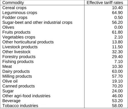
(7) economy-wide average level of protection reached 34.5 percent in 2002 against only 12.8 percent in the same year for other countries with intermediate income levels. Moreover, MFN rates have slightly evolved since the beginning of the 1990s, whereas they have been reduced by more than 40 percent on average in the other countries with intermediate income levels (Chemingui and Lahouel, 2004). For agricultural and food products, they are still highly protected even with the implementation of the partnership agreement with the EU in 1996 as the agreement has bearing only on non-agricultural manufacturing goods. Thus, imports of agricultural and food products is currently governed by the commitments undertaken by Tunisia within the multilateral framework of the GATT agreement in 1994. Accordingly, and while all quantitative restrictions are supposed to be converted to advalorem tariff rates, consolidated tariff rates have been fixed at very high levels. Currently, nominal protection is very high for agricultural and food products with an average of 89 percent and 72 percent respectively. However, these tariff rates vary highly across products. They are relatively high for fruit, forestry products, tobacco, meat, dairy products, cereals processing, canned products, and beverages. But they are lower for cereals, livestock, oils and sugar. For these four categories, together accounting for 60 percent of Tunisian imports of agricultural and food products, lower tariffs are applied under the preferential quota systems. Higher tariff rates are applied for imports exceeding the level of the quota. Table 1 shows 2001 data for tariff effectively applied on agricultural and food products. Table 1: Applied tariff rates for agriculture and food processing products in 2001 (in %) Commodity Effective tariff rates 10.40 Cereal crops 64.90 Leguminous crops 0.50 Fodder crops 56.20 Sugar-beet and other industrial crops 0.00 Olives 61.80 Fruits products 2.10 Vegetables crops 13.80 Other horticultural products 11.50 Livestock products 32.30 Other livestock 29.40 Forestry products 7.10 Fishing products 10.30 Meat 63.00 Dairy products 57.70 Milling products 19.10 Olive oil 70.20 Canned products 24.00 Sugar 46.00 Other agri-food industries 53.20 Beverage 58.00 Tobacco industries Source: Authors’ calculations using INS (2002). Even with the introduction of tariff-equivalent for non-tariff barriers (NTBs) under the GATT agreement, Tunisia is still using NTBs in the regulation of its agricultural and food 7.
(8) imports. Accordingly, public monopolies on the import of some agricultural and food products (e.g. the Tunisian Office of Commerce, the Oil Office et al.) represent the main tool of protection for most imported agricultural and food products in the country. The tariff equivalent of NTBs provides an indicator for the scale of this type of protection. Using the approach developed by Baldwin (1989), an estimation of the tariff equivalent of NTB for the main agricultural products imported by Tunisia was carried out by Chemingui and Dessus (1999) using data for the year 1992. Out of 19 agricultural and food products studied, six showed significant levels of tariff equivalents. Sugar had the highest non-tariff protection, with a tariff equivalent of 28 percent, followed by hard wheat (20%). The other protected products were barley, soft wheat, vegetable produce and canned goods. Currently, Tunisia is implementing both its association agreement with the EU and its GATT/WTO commitments in the Uruguay Round5. The EU is the major trading partner of Tunisia, accounting for 76 per cent of Tunisia’s two-way trade. This dependence is primarily due to industry – 80 percent of imported industrial products come from Europe and 78 percent of Tunisia’s industrial exports are for the European market – but much of the same holds for agricultural products and their derivatives, since 70 percent of Tunisia’s exports of such products go to the EU. Tunisia signed the association agreement in 1995 and started its gradual implementation in 1996 covering a period of 12 years. For industrial imports, Tunisia is committed to a gradual elimination of tariffs and to the abolition of any quantitative restrictions that have the same effects as tariffs. In return and with few exceptions, Tunisia’s non-agricultural exports will continue to enjoy unrestricted, duty-free access to the EU. In addition, agricultural trade has been amended by a further protocol, which came into effect in January 2001. This protocol increased the duty-free quotas for most Tunisian agricultural exports such as olive oil and citrus. A new agreement is under negotiation between the two parties but is still pending on the progress of multilateral negotiations under the DDA. 3.. Trade and Poverty: Theoretical and Conceptual Framework Reducing poverty is the most fundamental objective of public policy, while trade. liberalization is believed to be an important part of the policy package for growth and prosperity and potentially for poverty alleviation. The link between trade liberalization and poverty matters since the former affects the direct determinants of the latter. Trade liberalization is expected to have direct and indirect effects on poverty. The direct effects occur via the modification of the output prices, which are likely to affect the productive 5. Other bilateral and regional agreements are also being implemented by Tunisia such as the Great Arab Free Trade Area, the Free Trade Agreement with Turkey, and the Agadir agreement, to name a few. 8.
(9) combination of factors and their prices. In fact, in an era of globalization, participants in local or even regional markets no longer exclusively determine domestic prices. An increase in world prices would be transmitted directly to domestic prices, thus changing terms of trade which are the primary determinants of real output and incomes in both urban and rural areas. The relative prices of goods also exert powerful influence on wages, migration, and consequently the welfare of households in general and of low income-households in particular. On the other hand, trade liberalization affects growth and possibly income distribution, which are widely recognized as key variables determining the poverty level in a given economy. Theoretical analysis shows the positive correlation between trade and poverty. The standard Stopler-Samuelson result of trade liberalization in economies that are laborabundant and capital-scarce is that labor gains at the expense of capital owners (Winters, 1999). However, the standard result is valid provided that all markets are functioning perfectly. Indeed, in cases of labor market segmentation and when natural resources are important as an additional production factor, Bussolo and Lay (2003), who based their study on Latin America and Africa, show that trade liberalization may have resulted in a shift in the distribution of earnings away from unskilled workers (who are more likely to be among the poor and the poorest) by expanding exports of certain sectors that are intensive in the combined use of natural resources and skilled labor. Economic growth generally helps to reduce poverty. International experience strongly indicates that rapid and sustained economic growth remains the primary vehicle for reducing poverty. For example, in an analysis of twenty developing countries, Bruno, Ravallion and Squire (1998) found that a 10 percent increase in mean survey income led to a 20 percent drop in the proportion of people living on less than one dollar a day. In addition, on a sample of 26 developing countries, Roemer and Gugerty (1997) found that a 10 percent? annual growth of the GDP is associated with a 9.2 percent increase in mean income for the poorest two deciles of the population provided that there are non-major changes in income distribution. However, Cling, De Vreyer, Razafindrakoto and Roubaud (2003) argue that the speed with which economic growth reduces income poverty is largely a function of the distribution of income. Based on a large sample of developing countries, they show that the poverty headcount index for an economy with a Gini coefficient of 0.1 falls by almost 3.0 percent for each percentage point of economic growth, while the fall is only by 1.5 percent for an economy where the Gini coefficient equals 0.6. The strong redistribution effects of trade liberalization have been firmly established by economists. Bussolo and Solignac-Lecomte (1999) have shown that a reduction of average tariffs from 40 percent to 10 percent in Sub-Saharan Africa entails real income losses of 35 9.
(10) percent for urban employers and 41 percent for recipients of trade rents, compared with a gain of 20 percent for farmers. The overall net gain to the economy is estimated at 2.5 percent. The relatively small size of this efficiency gain compared to the redistribution effects makes trade liberalization a hard task decision? for policy makers who have to seek instruments that could alleviate these burdens. Thus, it is obvious that trade policy reforms will result in some households winning and some others losing (at least in the short run), and this consequently can affect poverty. One view is just to accept these losses as if they were necessary costs to move the economy toward a higher level of efficiency and competitiveness. An alternative view is to argue against any reform that hurts any group, especially if it is poor. These stylized positions sound extreme, but as Harrison, Rutherford and Tarr (2000) have argued, they have prevailed on many occasions. For Richardson (1995), the real question, which brings us back to the old compensation issue, is whether reforms should be implemented only if total benefits exceed total costs, or only if those who lose are fully compensated. Given the high correlation between trade and poverty on one side and labor segmentation in developing countries on the other, it is important to take into account heterogeneity and labor market segmentation when analyzing the effects of trade liberalization on poverty. The more comprehensive way of modeling the overall impact of policy changes on the economy is CGE modeling, which incorporates many important economic interactions. These models are well suited to explain medium- to long-term trends and structural responses to changes in development policy. An effort to adapt CGE models to the analysis of different adjustment programs and to estimate the costs of other strategies was made in the late 1980’s by the OECD, through the work of Bourguignon, de Melo and Morrison (1991). Their “macro-micro” model links the short-run impacts of macroeconomic policies that affect the distribution of income through inflation, interest rates and other asset price changes with the medium-run impacts of structural adjustment policies that affect the distribution of income through relative commodity and factor price changes. To measure distributive impacts, these extended CGE models map factor income to different types of households. The models were then applied to analyze different policy changes in several developing countries. This procedure is a straightforward combination of household surveys, which provide the structure of households’ consumption at the moment of simulation, and of simulated or actual price changes. The change in the cost of living by segment of the population is then used to assess the impact on income distribution. It provides an upper bound measurement of the required increase in income for each group to purchase the same quantities of goods as in the base situation.. 10.
(11) More recently, Decaluwé, Dumont and Savard (1999) have evaluated the relevance of different types of general equilibrium modeling for measuring the impact of economic policy shocks on poverty and income distribution. Three approaches were identified from the literature and implemented using an archetypal economy. The first is based on a traditional form of the CGE model, which specifies a large number of households in order to integrate inter group income inequalities. The second uses survey data to estimate the distribution function and average variations by group, which allows for the estimation of poverty evolution. The third approach includes individual data directly integrated in the general equilibrium model framework according to the principles of micro-simulations. The results show the importance of intra-group information and therefore the relevance of microsimulation exercises. However, Rutherford, Tarrand Shepotyto (2004) argue that using 150,000 households or only a few household categories does not change results as much as expected. They consider a micro-simulation CGE model as simply moving from a sample of a few households to a much more important sample. The issue of the relevance of microsimulation is still not yet established and the cost related to developing a micro-simulated CGE model is not yet justified. Understanding the current consumption patterns in a given country and the anticipated behavioral responses of households to price and income changes following trade liberalization is a primary condition to developing a suitable tool for impact analysis (Case, 2000). Accordingly, the most promising direction for estimating the impact of trade reform on poverty consists in seeking a true integration between the CGE model and the observed heterogeneity in a household survey. There are two main approaches to achieve the consistency between the macro framework and the micro-economic surveys. The first approach, proposed by Cogneau and Robilliard (2000) has been labeled the “fully integrated micro-macro framework”. It is based on a standard CGE model where representative households and workers are replaced by a full sample of households and workers whose behaviors are identified from household and labor force surveys. The advantage of this method is its ability to capture the impact of macroeconomic changes on workers and households, and also the feedback effects of micro-simulation on the macro part of the model. The second approach is named the “sequential micro-macro framework”. The macropart of the model is an extended CGE model, which is supposed to describe the functioning of the economy under analysis. The link with the micro-simulation module is established through a vector of prices, wages, and aggregate employment. Knowing the change in the link variables resulting from a shock in the macro-part of the model, the micro household module, which describes the real income generation behavior, is modified in a way that is consistent with the link variables. Hence, the full distribution of real household income 11.
(12) corresponding to the shock or policy change initially stimulated in the macro model can be evaluated (Bourguignon, Robilliard and Robinson, 2002a). Thus, the main difference between the fully integrated and the sequential micro-simulations approaches is in the way each evaluates impacts on household. By integrating individual households in the coremodel, the first approach allows the feedback effects and substitution possibilities both on consumption among products as well as occupation among sectors for workers. However, in the second approach households are only experiencing exogenous shocks through changes in consumption prices and income-factors. Furthermore, the changes in consumption prices and factor remunerations are assumed to be the same across all households. The first approach is selected for this study, following the work of Cogneau and Robillard (2000). This approach, however, requires at one’s disposal the same models at the individual or household level as the models at the representative group level. There may be intermediate solutions between working with a few representative household groups and with several thousands of real households. According to Bourguignon, Pereira da Silva, and Stern (2002b), one may be satisfied by expanding the original representative household approach to several hundreds of households defined on the basis of clusters typically found in household survey samples. Currently, the conduct of a general equilibrium analysis with full-integrated microsimulation analysis is still rare, and most of existing models use the sequential microsimulation approach. For developing countries, this includes the works of Cogneau (1999), Cogneau and Robilliard (2000), Cockburn (2001), Chen and Ravallion (2004), Ganuza, Morely, Robinson, Pineiro and Vos (2004), Hertel, Ivanic, Preckel and Cranfield (2004), Annabi, Cisse, Cockburn and Decaluwe (2005), Emini, Cockburn and Decaluwe (2005), Touhami (2006), and Cororaton and Cockburn (2007) among others. For Tunisia, a literature review reveals the existence of only one study that has tackled the issue of trade liberalization and poverty using a sequential micro-macro methodology (Bibi and Chatti, 2006). The results obtained clearly show the importance of intra-group information and therefore the relevance of micro-simulation exercises. 4.. Model Structure and Data The current model, which draws on existing economy-wide models for Tunisia. (Chemingui and Dessus, 1999), is distinguished by its focus on the agricultural sector as well as on income distribution among various households using the fully integrated microsimulation approach. The disaggregation aims at identifying the factors and activities from which households, and mostly rural households, earn their incomes. Hence, the model has a detailed treatment of agricultural activities as well as labor and land markets. 12.
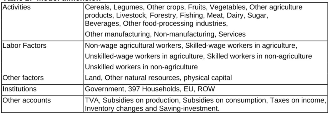
(13) Model Disaggregation Table 2 displays the disaggregation of activities, factors and institutions. The model comprises 17 activities, 14 of which are agriculture and food processing. Table 2: Model dimension Activities. Cereals, Legumes, Other crops, Fruits, Vegetables, Other agriculture products, Livestock, Forestry, Fishing, Meat, Dairy, Sugar, Beverages, Other food-processing industries, Other manufacturing, Non-manufacturing, Services. Labor Factors. Non-wage agricultural workers, Skilled-wage workers in agriculture, Unskilled-wage workers in agriculture, Skilled workers in non-agriculture Unskilled workers in non-agriculture. Other factors. Land, Other natural resources, physical capital. Institutions. Government, 397 Households, EU, ROW. Other accounts. TVA, Subsidies on production, Subsidies on consumption, Taxes on income, Inventory changes and Saving-investment.. All activities use capital and labor. Each agricultural activity requires land (except livestock). Non-manufacturing activities dominated by extraction and mining use an additional factor representing the change in the level of extraction of natural resources: oil, gas, phosphates etc. The current model desegregation allows each activity to produce only one commodity. The model includes 397 households representing the Tunisian population and based on a sample of representative households extracted from the 1995 survey on household expenditures in Tunisia. The other institutions are the government and the ROW, which is divided into the EU and non-EU, given that one purpose of the analysis is to evaluate the impact on poverty from Tunisia’s partnership agreement with the EU. Model Structure The following section is not intended to describe precisely the characteristics of the model employed here, but rather to describe in non-mathematical terms its main hypotheses and the developments introduced on its basic structure for the requirement of this study. A formal presentation of this model is available in Beghin, Dessus, Roland Holst and Van Der Mensbrugghe (1996) Prices are endogenous on each market (goods, factors) and equalize supply and demand so as to obtain the equilibrium. The equilibrium is general in the sense that it concerns all the markets simultaneously. Supply is modeled using nested constant elasticity of substitution (CES) functions, which describe the substitution and complementary relations among the various inputs. Producers are cost-minimizers and constant return to scale is assumed. Output results form a combination of two composite goods in fixed proportions: intermediate consumption and value added. The intermediate aggregate is obtained by combining all products in fixed proportions (Leontief structure). The value-added is then 13.
(14) decomposed into two substitutable parts: labor and capital. Capital is further disaggregated between the different categories using a CES function (physical capital, natural resources, and land). Since the main focus of this study is to evaluate the impact of trade policy reform on poverty, the labor factor is further disaggregated into five categories according to the sector of employment (i.e. agricultural activities versus non-agricultural activities) and skill level (i.e. skilled versus un-skilled). A fifth type of labor, specific to the agricultural sector, was added to the four categories listed above. It represents the familial work or the unpaid work performed by the farmers and their family members in the agriculture sector. The relative wage by worker is estimated using the sectoral remuneration of each category (as it appears in the Social Accounting Matrix, SAM) on one side and the total number of workers by category and sector on the other. Accordingly, this version of the model has been extended from its original structure to better account for the potential substitutability between unskilled labor engaged in agricultural and non-agricultural sectors. In particular, the model features a nested structure of the production function, which allows for high substitutability between unskilled workers in agricultural sectors and unskilled workers in non-agricultural activities. Only at the upper nest of the production function are the respective aggregates (unskilled workers in all activities) merged with skilled labor and family workers. This more flexible functional form guarantees a more realistic substitutability between factors that are close substitutes and avoids excessive substitution of factors that are complementary to each other. Thus, family workers are considered specific to agricultural activities and are fully employed. A flexible wage is applied for this segment, which assures the equilibrium between supply and demand. For skilled workers, it is assumed that they are specific for both types of activities (agricultural versus non-agricultural). Both skilled and unskilled workers are supposed to be remunerated at constant real wage levels. Accordingly, the model assumes the existence of unemployment for both skilled and unskilled workers in agricultural as well as non-agricultural activities. Income from labor and capital is allocated to the different households according to a fixed coefficient derived from the SAM. Household demand is derived from maximizing the utility function, subject to the constraints of available income and the consumer price vector. Household utility is a positive function of consumption of the various products and savings. Income elasticities are differentiated by product and household, and vary from 0.75 for staple products of households with highest income to 1.20 for services. The calibration of the model determines a per capita subsistence minimum for each product and each household, which will be consumed whatever the price and the income of the households, while the remaining demand is derived through an optimization process. The subsistence share in the 14.
(15) consumption of basic goods is higher than the share in the consumption of luxury goods. Government and investment demands are disaggregated in sectoral demands once their total value is determined according to fixed coefficient functions. The model assumes imperfect substitution among goods originating from different geographical areas (the so-called Armington assumption). Import demand results from a CES aggregation function of domestic and imported goods. Export supply is symmetrically modeled as a constant elasticity of transformation function. Producers decide to allocate their output to domestic or foreign markets responding to relative prices. At the second stage, importers (exporters) choose the optimal choice of demand (supply) across regions, again as a function of the relative import (export) prices and the degree of substitution across regions. Substitution elasticity between domestic and imported products is set at 2.2, and at 5.0 between imported products according to origin (EU or ROW). The elasticity of transformation between products intended for the domestic market and products for export is 5.0, and 8.0 between the different destinations for export products.6 Several macro-economic constraints are introduced in this model. First, the small country assumption holds, given that the Tunisian economy is unable to change world prices. Thus, its import and export prices are exogenous. Capital transfers are exogenous as well, and therefore the trade balance is fixed, so as to achieve the balance of payments equilibrium. Second, the model imposes a fixed real government deficit and fixed real public expenditures. Public receipts thus adjust endogenously in order to achieve the predetermined net government position by shifting the Value Added Tax (VAT) rate. Third, investment is determined by the availability of savings, the latter originating from households, government, and abroad. Since government and foreign savings are exogenous in this model, changes in investment volumes reflect changes in household savings and changes in the price of investment. Policy impacts are compared to the situation observed in 1996, in terms of macroeconomic indicators, sectoral performance, and poverty indicators. Even though the model is static, it captures the long term re-allocation effects of different trade policies, since adjustment costs of reallocating productive factors are ignored. However, it does not incorporate the dynamic effects of trade policies, and notably their impact on GDP growth, since resources (labor, capital, and productivity) are fixed in this model. Interpretations of results are therefore to be taken with caution, since they only indicate what would be the impact of a given policy on the allocation of resources, and not on their levels.. 6. Production function and trade elasticities come from the empirical literature devoted to CGE models. They are not specific to Tunisia. See for instance Burniaux, Nicoletti, and Martins (1992), Konan and Maskus (1997) or more recently Gallaway, McDaniel and Rivera (2000). 15.
(16) Database A disaggregated SAM for 1996 has been constructed and used to calibrate the model parameters. Data were collected from various sources and the SAM building process had been done in several steps. In the first step, a Micro SAM that had the same account disaggregation than the original Input-Output table published by the INS (2000b) had been constructed. It includes a total of 19 activities where agriculture and food processing industries are aggregated in two separate accounts. It also includes only two production factors (labor and capital) and three institutions (a representative household, government, and the ROW). In the second step, the agriculture and food processing activities have been broken down into several sub-activities. The disaggregation takes into account a mapping carried out between production sectors and major groups of commodities consumed by households. Accordingly, the single agricultural activity was disaggregated into six subactivities, along with the food processing activity. The other activities (17) were aggregated into two residual sectors: other manufacturing, and services. Technical standards describing input requirements of the various agricultural activities (Ministère de l’Agriculture, 1993) were used in the disaggregation of the agricultural sector. A matrix of input shares by activity is then derived and used to disaggregate the original agricultural activity into the six different sub-activities. Data on output value as well as on input prices are based on official estimates (Ministère de l’Agriculture, 1997)7. In a third step, labor as well as capital accounts were disaggregated, the labor account into five categories and the physical capital into three types. For the agricultural sector, the equivalent wage for non-wage workers in the agricultural sector is estimated using the total number of working days by the agricultural activities obtained from the 1995 Farms Structure Survey (Ministère de l’Agriculture, 1996) and remunerated at current wages for skilled and unskilled workers. For this purpose, it is assumed that farmers are skilled while family members are unskilled. The remuneration of the land factor is approximated using the observed rental rate on the market and the allocated surfaces by activity. The corresponding amounts for remuneration of non-wage workers as well as land are deduced from the total remuneration of capital as it appears in the original IO table and added individually into the SAM. In addition, the wage-workers for all sectors are further disaggregated into skilled and unskilled workers using data from the INS (1999). Lastly, the ROW account is further disaggregated into two accounts: the EU and the non-EU countries. Data on trade as well as on transfers between domestic institutions and. 7. More details on the disaggregation of agriculture and production factors are found in Chemingui and Dessus (1999). 16.
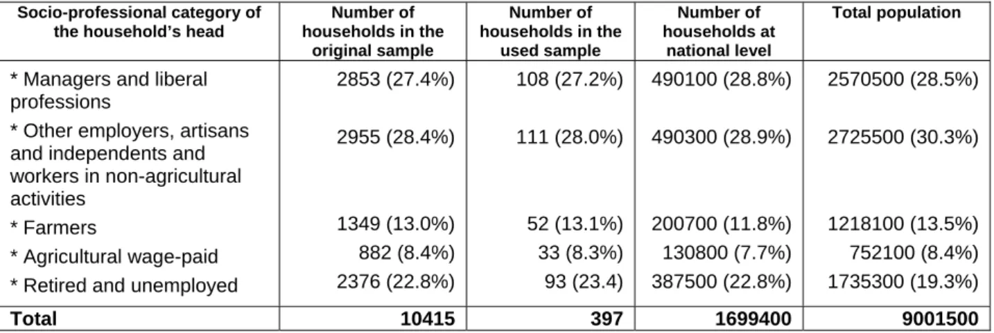
(17) foreign partners are based on the INS (1999). For trade protection, it is assumed that Tunisia applies the same tariff structure for all trade partners. The MicroSAM represents in itself a first step in data preparation for a microsimulated CGE model. Thus, a SAM fully integrating a micro-module is required for the purpose of this study. This micro-module should cover both income and expenditures for all households included in the sample. In Tunisia, the household survey provides only quantitative data on the structure of expenditure by major commodities for each single household. However, information on the structure as well as the level of income by household is limited to the sector or the professional status of the head of the household. Accordingly, the first task in building the micro-module is the estimation of the level of income by household as well as its source. Alternative methods are used for the estimation of the micro-module. The estimation of the income side for the households’ sample is justified by two major reasons. Firstly, even static analyses of poverty can be carried out using data on detailed consumption expenditures; proceeding to prospective analyses cannot be fulfilled in the absence of data on sources and levels of households’ incomes. Secondly, variations in the level of poverty in a specific country are the twin result of prices changes (relative to consumer goods) and income changes, as a consequence of variations in wage levels and rents. Limiting poverty analysis to the consumption side omits an important channel in the analysis, which is the change of income levels. The original sample provided by INS contains 400 households extracted from the 1995 household expenditures survey. This sample is expected to be representative of the whole sample of 10,415 Households surveyed in 1995. The first step in building the micromodule consists of checking the representativeness of the sample with the whole survey’s sample. To do so and for additional reasons of simplification, the professional statuses of the household’s heads, classified originally by the INS into 12 categories, are mapped only with 5 major categories. Then, an estimation of the shares of households in the survey’s sample having one of the five professional statuses has been made and applied to the available sample. To be consistent with the survey, three households are dropped from the available sample. Table 3 provides details on the repartition of the total surveyed households and the used sample according to the above classification of households by professional status.. 17.
(18) Table 3: Representativeness of the sample by socio-professional category of the household's head in 1995 Socio-professional category of the household’s head. * Managers and liberal professions * Other employers, artisans and independents and workers in non-agricultural activities * Farmers * Agricultural wage-paid * Retired and unemployed. Number of households in the original sample. Number of households in the used sample. Number of households at national level. Total population. 2853 (27.4%). 108 (27.2%). 490100 (28.8%). 2570500 (28.5%). 2955 (28.4%). 111 (28.0%). 490300 (28.9%). 2725500 (30.3%). 1349 (13.0%) 882 (8.4%) 2376 (22.8%). 52 (13.1%) 33 (8.3%) 93 (23.4). 200700 (11.8%) 130800 (7.7%) 387500 (22.8%). 1218100 (13.5%) 752100 (8.4%) 1735300 (19.3%). 10415. 397. 1699400. 9001500. Total. Source: Author’s calculations based on INS data Note: In parentheses, the percentage from the total of every column. For the income estimation purpose, it is assumed that the distribution of the total expenditure by household in the sample is a proxy of income distribution, which means that total household revenue equals the total expenses. While this assumption omits the fact that many households generate a surplus of saving and others are rather indebted, it does not influence the results too much since the used model represents a real economy and does not take into account its financial aspects. However, a homogeneous saving rate is applied afterwards when balancing the SAM. Once total income by household of the sample is estimated, the question of how to determine its sources remains. The qualitative data on the professional status of the members of the household allow the drawing out of a table on the sources of income by household’s member and then by household. The next step consists of the estimation of the level of income by source and by household’s member. For this purpose, three main sources of income are considered: wages, rents, and transfers. Given that wages represent the main source of income for the majority of Tunisian households, the results of the employment survey conducted annually by the INS were used for the estimation of the levels of wages received by each household member. These levels of wages relative to the years 1996 and 1997 (INS, 1999) are established by professional category and economic activity. However, and for independent workers who do not receive a salary, an equivalent-salary is then estimated. It equates the salary level provided by the same activity to a wageworker with the same level of qualification. For a simplification of the estimation process, only poor households are assumed to receive transfers both from the government in the form of aid or from abroad in the form of remittances. Furthermore, it is assumed that poor households do not receive rents in the form of return to investment or factor remuneration (land).. 18.
(19) For the independent workers, two categories are identified. The poor households characterized by a level of income lower than the poverty line, and the non-poor households having a level of income above the poverty line. For each household in the sample, wages as well as capital income and rents received are differentiated by economic activity wherein the members of the household are working either as wage earners or as independent workers. The difference between the wages (or equivalent wages) and the total income of each household represents the transfers to poor households, while the income generated from the other factors (capital and land) goes to non-poor households. Land remuneration is estimated using the corresponding market value of rent for the year 1996. The last adjustment performed on the micro-module consists of multiplying both income and expenditure for each household in the sample by the corresponding weight of the corresponding category of household in the total Tunisian population. The last step in the data preparation is the full integration of the micro-module in the SAM. When the micro-module is imposed on the 1996 SAM table (assuming otherwise unchanged column coefficients) most of the accounts are out of balance, as expected. In order to eliminate these imbalances, the cross-entropy model8 was applied. In this application, the model minimized cross entropy subject to (i) equality between column and row totals for the disaggregated household accounts; (ii) a set of constraints without errors that impose equality between a) the sum of payments between disaggregated households and any non-household account and b) as control values, the corresponding payments between the single household and other accounts in the preceding balanced matrix; and (iii) a set of constraints with errors that impose control values based on exogenous estimates for the share of each household in total household consumption. 5.. Simulations To assess the policy effects of trade reforms on macro-economic aggregates, trade. volumes, sectoral outputs, and poverty indicators are compared with those in the reference scenario. Given that the model used in this study is static, the economy is not affected by structural modifications, as demography or the changes in the levels of availability of land and other natural resources are, for example. Four scenarios are analyzed here. The first experiment (L1) consists of evaluating the effect of phasing-out tariffs on manufactured products imported from the EU. The second experiment (L2) looks at the effects of tariff liberalization on all imports from the EU, including agricultural products. The 8. Cross entropy is a technique for solving underdetermined estimation problems that has been applied to the estimation of IO tables (Golan, Judge and Robinson, 1994) and social accounting matrices (Robinson, Cattaneo and El -Said, 2001) as well as a wide range of other problems inside and outside economics. For a detailed presentation of the cross entropy model applied for SAM balancing, see Robinson, Cattaneo and El -Said (2001) and Lofgren, Chemingui and El-Said (2004). 19.
(20) third scenario (L3) extends tariff dismantling on imports from the non-EU countries. Finally, the fourth experiment (L4) combines the effects of unilateral liberalization as specified in the third scenario with a multilateral agricultural liberalization. The latter is reflected by the expected rise in world prices of most agricultural and food products imported by Tunisia as an outcome of a multilateral agreement on agricultural trade under the Doha Round. While this tool does not takes into account dynamical effects that will intervene during the liberalization process, it nevertheless presents the advantage of allowing the measurement of the total gain related to the reallocation of production factors as a result of trade liberalization. The results of the four scenarios are presented in tables 4-8. They indicate deviations from the base values, showing the impact of each of the four scenarios described above. For poverty, four indicators are computed. The headcount ratio (P0) measures the proportion of the population that is poor using the selected poverty line (lower poverty line defined by the World Bank, 2003)9. The second indicator is the number of poor. The relevance of this indicator can be explained by the fact that in some cases, a decline in poverty incidence with an increase in the number of poor is observed. The poverty gap (P1) and the squared poverty gap (P2) represent the third and the fourth indicators of poverty measures. The poverty gap ratio indicates the extent to which individuals fall below the poverty line as a proportion of the poverty line. The sum of these poverty gaps calculated with respect to Tunisia’s poverty line would give the cost of eliminating poverty if transfers were perfectly targeted. The square poverty gap averages the squares of the poverty gaps relative to the poverty line, putting more weight on the poorest sectors. It represents a measure of how poor the poor are. For the measure of inequality, the most popular indicator is the Gini coefficient, which ranges from 0 (perfect equality) to 1 (perfect inequality).. 9. The lower poverty line adopted by the World Bank for 1995 was 196 TD at the national level, which corresponds to 483 PPP US$. It implies a lower urban poverty line of 218 TD (537 PPP US$) and a rural lower poverty line of 185 TD (456 PPP US$) 20.
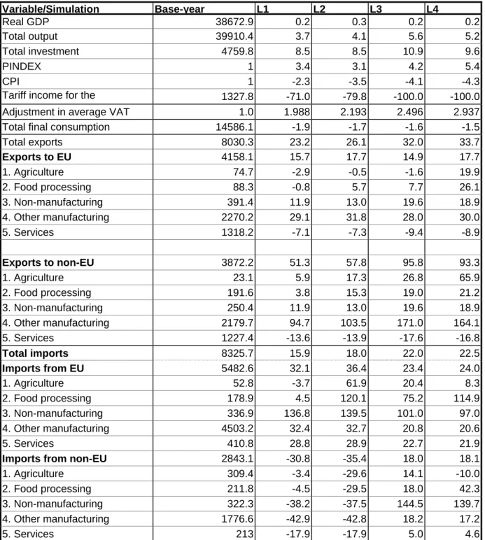
(21) Table 4: Macroeconomic results Variable/Simulation Real GDP Total output Total investment PINDEX CPI Tariff income for the Adjustmenttin average VAT Total final consumption Total exports Exports to EU 1. Agriculture 2. Food processing 3. Non-manufacturing 4. Other manufacturing 5. Services. Base-year. L1 38672.9 39910.4 4759.8 1 1 1327.8 1.0 14586.1 8030.3 4158.1 74.7 88.3 391.4 2270.2 1318.2. L2 0.2 3.7 8.5 3.4 -2.3 -71.0 1.988 -1.9 23.2 15.7 -2.9 -0.8 11.9 29.1 -7.1. L3 0.3 4.1 8.5 3.1 -3.5 -79.8 2.193 -1.7 26.1 17.7 -0.5 5.7 13.0 31.8 -7.3. L4 0.2 5.6 10.9 4.2 -4.1 -100.0 2.496 -1.6 32.0 14.9 -1.6 7.7 19.6 28.0 -9.4. 0.2 5.2 9.6 5.4 -4.3 -100.0 2.937 -1.5 33.7 17.7 19.9 26.1 18.9 30.0 -8.9. 3872.2 51.3 57.8 95.8 93.3 Exports to non-EU 1. Agriculture 23.1 5.9 17.3 26.8 65.9 2. Food processing 191.6 3.8 15.3 19.0 21.2 3. Non-manufacturing 250.4 11.9 13.0 19.6 18.9 4. Other manufacturing 2179.7 94.7 103.5 171.0 164.1 5. Services 1227.4 -13.6 -13.9 -17.6 -16.8 8325.7 15.9 18.0 22.0 22.5 Total imports 5482.6 32.1 36.4 23.4 24.0 Imports from EU 1. Agriculture 52.8 -3.7 61.9 20.4 8.3 2. Food processing 178.9 4.5 120.1 75.2 114.9 3. Non-manufacturing 336.9 136.8 139.5 101.0 97.0 4. Other manufacturing 4503.2 32.4 32.7 20.8 20.6 5. Services 410.8 28.8 28.9 22.7 21.9 2843.1 -30.8 -35.4 18.0 18.1 Imports from non-EU 1. Agriculture 309.4 -3.4 -29.6 14.1 -10.0 2. Food processing 211.8 -4.5 -29.5 18.0 42.3 3. Non-manufacturing 322.3 -38.2 -37.5 144.5 139.7 4. Other manufacturing 1776.6 -42.9 -42.8 18.2 17.2 5. Services 213 -17.9 -17.9 5.0 4.6 Source: Author’s calculations Note: Values in the base-year are expressed in millions Tunisian Dinar (TD). For alternative scenarios, values represent percentage change compared to the base-year. Data are rounded to one decimal point.. 21.
(22) Table 5: Sectoral production (in percentage change compared to the base-year) Base-year L1 L2 L3 L4 Variable/Simulation Cereals 590.9 -0.5 -0.1 -1.8 -1.8 Legumes 32.5 -1.8 -0.8 -0.1 -5.5 Other crops 220.4 -1.6 -8.7 -9.9 35.0 Fruits 840.2 -0.7 -0.6 -0.8 0.5 Vegetables 526.4 -0.9 0.0 0.0 -5.6 Other agricultural activities 29.1 7.5 4.3 6.9 -2.4 Livestock 1011 -3.2 -6.7 -7.7 -2.7 Forestry 72.3 -1.2 -1.4 -1.5 -1.8 Fishing 276.3 -6.4 -6.6 -8.6 -9.6 Meat 633.1 -4.1 -8.2 -8.7 -3.5 Milk 191.3 0.1 -14.7 -20.4 8.4 Sugar 141.2 -1.3 -2.9 -6.6 64.0 Beverages 227.9 -4.0 -7.6 -7.7 -3.1 Other food processing activities 2765 -1.5 0.1 0.7 -12.6 Other manufacturing 11404 16.4 18.3 23.6 23.5 Non-manufacturing industries 2362 8.7 9.7 15.9 14.4 Services 18587 -0.9 -0.9 -0.8 -1.3 Source: Author’s calculations Note: values in the base-year are expressed in millions TD. For alternative scenarios, values represent percentage change compared to the base-year.. Table 6: Sectoral exports Base-year L1 L2 L3 L4 Variable/Simulation Cereals 1.5 20.8 47.1 78.4 149.5 Legumes 1.9 5.7 20.0 28.6 107.1 Other crops 1.0 13.9 41.8 54.1 1121.1 Fruits 57.1 3.2 5.4 6.2 8.7 Vegetables 5.8 11.2 22.7 25.3 -0.2 Other agricultural activities 3.0 18.2 28.6 39.0 -2.4 Livestock 6.2 -5.3 0.6 2.6 19.7 Forestry 0.0 0.0 0.0 0.0 0.0 Fishing 21.3 -19.8 -20.2 -27.5 -25.9 Meat 1.6 -8.5 -2.8 -2.8 318.3 Milk 1.8 12.5 17.5 21.3 908.8 Sugar 3.6 3.2 14.5 14.0 1650.0 Beverages 16.9 1.6 3.3 4.7 11.2 Other food processing activities 271.3 0.8 9.5 12.2 9.4 Other manufacturing 4449.9 42.0 45.9 56.1 56.3 Non-manufacturing industries 641.8 11.9 13.0 19.6 18.9 Services 2545.6 -8.2 -8.4 -10.8 -10.2 Source: Author’s calculations Note: values in the base-year are expressed in millions TD. For alternative scenarios, values represent percentage change compared to the base-year.. 22.
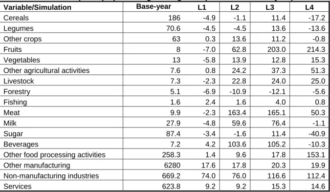
(23) Table 7: Sectoral imports (in percentage change compared to the base-year) Base-year Variable/Simulation L1 L2 L3 L4 Cereals 186 -4.9 -1.1 11.4 -17.2 Legumes 70.6 -4.5 -4.5 13.6 -13.6 Other crops 63 0.3 13.6 11.2 -0.8 Fruits 8 -7.0 62.8 203.0 214.3 Vegetables 13 -5.8 13.9 12.8 15.3 Other agricultural activities 7.6 0.8 24.2 37.3 51.3 Livestock 7.3 -2.3 22.8 24.0 25.0 Forestry 5.1 -6.9 -10.9 -12.1 -5.6 Fishing 1.6 2.4 1.6 4.0 0.8 Meat 9.9 -2.3 163.4 165.1 50.3 Milk 27.9 -4.8 59.6 76.4 -1.1 Sugar 87.4 -3.4 -1.6 11.4 -40.9 Beverages 7.2 4.2 103.6 105.2 -10.3 Other food processing activities 258.3 1.4 9.6 17.8 153.1 Other manufacturing 6280 17.6 17.8 20.3 19.9 Non-manufacturing industries 669.2 74.0 76.0 116.6 112.4 Services 623.8 9.2 9.2 15.3 14.6 Source: Author’s calculations Note: values in the base-year are expressed in millions TD. For alternative scenarios, values represent percentage change compared to the base-year.. Table 8: Effects on poverty Base. L1. L2. L3. L4. Poverty incidence (P0) National 8.1 7.7 7.7 7.6 Urban areas 3.2 3.5 3.5 3.5 Rural areas 15.8 14.3 14.3 14.1 Number of poor National 735215 -4.7 -4.9 -5.7 Urban 178005 10.3 9.8 9.8 Rural 557210 -9.5 -9.5 -10.6 Poverty gap index (P1) National 1.72 1.83 1.83 1.82 Urban areas 0.36 0.34 0.34 0.34 Rural areas 3.55 3.92 3.91 3.91 Severity of poverty (P2) National 0.59 0.58 0.58 0.58 Urban areas 0.11 0.11 0.11 0.11 Rural areas 1.24 1.19 1.19 1.19 Gini coefficient National 0.417 0.415 0.409 0.394 Urban areas 0.389 0.39 0.385 0.371 Rural areas 0.353 0.345 0.357 0.342 Source: Authors’ calculations Notes: P0, P1, and P2 are calculated at the lower poverty line according to the World approach (2003). Number of poor in the base-year is expressed in persons. In the alternative scenarios, represent percentage change compared to the base-year. 5.4 3.7 7.9 -33.7 16.4 -49.7 1.82 0.27 4.15 0.58 0.12 1.16 0.424 0.401 0.38 Bank's figures. 23.
(24) Results for the four scenarios show a relatively small improvement in economic activity with an increase in GDP ranging between 0.2 and 0.3 percentage points compared to the base year. However, the amplitude of gains is higher on total output and trade. In this respect, the first scenario induces a 3.7 percentage point increase in the total output compared to 4.1, 5.6 and 5.2 respectively for the second, the third and the fourth scenarios. For the first three scenarios (L1, L2 and L3), the increase of total output is mostly driven by the activities with relatively lower levels of value added which are mostly in the manufacturing sector, such as textiles and clothing. However, for the forth scenario (L4), the contribution of the agricultural and food sectors in the growth of total production is illustrated by the improvement in the level of domestic production for other crops, milk, and sugar, and a lower decrease for the other activities. In addition, the lower domestic prices for imported goods in all scenarios, except for some agricultural products in the fourth scenario, are illustrated by a decline in the consumer price index, which explains the drop in the real value of final consumption. The loss of tariff income is offset by an increase in the average rate of VAT, which rises proportionally with the amplitude of trade liberalization. In the first scenario (L1), the rate is increased by 1.988 times than the base-year, moving from an average of 4.2 percent to 8.34 percent. However, the rate of VAT reached 9.21 percent, 10.48 percent and 12.33 percent respectively for the second, the third and the fourth scenarios. The changes in trade are the most important net effects of the various simulations. Due to the preference granted by Tunisia to European industrial products, imports from the Rest of the World experience a high decline compared to the base-year with a decrease of about one third. However, imports from the European Union experience an increase by approximately the same level as the decline of the Rest of the World’s share in the Tunisian market. In the first scenario (L1), the increase in exports is largely due to the expansion of the industrial sector, whereas agricultural exports tend to fall in volume. Gains in competitiveness allowing Tunisia to increase its export market share are not due to genuine depreciation, given that the price of value added remains unchanged, because the cut in revenue on capital offsets the rise in real wages. These gains are in fact due to the reduction in prices of imported inputs and a lessening of the distortion of international trade other than in agriculture, a situation, which benefits the industrial sector particularly. Agricultural activity does not appear to be able to derive benefit from the increasing openness of the Tunisian economy to trade and partnership with Europe, and remains to a large extent outside the globalization process. Moreover, mobile production factors (physical capital and unskilled labor) are more captured by industry, which is translated into a drop in domestic production for most of agricultural activities as a result of changes in comparative advantage to the 24.
(25) benefit of industrial sector. Accordingly, consumer prices for agricultural products climb and those for industrial products fall, leading to a change in poverty patterns for both categories of household. Naturally, the changes in poverty are also explained by the changes in wage levels and other factors’ income (physical capital and land). In this respect, relative real wages for skilled workers in agricultural activities as well as farmers decline in the first stage. However, the resulting higher wages in the non-agricultural sector increase the level of mobility of wage-workers from agricultural activities to non-agricultural activities, which in turn increases real wages in rural areas. Consequently, and combined with lower consumer prices, the welfare of the Tunisian population as a whole goes up and poverty declines. However, there is a net increase of poverty in urban areas as a result of lower real wages. The reinforcement of the European Union’s preferential status on the Tunisian market has a very-weak macro-economic impact compared to the previous simulation (L1). In fact, the inclusion of agricultural products in the agreement is reflected in a marginal rise in total import volume (2% compared with the first simulation). All of these new imports come from Europe. Consequently, the volume of imports from the Rest of the World declines, but proportionally less than the rise in imports from Europe. In other words, consumers substitute European imports for imports from the Rest of the World and local production given that domestic production for almost all products declined. The loss in customs income is evaluated at around 79.8 percent of total government customs income in 1996. Only 8.8 percent of this loss can be attributed to the liberalization of trade in agricultural products. The total level of production increase closely marginally by an additional 0.4 percentage points in volume compared to its level before this reform. The higher increase was realized by the same sectors as in the previous simulation, which included other food processing activities, other manufacturing, and non-manufacturing industries. For the rest of agricultural and food processing activities, we observe an improvement in the levels of domestic production for cereals, legumes, other crops, fruits, vegetables, and other agricultural activities, given that the decline in their domestic production is lower than in the previous simulation (L1). However, for the rest of agricultural and food activities (livestock, forestry, fishing, meat, milk, sugar, and beverages), the decline in domestic production is higher than in the first scenario. This is the direct effect of the loss in competitiveness of domestic products compared to the European products being highly subsidized. For these same sectors, a higher increase in imports is observed. The decline in the domestic prices for these imported products increases the profitability of the existing capital in these activities and allows a reallocation of the primary production factors from the weakly integrated activities that participate in international trade to the activities which benefit most from trade openness. 25.
(26) Compared to the first scenario, this reform (L2) does not remain unchanged with respect to the incidence of poverty in both urban and rural areas. However, there is a slight decrease in the number of poor in urban areas directly linked to lower domestic prices for some agricultural products, mainly those structurally imported by Tunisia. For the Gini coefficient it goes from 0.417 to 0.409, implying that changes in trade policy have a positive impact on income distribution for the whole population. However, income distribution is only improved for urban households, while it is negative for rural households. For all households, the simulation L2 reduces the domestic prices of both agricultural and manufacturing products. Producers gain from the decrease in input and equipment prices, while consumers gain from lower consumption prices. However, the effect of this reform on urban households is more mitigated. In fact, the decrease in the number of poor has only affected the households, where the heads are employed as wageworkers in the non-agricultural sectors, as a result of higher real wages. This decrease is the direct result of the relative development of certain urban activities, mainly those which maintain an unskilled workforce (for which the country has a comparative advantage such as textiles and clothing) and which are enjoying a lower cost for their imported equipment. However, farmers and agricultural workers benefit less from tariff liberalization on all imports from the European Union given the relatively low dependence of the agriculture sector on imported goods on one side and the comparative advantage of European products on foreign markets as a result of the support provided by the Common Agricultural Policy, on the other. The generalization of tariff dismantling on imported agricultural products (L3) causes an improvement in the global activity of the country by 5.6 percent in comparison with the base-year and 1.5 percentage point compared to the second simulation (L2). Total exports as well as total imports increase in comparison with the base-year respectively by 32 percent and 22 percent, which means an additional increase by 5.9 percent for exports and 4 percent for imports in comparison with the L2 simulation. The increase in exports is mainly explained by the increase in the demand for Tunisian products by the Rest of the World in comparison with the base-year. At the sectoral level, this reform entails a fall in the domestic production of most agricultural activities. This decrease is explained by the weak capacity of the Tunisian agricultural sector in resource reallocation. In other words, the agricultural land, suitable for cultivation in Tunisia is characterized by an almost fixed distribution of its productive capacities. If, for example, the production price of cereal products rises, in comparison with vegetables, the assignment of the available land from the cultivation of vegetables towards cereal production is too limited, even impossible. Accordingly, the. 26.
(27) adjustments in Tunisian agriculture are more the result of changes in the consumption levels than the production levels, in reaction to changes in the relative prices. The effect of this reform on poverty is a consolidation of the observed tendencies in the preceding scenario. Thus, the farmers’ incomes are improved, especially because of the improvement in the preferences given to Tunisian agriculture by the Rest of the World, and the decrease in the costs of agricultural input. This mostly concerns the price of seeds and cattle food. The improvement in the profitability of some agricultural activities prompted wages to increase. These combined result in a very small decline in poverty incidence for the country (-0.1 percentage point). This reduction in poverty incidence is explained by a significant decline in the number of poor in rural areas, which compensate for the increase in the number of poor in the urban areas. In addition, this reform increases income distribution both at the national as well at regional levels. The fall in the Gini coefficient is homogeneous across areas. Along with the three previous scenarios, the last scenario (L4) simulates an increase in the world prices of the basic agricultural products as a result of a multilateral liberalization of trade in agricultural products. The analysis of the implications of agricultural trade liberalization at the country level must not be limited to the mere removal of tariff and nontariff barriers, imposed on imported products. Through trade, the trade balance situation of agricultural products, for such a small country as Tunisia is largely determined by world prices, mostly the result of policies implemented in rich countries exporting agricultural products. Nefarious and undesirable effects of high agricultural protectionism in the rich countries exporting basic agricultural products have remained through the decades. On the one hand, protection has depressed the agricultural world prices, which, in fact, has penalized all farmers by shrinking the world market. On the other hand, protection has caused much greater instability in world prices, which led all countries into a vicious cycle of protection. A potential conclusion of the Doha round, according to the ministerial declaration of Hong Kong, could appreciably affect the world market in basic agricultural products, and considerably reduce the distortions that have affected it for so long. Thus, we simulate here an increase in the world prices of the basic agricultural products, resulting from a scenario of thoroughly freed world agricultural trade and the removal of all the distortions that affect them. The expected changes in world prices as a result of multilateral agricultural liberalization under the DDA used in this study are based on the estimation carried out by Bchir, Ben Hammouda, Chemingui and Karingi (2007). During the simulation period, the changes are expected to vary between 1.75 percent and 23 percent compared to the baseyear. The total production of goods and services rises by 5.2 percent compared with the base 27.
(28) year; a net reduction of 0.4 percent compared with the L3 scenario. Total imports as much as total exports rise respectively by 22.5 percent and 33.7 percent compared with the baseyear. The scenario L4 thus enhances the competitiveness of domestic agricultural production for three categories of products: other crops, milk, and sugar, which witness a net increase in their production. This shock also includes a rise in the consumption prices of the main agricultural products, which consequently implies the reduction of the internal demand for these products. Thus, the reduction of production on one hand, and the relatively high decrease in the consumption of the main food products on the other hand, leads to an increase in export levels as a net result of the rise in export prices. This situation was actually observed during the previous agricultural year (2005) in Tunisia for olive oil, when the high level of export prices led to a rise in consumption prices, which weakened the level of local demand and consequently increased the level of exports. This scenario, consequently gives a favorable income gain to agricultural households who attain a higher level of income following the rise in world prices, while urban households witness a deterioration of their purchasing power following the rise in the consumption prices of most agricultural products. As far as poverty is concerned, this scenario leads to a high reduction in the poverty level (poverty rate drops from 8.1% to 5.4% compared with the base-year). However, the reduction in poverty incidence is higher for rural households (from 15.8 to only 7.9%) following the generalized increase in agricultural wages and farmers’ income. Accordingly, the number of poor in rural areas decreases by almost half its level in the base-year while the number of urban poor increase by more than 16 percent. Finally, this simulation improves income distribution for rural households but deteriorates for urban households. 6.. Conclusion Tunisia has carried out a number of reforms in the frame of its structural adjustment. program, but the level of agricultural protection remains one of the highest in the world. At the same time, and like many countries in the Arab world, Tunisia is a net agricultural importer. Its main exports are olives and dates, and the principle imports are wheat and maize. Multilateral liberalization is expected to raise agricultural prices. If all agricultural commodity prices rise proportionately, Tunisia will face declining terms of trade because it is a net agricultural importer. On the other hand, it would benefit from domestic liberalization due to efficiency gains. The combined effect is likely to be positive for Tunisia as a whole because most estimates show that efficiency gains are larger than terms-of-trade losses. However, the combination of global and domestic liberalization would probably reduce agricultural prices because the effect of the loss in high levels of protection (89% on average) 28.
Figure
+3

Related documents