Optimal tax progressivity in unionised labour markets : simulation results for Germany

(1)

Dis cus si on Paper No. 10-035

Optimal Tax Progressivity in

Unionised Labour Markets:

Simulation Results for Germany

(2)

Dis cus si on Paper No. 10-035

Optimal Tax Progressivity in

Unionised Labour Markets:

Simulation Results for Germany

Stefan Boeters

Die Dis cus si on Pape rs die nen einer mög lichst schnel len Ver brei tung von neue ren For schungs arbei ten des ZEW. Die Bei trä ge lie gen in allei ni ger Ver ant wor tung

der Auto ren und stel len nicht not wen di ger wei se die Mei nung des ZEW dar.

Dis cus si on Papers are inten ded to make results of ZEW research prompt ly avai la ble to other Download this ZEW Discussion Paper from our ftp server:

(3)

Non-technical summary

What is the optimal degree of income tax progressivity when both labour supply and wages are endogenous, and households are heterogeneous in several dimensions? This question is answered using a numerical combined micro-macro model. The micro part features approximately 4600 individual households with varying wages and labour supply reactions. The macro part includes sectoral collective wage bargaining and involuntary unemployment. Thus the fundamental trade-o created by increasing tax progressivity is captured. On the one hand, higher marginal tax rates distort individual labour supply. On the other hand, higher tax progressivity has a wage-moderating and unemployment-reducing eect under collective wage bargaining.

In this general setting, varying tax progressivity is implemented as a stepwise one-percentage-point increase of the marginal wage income tax and a compensating transfer to all working individuals, which keeps the public budget balanced. The most important simulation results are the following:

• A welfare maximum is reached at a point where marginal income tax rates are

six percentage points above the initial level.

• The welfare gain at this point averages a moderate two euros per household

and per month.

• This average welfare gain is overshadowed by considerable redistributive

ef-fects, which range from a loss of more than 300 euros to a gain of almost 200 euros.

• Labour supply eects of higher tax progressivity are positive at the

participa-tion margin and negative at the hours-of-work margin. The net eect varies by skill group; it is positive for the low skilled, but negative for the medium and high skilled.

• At the same time higher tax progressivity reduces the unemployment rate. This

eect dominates, so that overall labour input to production (in wage-weighted hours of work) increases.

• Higher labour supply elasticities lead to a lower optimal degree of tax

progres-sivity. More elastic wage curves or more elastic international capital supply work in the opposite direction.

(4)

Nicht-technische Zusammenfassung

Wie hoch ist der optimale Grad der Steuerprogression, wenn Arbeitsangebot und Löhne endogen sind und sich Haushalte in mehreren Dimensionen unterscheiden? Diese Frage wird mittels eines gekoppelten, numerischen Mikro-Makro-Modells be-antwortet. Im Mikro-Modul bildet das Modell rund 4600 Haushalte mit unterschied-lichen Löhnen und Arbeitsangebotsreaktionen ab. Im Makro-Modul nden sich sek-torale kollektive Lohnverhandlungen und unfreiwillige Arbeitslosigkeit. So kann der fundamentale Zielkonikt bei der Bestimmung der Steuerprogression erfasst werden. Einerseits verzerren hohe marginale Steuersätze das individuelle Arbeitsangebot. Andererseits wirkt Steuerprogression bei kollektiven Lohnverhandlungen lohnsen-kend und vermindert so die Arbeitslosigkeit.

In diesem Modellrahmen wird Steuerprogression als eine stufenweise Erhöhung der marginalen Lohnsteuer abgebildet, wobei steuerzahlende Individuen mit einer Anpassung des Freibetrags so kompensiert werden, dass das öentliche Budget aus-geglichen bleibt. Dabei ergeben sich die folgenden Simulationsergebnisse:

• Das Wohlfahrtsmaximum wird an einem Punkt erreicht, wo die marginalen

Steuersätze um sechs Prozentpunkte höher liegen als im Ausgangszustand.

• Der Wohlfahrtsgewinn beträgt dann im Mittel bescheidene 2 Euro pro

Haus-halt und Monat.

• Der mittlere Wohlfahrtsgewinn wird überschattet von erheblichen

individuel-len Umverteilungseekten, die von einem Verlust von mehr als 300 Euro bis zu einem Gewinn von 200 Euro reichen.

• Die Arbeitsangebotseekte höherer Steuerprogression sind positiv in Bezug

auf Partizipation und negativ in Bezug auf die Anzahl Arbeitsstunden. Der Nettoeekt variiert je nach Qualikationsgruppe: positiv für die Geringquali-zierten, negativ für die Mittel- und Hochqualizierten.

• Gleichzeitig reduziert Steuerprogression die Arbeitslosenquote. Dieser Eekt

dominiert den Arbeitsangebotseekt, so dass die makroökonomische Beschäf-tigung (in lohngewichteteten Stunden) steigt.

• Höhere Arbeitsangebotselastizitäten haben einen geringere optimale

Steuer-progression zur Folge. Elastischere Lohnkurven und höhere internationale Ka-pitalmobilität wirken in die entgegengesetzte Richtung.

(5)

Optimal Tax Progressivity in Unionised Labour

Markets: Simulation Results for Germany

Stefan Boeters

∗

CPB, Netherlands Bureau for Economic Policy Analysis, Den Haag ZEW, Centre for European Economic Research, Mannheim

May 2010

Abstract

Changing the income tax progressivity in labour markets with collective wage bargaining generates a trade-o. On the one hand, higher progressivity distorts individual labour supply decisions at the hours-of-work margin, on the other hand, it reduces unemployment by exerting downward pressure on wages. This trade-o is quantitatively assessed using a numerical model for Germany. The model combines a microsimulation module, which captures the labour-supply decisions of approximately 4600 individual households, and a macro (compu-table general equilibrium) module, which features collective wage bargaining and involuntary unemployment.

In the simulations carried out using this model, the optimal degree of tax progressivity turns out to be higher than the one in the actual German tax schedule. The optimum is located at marginal tax rates that are 6 percentage points higher than the actual rates (combined with a transfer that balances the public budget). The welfare gain from such a reform is modest, however. It amounts to no more than two euros per person per month.

Keywords: labour taxation, tax progressivity, optimal taxation, collective wage bargaining, unemployment, microsimulation, computable general equi-librium model

JEL Code: C63, C68, H21, J22, J51, J64

∗_{Stefan Boeters, CPB, P.O. Box 80510, NL-2508 GM Den Haag, e-mail: [email protected].}

I thank Markus Clauss, Egbert Jongen and Holger Stichnoth for helpful comments on earlier versions of this paper.

(6)

1 Introduction

When we analyse the economic eects of income tax progressivity, obtaining a full picture is only possible if we take account of three dierent eects. First, tax pro-gressivity is a means of redistribution, because average tax rates are higher for the rich than for the poor. Second, the higher the marginal tax rates, the higher the distortionary eects on individual labour supply decisions. Third, tax progressivity changes the conditions for collective wage bargaining and aects the level of wages and unemployment. In this paper I present an applied simulation model for Ger-many, which allows for an integrated analysis of these eects possible and enables us to derive the optimal degree of tax progressivity.

In the policy debate, the redistributive eect of income tax progressivity is clearly dominating. Economists have traditionally emphasised the eciency aspect. A high degree of tax progressivity means high marginal tax rates at the upper end of the income distribution. This leads to large labour supply distortions in the high-income group and, as a consequence, decreases the overall scope for redistribution. Mirrlees (1971) was the rst to derive criteria for an optimal tax schedule, which balances redistributive and distortionary eects (see Tuomala (1990) for a comprehensive overview of the literature based on the Mirrlees approach). When translating these criteria into a realistically quantied tax schedule we are, however, confronted with three major problems. (1) Labour supply is not only exible at the hours-of-work margin, but also at the participation margin (this has been addressed by Saez, 2002). (2) The income tax system covers households of varying composition, which leads to incommensurable utility functions. (3) Individuals are not only heterogeneous with respect to their earnings potential (as assumed by Mirrlees), but also with respect to their leisure preferences, which also makes them dicult to compare.

These complications have led to the evolution of a second approach, which takes household heterogeneity seriously in several dimensions and is less concerned with the derivation of analytic optimality conditions. This approach is rooted in the tradition of econometric labour supply estimation and microsimulation (Fortin et al., 1993; Aaberge and Colombino, 2008; Ericson and Floot, 2009). The increase in complexity caused by introducing exible functional forms for the estimation of utility functions comes at the expense of exibility in the tax schedule. Rather than

(7)

deriving local marginal optimality conditions (as in Mirrlees, 1971), the search for an optimal system is restricted to a relatively small set of free parameters (e.g. stepwise constant marginal tax rates). Bourguignon and Spadaro (2005) can be placed in this tradition as well. They invert the problem, however, and ask which social welfare function would produce the existing tax schedule as an optimal choice.

Both approaches described above remain within a partial labour market frame-work: wages are xed and there is no involuntary unemployment. Since the 1980s, however, extensive research into non-competitive labour markets has shown that tax progressivity has important eects on wage formation as well(Hersoug, 1984; Lockwood and Manning, 1993; Holmlund and Kolm, 1995; Koskela and Vilmunen, 1996). Tax progressivity lowers the incentives for high wage claims and leads to a downward pressure on non-competitive wages, which in turn reduces involuntary unemployment.

Few attempts have been made to quantify the trade-o between the positive eect of tax progressivity on wage formation and its negative eect on labour sup-ply (Holmlund and Kolm, 1995; Sørensen, 1999; Boeters, 2009). These attempts remain within an aggregate representative-agent approach and do not combine non-competitive wage formation and the heterogeneity of individual households. This is where the present paper comes into play. I use a consistent micro-macro simulation set-up developed during the past few years (Böhringer et al. (2005); Arntz et al. (2008); Boeters and Feil (2009)). In the microsimulation part, the model features a discrete labour supply choice, where the parameters of the utility function are estimated along the lines of van Soest (1995). The computable general equilibrium (CGE) part features sectoral wage bargaining between trade unions and employers' organisations, which results in wages that are above the market-clearing level, and thus leads to involuntary unemployment.

In this paper I use this micro-macro set-up to determine optimal tax progressi-vity. Performing counterfactual experiments with systematically varying tax sche-dules, I nd an optimal tax schedule with marginal tax rates that are a few percen-tage points higher than the ones in the initial situation. This benchmark optimum is determined without any welfare weighting, according to the Kaldor-Hicks criterion of potential compensation of the losers. Adding redistributive motives to the social welfare function would drive the results towards even higher tax progressivity.

(8)

The simulations also show that the welfare function is relatively at around the optimum. The welfare gain of a switch from the initial to the optimal point is no more than 2 euros per person per month. In addition, the maximum point reacts sensitively to assumptions about core parameters. In the sensitivity analysis it is shown that the level of optimal tax progressivity is increased by a lower elasticity of labour supply, by higher wage curve elasticity and by higher international capital mobility.

The plan for the rest of the paper is as follows. In Section 2, the two modules of the model micro and macro and their linkage are presented. Section 3 describes the welfare calculations and Section 4 the scenarios to be implemented. Section 5 presents the main simulation results, followed by Section 6 with the sensitivity analysis. Section 7 summarises and concludes. The appendix contains details of the labour supply estimation that underlie the microsimulation module.

2 Simulation set-up

The model used in this paper to perform a numerical analysis of tax progressivity is based on an integrated micro-macro set-up. The micro part of the model consists of a discrete choice (DC) labour supply module with heterogeneous households. The macro part is a multi-sectoral computable general equilibrium (CGE) model of an open economy with collective wage bargaining. The two parts are rst presented separately in Sections 2.1 and 2.2. In Section 2.3, I turn to the micro-macro linkage and describe how consistent feedback loops are constructed. Arntz et al. (2008) provides a more extensive discussion of the linked model.

2.1 Microsimulation of labour supply

At the basis of the labour supply module is the microsimulation model for Germany by Buslei and Steiner (1999). This model combines a household income calculator under the current German tax and transfer system and a DC labour supply estima-tion of the van Soest (1995) type. Discrete labour supply opestima-tions (which combine the respective amounts of income and leisure) for all households are constructed

(9)

using information from the German Socio-Economic Panel, GSOEP (see Table 3 in the appendix).

In the DC setup, the utility of labour-supply option k for household j of type i

is a combination of a deterministic part,_{U ,}¯ _{which depends on a vector of individual}

and alternative-specic characteristics, xj,k, and an additive stochastic error term,

εj,k:

Ui(xj,k) = ¯Ui(xj,k) +εj,k.

The distinctive feature of the logit approach is that the error term is assumed to be independently standard extreme-value distributed. This makes it possible to derive

an explicit formula for the probability of preferring option k over all other options

l 6=k from a setm (McFadden, 1974):

P(Ui(xj,k)> Ui(xj,l)) =

exp( ¯Ui(xj,k)) P

mexp( ¯Ui(xj,m))

, ∀l 6=k

Following van Soest (1995), the utility function_U¯_i _{is specied as a translog function}

with coecients Ai and βi, which capture the quadratic and linear terms

respecti-vely:

¯

Ui(xj,k) = x0j,kAixj,k +βi0xj,k.

Each option is characterised by the logs of disposable income and weekly hours of leisure for men and women:

xj,k = (log(Ci(hfj,k, h m j,k)),log(T −h f j,k),log(T −h m j,k)),

where hf _and _hm _{are the working hours of the spouses and} _T _{is time endowment.}

The coecients Ai and βi include interactions between leisure, income and a

num-ber of household characteristics. Fixed costs of working are captured by constant terms for specic labour-supply options. The coecients are estimated separately for couples, female singles and male singles from a sample of approximately 4600 GSOEP individuals (see Table 4 in Appendix A.1). A complete list of regressors and the detailed estimation results can be found in Appendix A.2.

Given the estimation results, simulation of a counterfactual situation proceeds along the lines of Duncan and Weeks (1998) and Creedy and Kalb (2005). Random numbers are drawn from the extreme-value distribution, and only those consistent

(10)

with the actual choice of the respective household are retained. In the subsequent si-mulation, with changed disposable incomes for the individual labour supply options, the optimal choice will change for a subset of these random numbers. In the initial situation, each household chooses exactly one option, whereas in the post-reform situation, we may end up with a genuine probability distribution over all options.

2.2 The CGE framework

The labour supply module is embedded in a computable general equilibrium model of Germany (PACE-L). In this section, the main parts of the model are briey sketched. An extensive, algebraic model description and a summary of the data

sources used for calibration can be found in Böhringer et al. (2005).1

Private households

The model comprises three representative worker households, each representing the aggregate labour supply of one skill type in the microsimulation module. This co-vers all households with exible time allocation and observable hours of work, which constitute roughly 60% of total labour supply. The rest is captured by one residual worker household with xed labour supply. Finally, there is a separate capitalist household, which receives all capital income and decides on consumption and in-vestment according to the approach of Ballard et al. (1985). The utility function of the capitalist household is calibrated to empirical saving elasticities. Worker hou-seholds, in contrast, do not save. The structure of consumption is assumed to be identical across all households.

Firms

In each of seven aggregate production sectors, a representative rm produces a homogeneous output. The production functions are of the nested constant-elasticity-of-substitution (CES) type, combining intermediate inputs, capital and labour of the three skill types. For the value-added nest, we adopt the NNCES approach of Perroni

(11)

and Rutherford (1995), which allows us to calibrate labour demand elasticities to

the set of estimated cross-price eects in Falk and Koebel (1997).2 _{Each individual}

rm is assumed to be small in relation to its respective sector. All rms in one sector interact through monopolistic competition, so that rms can exploit market power in their individual market segment. Cost minimisation yields demand functions for the primary factors of production and intermediate demand at the sectoral level. Capital is mobile across sectors, and the domestic market for capital is perfectly competitive. International capital mobility is imperfect. (See Section 6.3 for a sensitivity analysis with respect to international capital supply.)

Wage formation

In the largest part of the labour market, i.e. the low- and medium-skilled segments, wages are determined by sector- and skill-group-specic negotiations between em-ployers' associations and trade unions. The bargaining outcome is generated through the maximisation of a Nash function, which includes the objective functions of both parties and their respective fallback options. In the model, the right to manage ap-proach is adopted: Parties bargain over wages, and rms determine labour demand on the basis of the bargained wage. The objective function of the trade unions is of the insider type: value of a job minus value of the outside option. The latter in turn is composed of two components, associated with the chances of nding a job in another sector or remaining unemployed. The values of labour market states are determined as weighted averages of incomes in the case of employment and unem-ployment, where weights are computed from the probabilities of transition between employment and unemployment (see Pissarides, 1990, for an overview of the search-and-matching approach). Collective wage bargaining results in wages that are above the market-clearing level, with involuntary unemployment as the consequence.

In contrast to the low- and medium-skilled segments, the high-skilled labour market is assumed to be competitive, and there is no involuntary unemployment. Accounting for unemployment, the three labour markets are balanced by aggrega-ting, on the demand side, over sectors and, on the supply side, over households of

2_{The extension of the model to three skill groups with NNCES calibration is described in Boeters}

(12)

the respective skill type. With respect to other household characteristics apart from the skill type, it is assumed that the structure of labour demand is uniform across sectors.

Government

The main focus of the model is on the complex tax and transfer system for private households, whose budget constraints are calculated in the microsimulation module (see Section 2.1). Apart from labour income taxes, the government collects uni-form capital input taxes, prot taxes, output taxes in production and dierentiated consumption taxes. The government budget encompasses the revenue from all these taxes, transfers to private households, the public purchases of goods, and the ba-lance of payments surplus or decit. In the policy simulations (see Section 4), the level of public consumption is kept constant and the transfers to private households are adjusted to ensure that the public budget is in balance.

Foreign Trade

According to the small-open-economy assumption, export and import prices in fo-reign currency are not aected by the domestic economy. International trade is modelled adopting the Armington (1969) assumption of product heterogeneity by market of origin and destination. Domestically produced goods are converted into specic goods destined for the domestic market and the export market through a constant-elasticity-of-transformation function. Analogously, a CES function charac-terises the choice between imported and domestically produced varieties of the same good. The output of this CES aggregation is used both as intermediate and nal demand. Foreign closure of the model is warranted through the balance-of-payments constraint.

2.3 Linking the microsimulation and CGE modules

If we had a closed-form formula for individual labour supply, it would in principle be possible to integrate all equations of the two modules in a single model and try to

(13)

solve it simultaneously. However, as labour supply is simulated with random numbers (see Section 2.1), the modules must be kept separate and iterated until they produce a consistent solution. In the policy simulations (Section 5) I start with the modied rules of the tax and transfer system and rst simulate labour supply changes under the assumption of constant wages and unemployment rates. The resulting labour supply is aggregated by skill type and transferred to the CGE module, which is then solved under the assumption of a xed labour supply. This results in changes in wages, unemployment rates and transfers to balance the public budget. These variables are fed back to the labour supply module for the next iteration. This is continued until the two modules converge.

When linking the wage bargaining equations to the microsimulation module, it is assumed that all individual households (of the respective skill group) are uniformly represented by the trade union. Marginal tax rates and the values of employment and unemployment are calculated as (hours-weighted) averages over all households and labour supply options. In turn, the wages and unemployment rates that result in the CGE module are used to derive the income positions of all employed or unemployed households.

3 Welfare calculations

In previous applications (e.g. Boeters and Feil, 2009), the micro-macro model has been used only for a descriptive analysis, i.e. for tracing out the consequences of policy changes for observable economic variables, without any sort of welfare as-sessment. For the present analysis, the model needs to be extended with a welfare module. For this purpose, I draw on the work of Creedy and Kalb (2005), adjusted for the fact that utility of the households is conceptualised as an expected value.

It has been shown in Section 2.1 that the utility function is translog with

house-hold consumption and leisure as arguments. Expected utility, EU, of labour supply

optionkfor householdj of typeiis the probability-weighted (pi,n) sum over the

uti-lities in the dierent labour market states n (employed/unemployed, i.e. two states

for singles, four for couples):

EUj,k = X

n

pi,n

ai,C(log(Cj,k,n))2+ ˜βi,Clog(Cj,k,n) +Rj,k

(14)

In contrast to Section 2.1, 1 focuses only on the terms related to household

consump-tion. ai,C is the coecient of the quadratic log-consumption term, β˜i,C is the

coef-cient that collects all terms that are linear in log-consumption (including the

in-teraction terms with leisure), and Rj,k is a residual collecting all terms that do not

depend on consumption at all.

In a discrete choice setting, the calculation of the Hicksian equivalent variation

(EV) is complicated by the fact that we do not know beforehand which

labour-supply option the household will choose. In the initial situation, householdj chooses

option k, providing utility level EUj,k. In the counterfactual situation simulated, it

chooses l, providing utility level EU¯ j,l. However, neitherk nor l need be the option

it would choose if it were compensated lump-sum (the ction underlying the EV

calculation) instead of undergoing the actual policy change. Therefore EV must be

calculated for all possible options (indexm). This is done using the following implicit

formula for EV: ¯ EUj,l = X n pi,n

ai,C(log(Ci,j,n+EVi,m,n))

2

+ ˜βi,Clog(Ci,j,n+EVi,m,n) +Ri,j

Under normal circumstances, option-specicEV will be constant across labour

mar-ket states (EVi,m,n =EVi,m, ∀n). However, a complication arises because for some

households,EV can be negative and larger (in absolute terms) than their

consump-tion in the case of unemployment. This would make the log funcconsump-tion undened. To

avoid this case, I set a lower bound on EVi,m,n, which is slightly above −Ci,j,n, and

allowEVi,m,n to deviate from the other options if it is at its lower bound.3

Individual equivalent variation is the minimum of the option-specic values (Creedy and Kalb, 2005):

EVj = min

m (EVj,m)

Finally, the change in total welfare is calculated by summing up all individualEVs.

We can restrict ourselves to the individuals in the micro module, because all other agents are compensated so that their welfare remains constant (see Section 4).

EV =X

j

EVj

3_{In these cases the non-restricted value of} _EV

i,m,n is selected for the welfare calculations. As

(15)

By taking the unweighted sum of theEVs as welfare measure, I adopt the

Kaldor-Hicks criterion of potential compensation. If total EV is positive, the winners of

the tax reform could compensate the losers. The principal caveat of this criterion is that as long as no actual compensation takes place, distributional aspects do matter, but are not accounted for. It would be desirable to apply some distributional

weigh-ting to the EV changes, at least as a sensitivity analysis. However, this runs into

the problem that the utility functions are inherently incommensurable, because the parameters vary by household. Therefore, no straightforward basis for weighting is available. Aaberge and Colombino (2008) propose a weighting method that involves two diverging utility functions per household. I do not adopt this approach in the present paper because of the consistency problems implied.

4 Scenario denition

In the micro module of the linked model, the budget constraint is characterised for each household by the average burden and one or two marginal burdens (for single and couple households respectively) per labour-supply option. These burdens summarise the complete tax and transfer system, they comprise the income tax, social security contributions and, possibly, transfer payments. In the simulations, the conditions (though not the incidence) of the latter are kept xed and the income tax schedule is varied.

According to the German income tax schedule, the marginal tax rate is increasing in taxable income, with two dierent slope parameters up to a certain threshold income, and constant thereafter. The average tax rate is monotonously increasing in taxable income as well, asymptotically approaching the highest marginal tax rate for very high incomes (see Figure 1).

In the simulations, I gradually increase the progressivity of the tax schedule. The marginal tax rate is raised by the same number of percentage points everywhere (shift from initial to scenario in Figure 1). To compensate the increase in tax income that would result from an isolated increase in the marginal tax rates, I introduce a uniform transfer paid to each working individual. These two changes are combined to a new average tax schedule, which is rst below, then above the initial

(16)

Figure 1: German income tax schedule (2005) -0.2 -0.1 0 0.1 0.2 0.3 0.4 0.5 0 20000 40000 60000 80000 100000 120000 Tax rate

Taxable income (euros per year) marginal tax, intitial

average tax, intitial

marginal tax, scenario average tax, scenario

one. Figure 1 shows the case of a 6 percentage-points increase of the marginal tax rates as scenario. This is the change that turns out to be optimal in the base case simulations of Section 5. In this scenario, the budget-balancing transfer amounts to 1416 euros per year (118 euros per month). With this transfer in place, the reform is favourable for single households with a taxable income of below 30,000 euros,

whereas households with a higher income lose.4

The welfare assessment in the scenarios is slightly complicated by the fact that the worker households with exible labour supply are not the only households in the model (see Section 2.2, households). The residual worker household and the capitalist household are also aected by the reform, through changing wages and returns to capital respectively. As utility functions that allow us to evaluate wel-fare changes are only dened for households in the microsimulation module, further adjustment parameters are introduced to restrict welfare changes to this group. Lump-sum transfers are adjusted in order to keep real income of the residual hou-seholds is kept precisely at its initial value. When evaluating welfare changes, we

4_{Here I assume that earnings do not change. They do change in the model, where wages are}

(17)

Figure 2: Welfare eects of varying tax progressivity 0 0.1 0.2 0.3 0.4 0.5 0.6 0.7 0 2 4 6 8 10 12

Welfare change (aggregate EV in bln. euros)

Increase in marginal tax on labour (percentage points)

1000 random error terms 100 random error terms

can then focus on the households in the microsimulation module when evaluating welfare changes.

5 Simulation results

The simulation set-up described in Section 4 produces welfare eects that are concave in tax progressivity. Welfare is maximised at marginal tax rates that are 6 percentage points above the initial level. Figure 2 shows the welfare prole, Figure 1 (scenario) the tax schedule at the maximum point.

Figure 2 also illustrates that a relatively large number of random numbers is necessary to produce a smooth shape of the curve. Curves with 100 random error terms per individual (broken lines) show a lot of non-concave segments and are vola-tile. Only with 1000 random numbers (the average of the 10 cases with 100 numbers shown in bold), is the curve suciently smooth for a single, global maximum to be discerned. Even in the case of 1000 random numbers, perfect convexity is not reached yet, and we had better describe the welfare maximum as being somewhere between a 5- and an 8-percentage-point increase of the marginal tax rates.

(18)

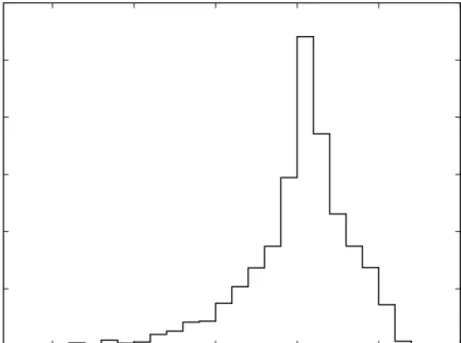
Figure 3: Distribution of welfare eects across households 0 0.002 0.004 0.006 0.008 0.01 0.012 -300 -200 -100 0 100 200 Density

EV in euros per month

The aggregate equivalent variation (EV) reached in this region is

approxima-tely 500 million euros per year. Given that the microsimulation module represents roughly 21 million people, this amounts to 24 euros per person per year, or 2 euros per month. This is a small amount compared to the redistribution that is taking place at the same time. Figure 3 shows the distribution of the welfare eects across households at the maximum point (where marginal tax rates are 6 percentage points

higher). There is a large variation with EV ranging from a loss of more than 300

euros to a gain of almost 200 euros. The distribution is skewed, the tail with the losses is thicker, and the median is at approximately 18 euros, considerably more than the average of 2 euros.

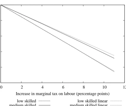
Is it possible to identify the model mechanisms that are responsible for the average welfare gain on top of all the redistribution that is taking place? Let us look at a number of model outcomes in order to get a feeling for what drives the results. To begin with, Figure 4 shows the changes in labour supply (total hours, i.e. both at the intensive and extensive margin).

The labour supply eects dier qualitatively across skill groups. For the low skilled, labour supply increases with the degree of tax progressivity, for the medium

(19)

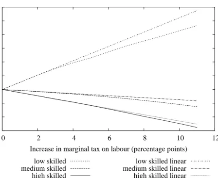
Figure 4: Labour supply by skill group -1.5 -1 -0.5 0 0.5 1 1.5 2 2.5 3 0 2 4 6 8 10 12

Labour supply, both margins (change in %)

high skilled medium skilled low skilled

high skilled linear medium skilled linear low skilled linear

skilled it decreases slightly, for the high skilled considerably so. The reaction of each skill group is almost linear. For comparison the curves with the addition linear extrapolate the eect of the rst percentage point change linearly. For all skill groups the deviation from the linear curve is negative, i.e. with high progressivity there is a more than linear disincentive to work. We will see that this is the driving force behind the results; but to obtain a clear picture, we continue our analysis of the results.

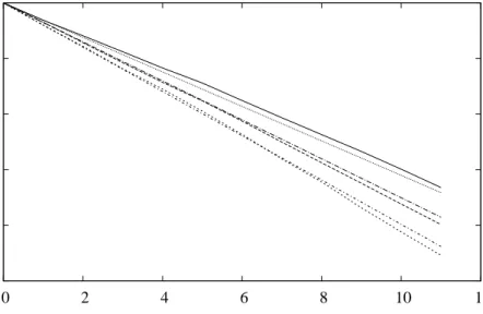
Next, we break the labour supply eects down into changes along the hours-of-work and the participation margins (Figures 5 and 6). Hours of hours-of-work decrease for all skill groups, the dierences between skill groups are small and the deviations from the linear responses are not uniform. Participation increases for all groups, the dierences among groups are considerably larger than for hours of work, and the deviations from the linear schedule are always negative. For the low skilled, the participation eect dominates the hours-of-work eect, whereas the latter do-minates for the two other skill groups. The participation eect is largest for the low skilled because in this group, participation is lowest from the start, hence there are considerably more indiviuals left who can be activated by higher labour supply incentives.

(20)

Figure 5: Hours-of-work eects by skill group -2.5 -2 -1.5 -1 -0.5 0 0 2 4 6 8 10 12

Hours of work (change in %)

Figure 6: Participation eects by skill group

0 0.5 1 1.5 2 2.5 3 3.5 0 2 4 6 8 10 12

Participation rate (change in %-points)

(21)

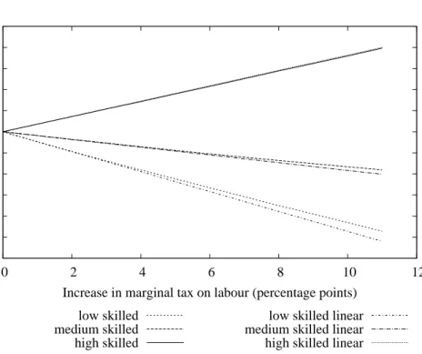
Figure 7: Wage changes by skill group -6 -5 -4 -3 -2 -1 0 1 2 3 4 5 0 2 4 6 8 10 12 Wage (change in %)

Next, we take a look at wages and unemployment rates. Figure 7 shows the change in skill-specic wages. The wage reaction to tax progressivity is characteris-tically dierent depending on the skill group. The wages of the high skilled increases, whereas the medium skilled and particularly the low skilled suer a wage drop. It is not possible to infer the causal direction of the interaction between the labour market variables from a simple inspection of the gures. However, the skill-specic wage reactions may be interpreted as a consequence of the changes in labour supply (Figure 4), which are attenuated, but not reversed, by the wage changes.

Figure 8 shows unemployment for the medium and low skilled. (The high skilled are fully employed by assumption). The gure reveals that the unemployment reac-tion is almost linear and almost proporreac-tional to initial unemployment rates. Since for the low skilled the initial unemployment rate (22 %) is far higher than for the medium skilled (7 %), unemployment changes, when measured in percentage points, are highest in this segment as well.

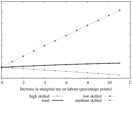
Finally, we turn to total labour input to production. Given that we have changes both in labour supply and unemployment which is the overall eect on labour input (in wage-weighted hours)? Of particular interest are the medium skilled (the

(22)

Figure 8: Unemployment by skill group 0.75 0.8 0.85 0.9 0.95 1 0 2 4 6 8 10 12

Unemployment, relative to initial level

Increase in marginal tax on labour (percentage points) medium skilled

low skilled

medium skilled linear low skilled linear

largest group), where both labour supply and unemployment are decreasing, so that the overall eect is unclear. Figure 9 shows that the net eect for the medium skilled is positive and slightly increasing in tax progressivity. Labour input of the low skilled increases considerably, whereas it falls for the high skilled. A wage-weighted average of all labour-input changes (bold line total) almost precisely coincides with the curve for the medium skilled, with an increase that remains below half a per cent.

Figure 10 shows the transfer that is paid to compensate the wage income re-cipients for the higher marginal wage tax (so that the public budget is kept in balance). This transfer increases almost linearly with the change of the marginal tax rate to more than 200 euros per month. As a benchmark, a linear extrapolation of the change at the rst one per cent increase is depicted in Figure 10 as Transfer (li-near). The actual transfer is slightly less than linear, and it turns out to be exactly this deviation that leads to the welfare maximum in the model. At an 11-percentage-point increase of the marginal tax rate, the deviation from the linear development is approximately 5 euros per month, in the region of the welfare maximum, it is approximately 1 euro per month.

(23)

Figure 9: Total labour input (weighted hours) -1 0 1 2 3 4 5 6 0 2 4 6 8 10 12

Employment, relative to initial level

Increase in marginal tax on labour (percentage points) total

high skilled

medium skilled low skilled

Figure 10: Lump-sum transfer to balance public budget

0 50 100 150 200 250 0 2 4 6 8 10 12

Transfer per individual (in euros/month)

(24)

How is it possible to proceed from the observation of non-linear model reactions to the identication of the driving forces? In order to nd out the causal direc-tion of the eects, I run a number of diagnostic scenarios. First, I implement the line Transfer (linear) from Figure 10 as a scenario, i.e. I compensate individuals with the linear extrapolation of the rst incremental transfer, neglecting the bud-get constraint. In this simulation the welfare maximum disappears (at least within the region covered), and, instead, welfare increases monotonously with tax progres-sivity. This identies the non-linearity in the transfer as a crucial element in the determination of the welfare maximum.

What then is the cause of the non-linearity in the transfer? The next identica-tion step is to check whether the initial impulse comes from the micro or the macro part of the model. The second diagnostic scenario therefore consists in linearising the macro module, by feeding the linear reactions of wages (Figure 7) and unemploy-ment (Figure 8) back into the micro module. This does not eliminate the non-linear reactions of labour supply (Figure 4). In contrast, when I linearise the micro module and feed linear reactions in labour supply (Figures 5 and 6) back into the macro module, the non-linearities in wages and transfers almost entirely disappear. This identies the micro module as the source of the initial eect.

With regard to the labour supply reactions produced by the micro module (Fi-gures 5 and 6), we have already found participation (Fi(Fi-gures 6) to be the dominating factor. How can we explain that participation while increasing monotonously for all skill groups increases less than linearly? The reason lies in the probability distribu-tion assumed in the logit labour supply model. The individual, unobservable utility components of the dierent labour supply options here we focus on the option non-participation are extreme-value distributed. The extreme-value distribution is, similar to the normal distribution, single-peaked, and its density decreases the greater the distance from zero. Small changes in the attractiveness of one labour supply option will thus have a larger eect when they are close to the initial si-tuation (at zero) than when they are farther away. This is the non-linearity that eventually drives the results.

(25)

6 Sensitivity analysis

In the sensitivity analysis of the results, I vary the basic model set-up in three places: elasticity of labour supply, elasticity of the wage curve with respect to tax progressivity, and international capital mobility. The rst two of these variations are backed up with straightforward economic intuitions. When labour supply becomes more elastic, we expect the welfare loss through labour supply distortions to increase and thus tax progressivity to become less attractive. Conversely, when the wage curve reacts more sensitively to higher tax progressivity, the contribution of tax progressivity to reducing labour market distortions resulting from collective wage bargaining is more signicant, and tax progressivity becomes more attractive. In Sections 6.1 and 6.2 I investigate whether the model results conrm these intuitions, and what this means in quantitative terms. In Section 6.3, I turn to the degree of international capital mobility, which has proved to be an important driving force of the results in earlier applications of PACE-L (see Boeters and Feil, 2009). In this case, we have no a priori expectation about the direction of the eect, however.

6.1 Variation in labour supply elasticities

The elasticity of labour supply is an obvious candidate for sensitivity analysis, be-cause it governs the distortions in labour supply, which constitute one side of the trade-o we are exploring. However, the elasticity of labour supply is not a single parameter in the model that could easily be varied. Rather, it results from the in-teraction of all individual parameters in the utility functions, which determine the relative attractiveness of leisure versus consumption. None of these parameters can easily be singled out for variation.

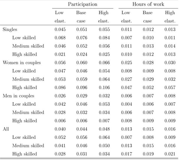
As a practical solution, I vary all parameters that are connected with leisure in the utility functions (linear, quadratic and interaction terms with other variables) with the same multiplier. It turns out that this almost exactly translates into pro-portional changes of labour supply elasticities. A multiplier of 0.9 leads to approxi-mately 10 % lower labour supply elasticities (columns Low elast. in Table 1), a

(26)

Table 1: Labour supply elasticities

Participation Hours of work

Low Base High Low Base High elast. case elast. elast. case elast. Singles 0.045 0.051 0.055 0.011 0.012 0.013 Low skilled 0.068 0.076 0.084 0.007 0.010 0.011 Medium skilled 0.046 0.052 0.056 0.011 0.013 0.014 High skilled 0.021 0.024 0.025 0.010 0.012 0.013 Women in couples 0.056 0.060 0.066 0.025 0.028 0.030 Low skilled 0.047 0.046 0.054 0.008 0.009 0.008 Medium skilled 0.053 0.059 0.064 0.027 0.029 0.032 High skilled 0.086 0.096 0.106 0.047 0.052 0.057 Men in couples 0.026 0.029 0.032 0.006 0.007 0.008 Low skilled 0.042 0.046 0.053 0.004 0.006 0.007 Medium skilled 0.028 0.032 0.034 0.006 0.007 0.008 High skilled 0.006 0.006 0.007 0.008 0.009 0.009 All 0.040 0.044 0.048 0.013 0.015 0.016 Low skilled 0.052 0.056 0.064 0.007 0.008 0.009 Medium skilled 0.041 0.046 0.050 0.013 0.015 0.016 High skilled 0.028 0.031 0.034 0.017 0.019 0.021

multiplier of 1.1 to elasticities that are 10 % higher than in the base case (columns

High elast.).5

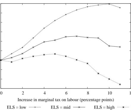
Figure 11 shows the welfare eects. As expected, the lower labour supply elas-ticities, the higher welfare gains from higher tax progressivity, with corresponding shifts of the welfare maximum. When labour supply elasticities are low, maximum welfare is reached at marginal tax rates that are 10 percentage points higher than

5_{Labour supply elasticities have been simulated by increasing all gross wages simultaneously}

by 10% and then aggregating over individual discrete reactions. Interaction eects are very small, thus this yields almost the same results as varying wages separately group by group.

(27)

Figure 11: Varying labour supply elasticity: welfare -0.6 -0.4 -0.2 0 0.2 0.4 0.6 0.8 1 1.2 0 2 4 6 8 10 12

ELS = low ELS = mid ELS = high

in the initial situation, when elasticities are high, the maximum is at tax rates that

are 5 percentage points higher.6

Figures 12 and 13 show the actions of the underlying labour market variables. For the largest group, the medium skilled, eects are clear-cut. With higher labour supply elasticity, the negative labour supply eects of the base case are amplied, which leads to a higher wage. For the low and high skilled (which are considerably smaller groups), the patterns are less clear-cut. There is hardly any change in low skilled labour supply and high skilled wages, due to interaction eects with the other skill groups.

In the sensitivity analysis, labour supply elasticities have only been varied in

a narrow range (±10 %), less than the variation that can be found in empirical

estimates. This restriction was deliberate, since I wanted to keep the welfare maxi-mum in the range covered by the simulations of the base case. Further simulations conrmed what can be expected by extrapolating from Figure 11. If labour supply

6_{The calculations in the sensitivity analysis are based on simulations with 100 sets of random}

error terms. For this purpose, a set is chosen that produces aggregate results similar to the extended 1000-error-terms set in Section 5. Nevertheless, curve ELS = mid in Figure 11 does not exactly coincide with the one in Figure 2.

(28)

Figure 12: Varying labour supply elasticity: labour supply -2 -1.5 -1 -0.5 0 0.5 1 1.5 2 2.5 3 0 2 4 6 8 10 12 Wage (change in %)

Increase in marginal tax on labour (percentage points) low skilled

medium skilled

high skilled

ELS = low ELS = mid ELS = high

Figure 13: Varying labour supply elasticity: wage

-6 -5 -4 -3 -2 -1 0 1 2 3 4 5 0 2 4 6 8 10 12 Wage (change in %)

Increase in marginal tax on labour (percentage points) low skilled medium skilled high skilled

(29)

elasticities are even lower, then the welfare eect is monotonously increasing over the full range of marginal tax rates, if they are higher, the curve is monotonously decreasing.

6.2 Variation in wage curve elasticities

Similar to the case of labour supply elasticities, we can make an informed guess about what would happen if the wage bargaining system (represented by wage curves) reacted more or less sensitively to a variation of tax progressivity. As the positive eect of tax progressivity is reducing unemployment by exerting downward pressure on wages, the welfare eects of tax progressivity are expected to be the more positive, the more sensitively the wages react.

However, again similar to the case of labour supply elasticities, there is no free parameter in the model that directly governs the responsiveness of the wage to variations in tax progressivity (or other institutional parameters). The latter is the result of the integrated wage bargaining system, whose only parameter, the relative bargaining power of the trade unions, has been xed in the calibration so that the actual level of unemployment is met. There is no other parameter that could be varied to systematically modify the responsiveness of the wage bargaining system to changes in labour market conditions.

In this sensitivity analysis, I use a modelling shortcut and make the bargaining strength parameter a linear function of tax progressivity. In the high elasticity (EWC = high) scenario, bargaining strength of the trade union decreases in tax progressivity, so that the wage drops more than in the base case with a constant bargaining parameter (and vice versa for the low elasticity scenario). The linear parameter is chosen so that in the high (low) elasticity scenario the responsiveness of the wage curve to tax progressivity is 25 % higher (lower) than in the base case. The resulting wage curve elasticities (per cent change in wages as a reaction to a one percentage point increase of the marginal tax rate, holding average taxes constant)

are shown in Table 2.7

7_{These elasticities have been simulated as general equilibrium reactions to a one percentage}

point increase of the marginal tax rates at xed labour supply (but all other economic variables endogenously adjusting). As there is no wage bargaining for the high skilled, they are excluded from the table.

(30)

Table 2: Wage curve elasticities Low Base High elast. case elast. Low skilled -0.233 -0.311 -0.389 Medium skilled -0.179 -0.239 -0.299

Figure 14: Varying wage curve elasticity: welfare

-0.4 -0.2 0 0.2 0.4 0.6 0.8 1 0 2 4 6 8 10 12

EWC = low EWC = mid EWC = high

Welfare reacts to these variations in wage curve elasticities as expected. With more (less) elastic wage curves, the welfare gains of additional tax progressivity are higher (lower). For the values chosen in the sensitivity analysis, optimal tax pro-gression turns out to be at 8 percentage points (higher elasticity) and 5 percentage points (lower elasticity) above the initial level.

In the case of wage curve elasticities, the core labour market variables closely follow the variation in the wage curve. Higher wage curve elasticities translate into lower wages and higher employment for both the medium and low skilled. Again, the range of variation in the elasticity values is chosen deliberately so that the maxima

(31)

of the welfare curve remain within the range covered by the numerical simulations. Higher (lower) elasticity values outside this range lead to a welfare curve that is monotonously increasing (decreasing).

6.3 Variation in international capital mobility

In contrast to labour supply and wage curve elasticities, international capital mobi-lity is not directly linked to the mechanisms that determine optimal tax progressivity. Therefore, we have no clear hypothesis in which direction a change in capital mobi-lity would drive the results. From other simulations with PACE-L (Boeters and Feil, 2009), however, we know that international capital mobility is in fact important to the outcomes. In addition, this mechanism is particularly suited to demonstrate the general usefulness of the linkage approach. The role of capital mobility would not be taken into account if we limited ourselves to a partial labour market approach.

In the base case of Section 5, international capital mobility is calibrated to em-pirical parameters from French and Poterba (1991) and de Mooij and Ederveen (2001). The core parameter is the elasticity of foreign capital supply with respect to the domestic interest rate (ECS), which is set to 2.4. Figure 15 shows the wel-fare eects of the policy reform for the base case and two variants, where capital supply elasticity is varied by 25 % around its base value (ECS = 1.8 and ECS = 3.0 respectively). It turns out that the welfare maximum shifts to the right with increasing capital mobility. With low international capital mobility (ECS = 1.8),

the maximum is at + 4 %-p., with high capital mobility (ECS = 3.0) at + 9 %-p.8

Why is an increase in tax progressivity more favourable when the degree of international capital mobility is high? To understand this eect, one must recall from Section 5 that higher tax progressivity increases total labour input in the economy (Figure 9). Higher labour input means complications due to the dierent substitutability of the skill groups with capital aside more attractive conditions for internationally mobile capital, which is reected in an increasing rental rate of capital. The more mobile capital internationally, the more these attractive conditions

8_{I also ran scenarios with even lower or higher elasticities. Then there is no more inner maximum}

(32)

Figure 15: Varying capital mobility: welfare -0.6 -0.4 -0.2 0 0.2 0.4 0.6 0.8 1 1.2 0 2 4 6 8 10 12

ECS = 1.8 ECS = 2.4 ECS = 3.0

Figure 16: Varying capital mobility: return to capital

0 0.1 0.2 0.3 0.4 0.5 0.6 0.7 0.8 0 2 4 6 8 10 12

Rental rate of capital (change in %)

(33)

Figure 17: Varying capital mobility: wages -5 -4 -3 -2 -1 0 1 2 3 4 5 0 2 4 6 8 10 12 Wage (change in %)

Increase in marginal tax on labour (percentage points) high skilled

medium skilled

low skilled

ECS = 1.8 ECS = 2.4 ECS = 3.0

translate into an increase in the domestic capital stock and the more is the increase in the rental rate attenuated (Figure 16).

The dierences in international capital inow translate into dierences in the resulting wages (see Figure 17), which in turn drive the welfare results. The largest eect, which also dominates the welfare changes, is on the wage of the high skilled. The wage of the medium skilled is virtually unaected, while the wage of the low skilled, who are substitutes with capital rather than complements, are even slightly decreasing in capital mobility.

7 Conclusions

What is the optimal degree of income tax progressivity when both labour supply and wages are endogenous, and households are heterogeneous in several dimensions? This question is answered using a numerical combined micro-macro model. The micro part features approximately 4600 individual households with varying wages and labour supply reactions. The macro part includes sectoral collective wage bargaining and involuntary unemployment. Thus the fundamental trade-o created by increasing

(34)

tax progressivity is captured. On the one hand, higher marginal tax rates distort individual labour supply. On the other hand, higher tax progressivity has a wage-moderating and unemployment-reducing eect under collective wage bargaining.

In this general setting, varying tax progressivity is implemented as a stepwise one-percentage-point increase of the marginal wage income tax and a compensating transfer to all working individuals, which keeps the public budget balanced. The most important simulation results are the following:

• A welfare maximum is reached at a point where marginal income tax rates are

six percentage points above the initial level.

• The welfare gain at this point averages a moderate two euros per household

and per month.

• This average welfare gain is overshadowed by considerable redistributive

ef-fects, which range from a loss of more than 300 euros to a gain of almost 200 euros.

• Labour supply eects of higher tax progressivity are positive at the

participa-tion margin and negative at the hours-of-work margin. The net eect varies by skill group; it is positive for the low skilled, but negative for the medium and high skilled.

• At the same time higher tax progressivity reduces the unemployment rate. This

eect dominates, so that overall labour input to production (in wage-weighted hours of work) increases.

These results have been subject to a sensitivity analysis in three dimensions:

• The more elastic the labour supply, the lower the optimal degree of tax

pro-gressivity. This is plausible because, with higher elasticity of labour supply, the distortive eect of higher tax progressivity at the hours-of-work margin is larger.

• The more elastic the wage curve with respect to the marginal tax rates, the

(35)

to the marginal tax rate, higher tax progressivity has a large corrective eect on the labour market distortion caused by wages above market clearing, which increases welfare.

• The more mobile capital is internationally, the higher the optimal degree of

tax progressivity. This is because higher tax progressivity attracts capital to the domestic market, the more so the higher capital mobility.

Given the small size of the average welfare eect (two euros per household per month), the results can certainly not be interpreted as supporting a strong eciency-based claim in favour of more tax progressivity. It makes more sense to interpret the results the other way round: Since the average eciency eects are that small, there is scope for distributional considerations. Whatever distributional goal the government or a particular political party tries to attain by an adjustment of tax progressivity, they are not likely to be overridden by eciency eects that put public budget balance in danger. This conclusion is warranted within the range covered by the simulations, i.e. from the current degree of progressivity up to marginal tax rates for all individuals that are roughly ten percentage points higher than the current ones.

Although the model of this paper has been designed to contain the features most relevant to an assessment of tax progressivity, some aspects have not been covered. These must be kept in mind when interpreting the results. First and foremost, the model, while lending itself to a descriptive distributional analysis, does not allow for distributive weighting in the welfare function. This is because welfare weights cannot be set non-arbitrarily as long as we have incommensurable utility functions per household. (See the discussion at the end of Section 3.)

Second, there are only relatively few labour supply options in the discrete-choice set-up (a maximum of ve options per individual). The eect of the number of options on the results is not clear-cut (see Aaberge et al., 2006). However, one might conjecture that more and ner labour supply options facilitate the switching from one option to another, because the critical utility dierential necessary for a switch is lower. This might aggravate the distortionary eects on labour supply. On the other hand, with only a few options the eect conditional on the less likely switch is larger, hence the diculty to draw general conclusions.

(36)

Finally, if we compare the model with the real situation in Germany, the match is not perfect. In reality, we have a uniform income tax for all types of income. In contrast, the simulations assume that the change in income tax progressivity applies only to labour income. Given the set-up of the model, this is a reasonable assumption. The model is not suited to analyse the eects of capital income tax changes, because it does not include the long-run eects on domestic capital formation. Analysing such eects would require a model as presented by Conesa et al. (2009). The ction underlying the simulations in the present paper is thus a dual income tax, which treats labour and capital income separately. While this idea has been proposed as a considerable improvement compared to a unitary income tax (German Council of Economic Experts, 2008), one needs to keep in mind that it is a deviation from the actual situation in Germany.

(37)

References

Aaberge, Rolf and Ugo Colombino (2008), Designing optimal taxes with a microe-conomic model of household labour supply, CHILD Working Paper 06/2008. Aaberge, Rolf, Ugo Colombino and Tom Wennemo (2006), Evaluating alternative

representations of the choice set in models of labour supply, IZA Discussion Paper 1986.

Armington, Paul S. (1969), A theory of demand for producers distinguished by place of production, IMF Sta Papers 16, 159178.

Arntz, Melanie, Stefan Boeters, Nicole Gürtzgen and Stefanie Schubert (2008), Analysing welfare reform in a microsimulation-AGE model: The value of disag-gregation, Economic Modelling 25, 422439.

Ballard, Charles L., Don Fullerton, John B. Shoven and John Whalley (1985), A general equilibrium model for tax policy evaluation, The University of Chicago Press, National Bureau of Economic Research, Chicago.

Böhringer, Christoph, Stefan Boeters and Michael Feil (2005), Taxation and unem-ployment: an applied general equilibrium approach for germany, Economic Mod-elling 22, 81108.

Boeters, Stefan (2009), Optimal tax progressivity in unionised labour markets what are the driving forces?, CPB Discussion Paper 129.

Boeters, Stefan and Michael Feil (2009), Heterogeneous labour markets in a microsimulation-AGE model: Application to welfare reform in Germany, Com-putational Economics 33, 305335.

Bourguignon, François and Amadeo Spadaro (2005), Tax-benet revealed social pref-erences, Paris-Jourdan Sciences Economiques Working Paper 2005-22.

Buslei, Hermann and Viktor Steiner (1999), Beschäftigungseekte von Lohnsubven-tionen im Niedriglohnbereich, Nomos, Baden-Baden.

Conesa, Juan Carlos, Sagiri Kitao and Dirk Krueger (2009), Taxing capital? Not a bad idea after all!, American Economic Review 99, 2548.

(38)

Creedy, John and Guyonne Kalb (2005), Measuring welfare changes in labour supply models, The Manchester School 73, 664685.

Duncan, Alan and Melvin Weeks (1998), Simulating transitions using discrete choice models, Papers and Proceedings of the American Statistical Association 106, 151 156.

Ericson, Peter and Lennart Floot (2009), A microsimulation approach to an optimal swedish income tax, IZA Discussion Paper 4379.

Falk, Martin and Bertrand Koebel (1997), The demand of heterogeneous labour in Germany, ZEW Discussion Paper 97-28.

Fortin, B., M. Truchon and L. Beauséjour (1993), On reforming the welfare system: Workfare meets the negative income tax, Journal of Public Economics 31, 119 151.

French, Kenneth R. and James M. Poterba (1991), Investor diversication and in-ternational equity markets, American Economic Review 81, 222226.

German Council of Economic Experts (2008), Dual income tax: A proposal for reforming corporate and personal income tax in Germany, Physica, Heidelberg. Hersoug, Tor (1984), Union wage responses to tax changes, Oxford Economic Papers

36, 3751.

Holmlund, Bertil and Ann-Soe Kolm (1995), Progressive taxation, wage setting and unemployment: Theory and Swedish evidence, Swedish Economic Policy Review 2, 423460.

Koskela, Erkki and Jouko Vilmunen (1996), Tax progression is good for employment in popular models of trade union behaviour, Labour Economics 3, 6580.

Lockwood, Ben and Alan Manning (1993), Wage setting and the tax system theory and evidence for the United Kingdom, Journal of Public Economics 52, 129. McFadden, Daniel (1974), Conditional logit analysis of qualitative choice behavior,

in Zarembka, P. (ed.), Frontiers in Economics, Academic Press, New York, 105 142.

(39)

Mirrlees, James A. (1971), An exploration into the theory of optimal income taxa-tion, Review of Economic Studies 38, 175208.

de Mooij, Ruud A. and Sjef Ederveen (2001), Taxation and foreign direct investment, a synthesis of empirical research, CPB Discussion Paper 003.

Perroni, Carlo and Thomas F. Rutherford (1995), Regular exibility of nested CES functions, European Economic Review 39.

Pissarides, Christopher A. (1990), Equilibrium unemployment theory, Basil Black-well, Oxford.

Saez, Emmanuel (2002), Optimal income transfer programs: Intensive versus exten-sive labour supply responses, Quarterly Journal of Economics 117, 10391073. van Soest, Arthur (1995), Structural models of family labor supply: a discrete choice

approach, Journal of Human Resources 30, 6388.

Sørensen, Peter Birch (1999), Optimal tax progressivity in imperfect labour markets, Labour Economics 6, 435452.

Tuomala, Matti (1990), Optimal income taxation and redistribution, Oxford Uni-versity Press, Oxford.

(40)

Appendix

A.1 Descriptive statistics

Table 3: Discrete weekly working hours by household types

Individual Hours options

Men, married or single without children 0 38 49 Men, single with children 0 15 30 38 49 Women, single 0 15 30 38 49 Women, married 0 9.5 24 38 47

Table 4: Characteristics of skill groups in GSOEP Low Medium High

skilled* skilled skilled* All

Number of individuals 854 3016 761 4631 Share in dataset, unweighted (%) 18.44 65.13 16.43 100.00 Share in dataset, weighted (%) 15.82 68.24 15.94 100.00 Singles

Share in skill group, weighted (%) 38.16 32.88 37.96 34.52 Women in couples

Share in skill group, weighted (%) 37.49 33.89 23.09 32.74 Men in couples

Share in skill group, weighted (%) 24.35 33.23 38.95 32.74 Participation

Participation rate, weighted (%) 70.71 79.97 91.25 80.30 Share in total participation, weighted (%) 13.93 67.95 18.12 100.00 Average hours per worker, weighted 35.55 37.55 39.87 37.69

Share in total hours, weighted (%) 13.14 67.70 19.16 100.00 Average gross wage per hour, weighted (euros) 11.70 13.38 18.37 14.12

Share in total wage bill, weighted (%) 10.89 64.17 24.93 100.00 *Low skilled: no formal education completed, high skilled: tertiary education completed

(41)

A.2 Estimation results from the microsimulation model

Table 5: Maximum likelihood estimates for single females

Coef. SE z P>z

Net household income -6.44 1.85 -3.48 0.001 Net household income^2 0.43 0.08 5.22 0.000 Net hh income X leisure 0.48 0.30 1.63 0.103 Leisure X East Germany -0.96 0.29 -3.32 0.001 Leisure X nationality 0.23 0.41 0.57 0.566 Leisure 77.59 14.10 5.50 0.000 Leisure^2 -9.96 1.80 -5.55 0.000 Leisure X age -1.11 0.31 -3.65 0.000 Leisure X age^2 0.10 0.04 2.42 0.016 Leisure^2 X age 0.59 0.12 4.83 0.000 Leisure X handicapped -0.17 0.90 -0.18 0.853 Leisure X children < 6 years 4.99 0.60 8.32 0.000 Leisure X children 7-16 years 1.50 0.35 4.29 0.000 Leisure X children>=17 years -0.48 0.31 -1.53 0.127

Dummy for employment -2.13 0.25 -8.67 0.000

Number of obs. 540

Log Likelihood -636.0

Conditional logit with ve hours-of-work options (0, 15, 30, 38, 49), GSOEP 1999

(42)

Table 6:Maximum likelihood estimates for single males Coef. SE z P>z

Net household income 6.76 2.73 2.48 0.013 Net household income^2 -0.019 0.10 -0.19 0.848 Net hh income X leisure -1.42 0.44 -3.21 0.001 Leisure 169.71 20.03 8.47 0.000 Leisure^2 -21.13 2.60 -8.12 0.000 Leisure X East Germany -0.05 0.33 -0.15 0.881 Leisure X nationality 0.29 0.48 0.60 0.547 Leisure X age -0.74 0.32 -2.34 0.019 Leisure X age^2 0.41 0.12 3.35 0.001 Leisure^2 X age 0.06 0.04 1.46 0.143 Leisure X handicapped 1.32 0.83 1.60 0.110 Dummy for employment -9.96 1.13 -8.78 0.000

Number of obs. 952

Conditional logit with ve hours-of-work options (0, 15, 30, 38, 49), GSOEP 1999

(43)

Table 7: Maximum likelihood estimates for couples

Coef. SE z P>z Net household income 8.95 5.11 1.75 0.080 Net household income^2 -0.003 0.26 -0.01 0.989 Net hh income X leisure of male spouse -1.46 0.42 -3.46 0.001 Net hh income X leisure of female spouse -0.43 0.38 -1.14 0.253 Net hh income X nationality -6.92 3.82 -1.81 0.070 Net hh income^2 X nationality 0.56 0.27 2.09 0.036 Net hh income X East Germany 5.50 1.87 2.94 0.003 Net hh income^2 X East Germany -0.49 0.14 -3.37 0.001 Leisure of male spouse 56.72 7.15 7.94 0.000 Leisure of male spouse^2 -4.06 0.47 -8.66 0.000 Leisure of male spouse X nationality -0.40 0.41 -0.98 0.328 Leisure of male spouse X East Germany -6.05 2.80 -2.16 0.031 Leisure of male spouse X age -0.36 0.08 -4.31 0.000 Leisure of male spouse X age^2 0.48 0.10 4.99 0.000 Leisure of male spouse X handicapped 0.76 0.72 1.06 0.290 Leisure of female spouse 79.98 7.00 11.43 0.000 Leisure of female spouse^2 -8.40 0.53 -15.77 0.000 Leisure of female spouse X nationality 0.27 0.40 0.67 0.501 Leisure of female spouse X East Germany -7.10 2.59 -2.74 0.006 Leisure of female spouse X age -0.39 0.09 -4.18 0.000 Leisure of female spouse X age^2 0.58 0.11 5.26 0.000 Leisure of female spouse X handicapped 0.97 0.71 1.36 0.175 Leisure of female spouse X children < 6 years 4.63 0.31 14.98 0.000 Leisure of female spouse X children 7-16 years 2.13 0.22 9.59 0.000 Leisure of female spouse X children >=17 years -0.56 0.22 -2.56 0.011 Leisure of male spouse X Leisure of female spouse -1.50 0.55 -2.72 0.006 Leisure of male spouse

X Leisure of female spouse X nationality 0.26 0.14 1.78 0.075 Leisure of male spouse

X Leisure of female spouse X East Germany 1.03 0.70 1.47 0.142 Dummy for employment of female spouse -2.55 0.25 -10.09 0.000 Dummy for employment of both spouses 0.61 0.24 2.54 0.011

Number of obs. 1910

Conditional logit with fifteen hours-of-work options (female spouse: 0, 9.5, 24, 38, 47; male spouse: 0, 38, 49), GSOEP 1999